
A New Method for Quantitative Analysis of Driving Factors for Vegetation Coverage Change in Mining Areas: GWDF-ANN

 , ,
, ,
Abstract
:1. Introduction
2. Methods
2.1. Geographically Weighted Artificial Neural Network
2.2. Geographically Weighted Differential Factors-Artificial Neural Network
3. A Case Study
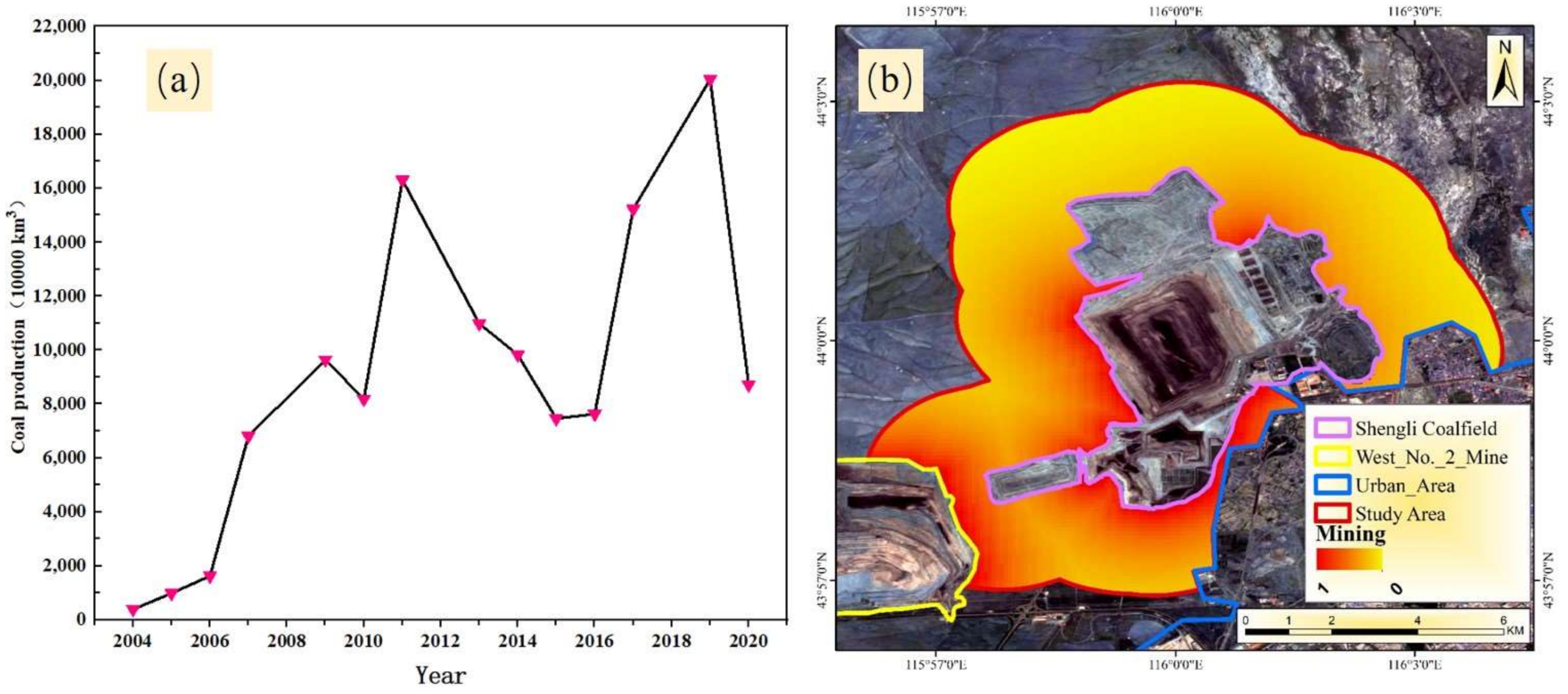
3.1. Study Area
3.2. Fractional Vegetation Coverage
3.3. Driving Factors
3.4. Model Building
4. Results
4.1. Modeling Results and Accuracy
4.2. FVC Spatial Changes and Quantitative Results of Driving Factors
4.3. Contribution Analysis of the Mining Factor
5. Discussion
6. Conclusions
- (1)
- For the 50 models, the average RMSE was 0.052 and the average MRE was 0.007. The GWDF-ANN model is suitable for quantifying FVC changes in mining areas.
- (2)
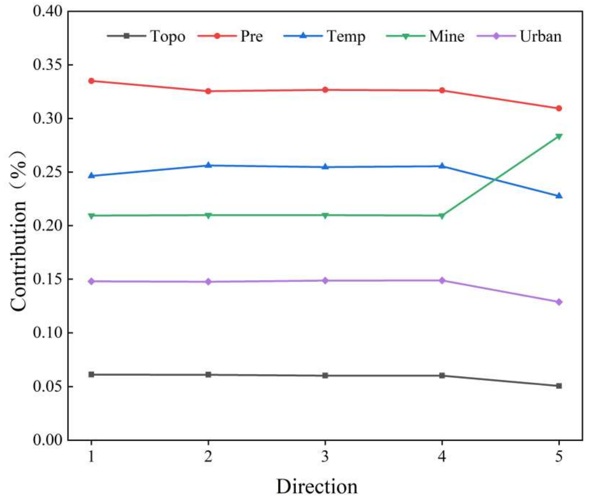
- Precipitation and temperature were the main driving factors for FVC change. The contributions were 32.45% for precipitation, 24.80% for temperature, 22.44% for mining, 14.44% for urban expansion, and 5.87% for topography.
- (3)
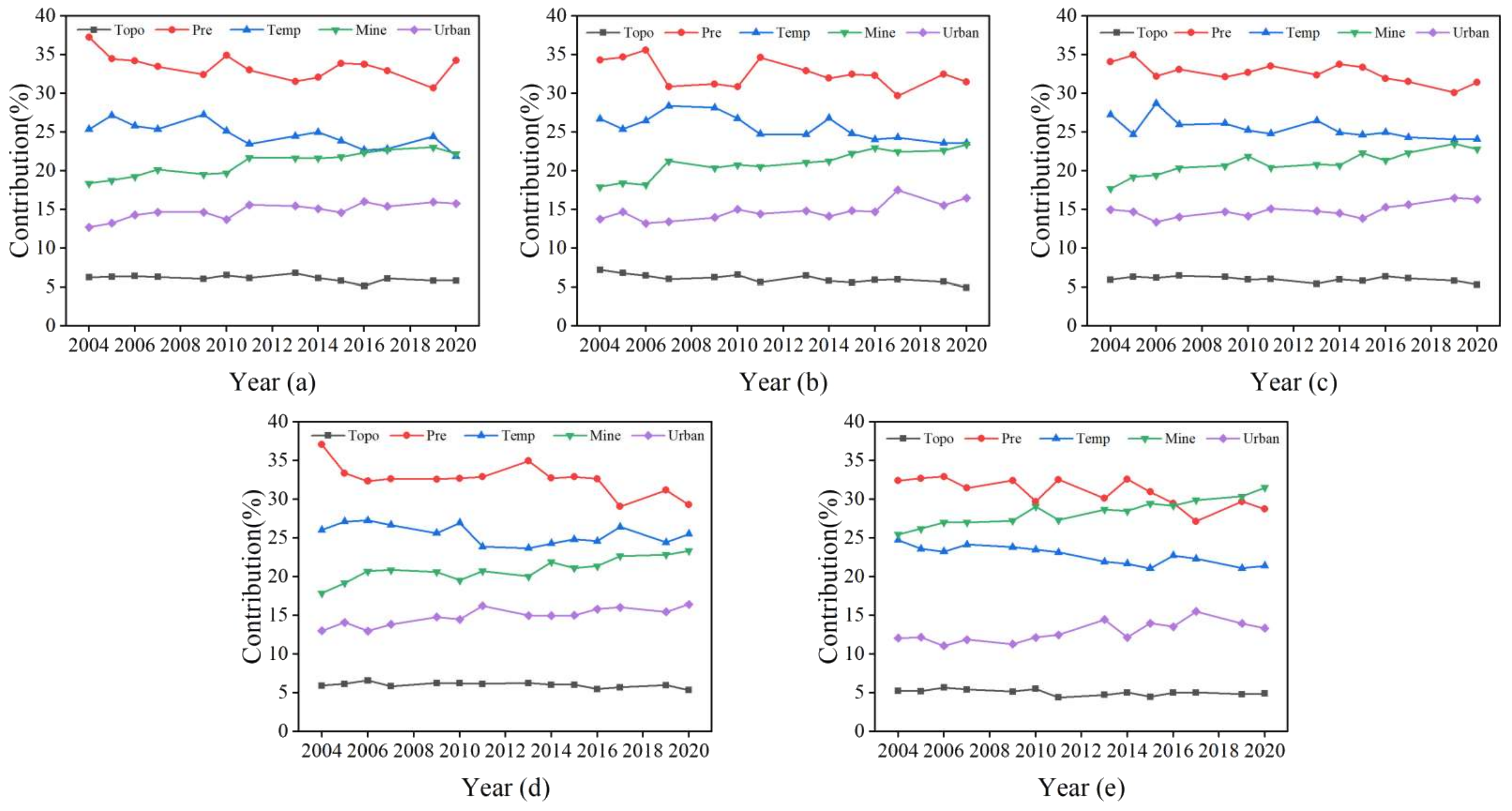
- The contributions of precipitation and temperature on vegetation cover exhibited downward trends, while mining and urban expansion showed positive trajectories. For topography, its contribution remains generally unchanged.
- (4)
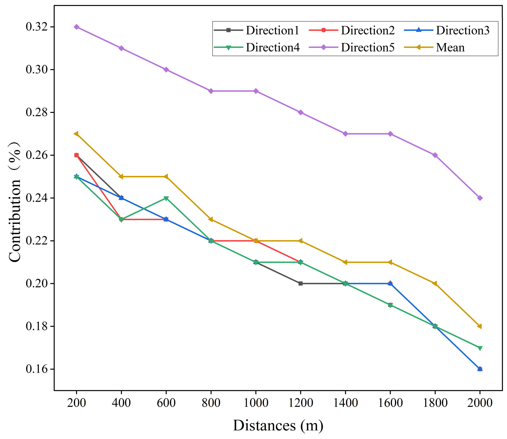
- The contribution of mining showed apparent distance attenuation. At 200 m away, the contribution of mining was 26.69%; at 2000 m away, the value drops to 17.8%.
- (5)
- Mining has a cumulative effect on vegetation coverage both interannually and spatially.
Author Contributions
Funding
Institutional Review Board Statement
Informed Consent Statement
Data Availability Statement
Acknowledgments
Conflicts of Interest
References
- Bai, X.; Ding, H.; Lian, J.; Ma, D.; Yang, X.; Sun, N.; Xue, W.; Chang, Y. Coal production in China: Past, present, and future projections. Int. Geol. Rev. 2017, 60, 535–547. [Google Scholar] [CrossRef]
- Wang, Y.J. Rearch Progress and Prospect on Ecological Disturbance Monitoring in Mining Area. Acta Geod. Cartogr. Sin. 2017, 45, 1705–1716. [Google Scholar]
- Liu, S.J.; Wang, Z.; Mao, Y.C.; Xu, B.S.; Wu, L.X. Multi-source Remote Sensing Technology for Monitoring Safety and Environment in Mine. Geomat. Spat. Inf. Technol. 2015, 38, 98–100. [Google Scholar]
- Wu, Z.; Lei, S.; Lu, Q.; Bian, Z. Impacts of Large-Scale Open-Pit Coal Base on the Landscape Ecological Health of Semi-Arid Grasslands. Remote Sens. 2019, 11, 1820. [Google Scholar] [CrossRef] [Green Version]
- Qian, T.; Bagan, H.; Kinoshita, T.; Yamagata, Y. Spatial–Temporal Analyses of Surface Coal Mining Dominated Land Degradation in Holingol, Inner Mongolia. IEEE J. Sel. Top. Appl. Earth Obs. Remote Sens. 2014, 7, 1675–1687. [Google Scholar] [CrossRef]
- Parmesan, C.; Yohe, G. A globally coherent fingerprint of climate change impacts across natural systems. Nature. 2003, 421, 37–42. [Google Scholar] [CrossRef] [PubMed]
- Chen, L.F.; Zhang, H.; Zhang, X.Y.; Liu, P.H.; Zhang, W.C.; Ma, X.Y. Vegetation changes in coal mining areas: Naturally or anthropogenically Driven? Catena 2022, 208, 105712. [Google Scholar] [CrossRef]
- Hao, L.; Sun, G.; Liu, Y.; Gao, Z.; He, J.; Shi, T.; Wu, B. Effects of precipitation on grassland ecosystem restoration under grazing exclusion in Inner Mongolia, China. Landsc. Ecol. 2014, 29, 1657–1673. [Google Scholar] [CrossRef]
- Chuai, X.W.; Huang, X.J.; Wang, W.J.; Bao, G. NDVI, temperature and precipitation changes and their relationships with different vegetation types during 1998–2007 in Inner Mongolia, China. Int. J. Climatol. 2013, 33, 1696–1706. [Google Scholar] [CrossRef]
- Pang, J.; Du, Z.Q.; Zhang, X.Y. Understanding of the relationship between vegetation change and physical geographic factors based on Geographical Detector. In Proceedings of the International Conference on Intelligent Earth Observing and Applications (IEOAs), Guilin, China, 9 December 2015; pp. 23–24. [Google Scholar]
- Mu, S.J.; Chen, Y.Z.; Li, J.L.; Ju, W.M.; Odeh, I.O.A.; Zou, X.L. Grassland dynamics in response to climate change and human activities in Inner Mongolia, China between 1985 and 2009. Rangel. J. 2013, 35, 315–329. [Google Scholar] [CrossRef]
- Li, J.; Deng, X.J.; Yang, Z.; Liu, Q.L.; Wang, Y.; Cui, L.Y. A Method of Extracting Mining Disturbance in Arid Grassland Based on Time Series Multispectral Images. Spectrosc. Spectr. Anal. 2019, 39, 3788–37893. [Google Scholar]
- Wang, K.W.; Li, J.; Wang, R.G.; Fu, X. Spatial heterogeneity monitoring of temporal variation of vegetation coverage in Shengli mining area. Bull. Surv. Mapp. 2020, 11, 1–6. [Google Scholar] [CrossRef]
- Li, J.; Yan, X.G.; Yan, X.X.; Guo, W.; Wang, K.W.; Qiao, J. Temporal and spatial variation characteristic of vegetation coverage in the Yellow River Basin based on GEE cloud platform. J. China Coal Soc. 2021, 46, 1439–1450. [Google Scholar] [CrossRef]
- Li, X.H.; Lei, S.G.; Cheng, W.; Liu, F.; Wang, W.Z. Spatio-temporal dynamics of vegetation in Jungar Banner of China during 2000–2017. J. Arid. Land 2019, 11, 837–854. [Google Scholar] [CrossRef] [Green Version]
- Yang, Y.; Erskine, P.D.; Lechner, A.M.; Mulligan, D.; Zhang, S.; Wang, Z. Detecting the dynamics of vegetation disturbance and recovery in surface mining area via Landsat imagery and LandTrendr algorithm. J. Clean. Prod. 2018, 178, 353–362. [Google Scholar] [CrossRef]
- Yan, X.; Li, J.; Shao, Y.; Hu, Z.; Yang, Z.; Yin, S.; Cui, L. Driving forces of grassland vegetation changes in Chen Barag Banner, Inner Mongolia. GISci. Remote Sens. 2020, 57, 753–769. [Google Scholar] [CrossRef]
- Fu, X.; Ma, M.; Jiang, P.; Quan, Y. Spatiotemporal vegetation dynamics and their influence factors at a large coal-fired power plant in Xilinhot, Inner Mongolia. Int. J. Sustain. Dev. World Ecol. 2016, 24, 433–438. [Google Scholar] [CrossRef]
- Stewart Fotheringham, A.; Charlton, M.; Brunsdon, C. The geography of parameter space: An investigation of spatial non-stationarity. Int. J. Geogr. Inf. Syst. 1996, 10, 605–627. [Google Scholar] [CrossRef]
- Bitter, C.; Mulligan, G.F.; Dall’erba, S. Incorporating spatial variation in housing attribute prices: A comparison of geographically weighted regression and the spatial expansion method. J. Geogr. Syst. 2006, 9, 7–27. [Google Scholar] [CrossRef] [Green Version]
- Huang, B.; Wu, B.; Barry, M. Geographically and temporally weighted regression for modeling spatio-temporal variation in house prices. Int. J. Geogr. Inf. Sci. 2010, 24, 383–401. [Google Scholar] [CrossRef]
- Yu, W.; Zang, S.; Wu, C.; Liu, W.; Na, X. Analyzing and modeling land use land cover change (LUCC) in the Daqing City, China. Appl. Geogr. 2011, 31, 600–608. [Google Scholar] [CrossRef]
- Hagenauer, J.; Helbich, M. Local modelling of land consumption in Germany with RegioClust. Int. J. Appl. Earth Obs. Geoinf. 2018, 65, 46–56. [Google Scholar] [CrossRef]
- Nelson, A.; Oberthür, T.; Cook, S. Multi-scale correlations between topography and vegetation in a hillside catchment of Honduras. Int. J. Geogr. Inf. Sci. 2007, 21, 145–174. [Google Scholar] [CrossRef]
- Waller, L.A.; Zhu, L.; Gotway, C.A.; Gorman, D.M.; Gruenewald, P.J. Quantifying geographic variations in associations between alcohol distribution and violence: A comparison of geographically weighted regression and spatially varying coefficient models. Stoch. Environ. Res. Risk Assess. 2007, 21, 573–588. [Google Scholar] [CrossRef]
- Wang, L.; Lee, G.; Williams, I. The Spatial and Social Patterning of Property and Violent Crime in Toronto Neighbourhoods: A Spatial-Quantitative Approach. Isprs Int. J. Geo-Inf. 2019, 8, 51. [Google Scholar] [CrossRef] [Green Version]
- Hagenauer, J.; Helbich, M. A geographically weighted artificial neural network. Int. J. Geogr. Inf. Sci. 2021, 36, 215–235. [Google Scholar] [CrossRef]
- Feng, L.; Wang, Y.; Zhang, Z.; Du, Q. Geographically and temporally weighted neural network for winter wheat yield prediction. Remote Sens. Environ. 2021, 262, 112514. [Google Scholar] [CrossRef]
- Masrur, A.; Yu, M.; Mitra, P.; Peuquet, D.; Taylor, A. Interpretable Machine Learning for Analysing Heterogeneous Drivers of Geographic Events in Space-Time. Available online: https://pennstate.pure.elsevier.com/en/publications/interpretable-machine-learning-for-analysing-heterogeneous-driver (accessed on 15 September 2021).
- Gitelson, A.A.; Kaufman, Y.J.; Stark, R.; Rundquist, D. Novel algorithms for remote estimation of vegetation fraction. Remote Sens. Environ. 2002, 80, 76–87. [Google Scholar] [CrossRef] [Green Version]
- Purevdorj, T.S.; Tateishi, R.; Ishiyama, T.; Honda, Y. Relationships between percent vegetation cover and vegetation indices. Int. J. Remote Sens. 2010, 19, 3519–3535. [Google Scholar] [CrossRef]
- Zhang, C.Y.; Li, J.; Lei, S.G.; Yang, J.Z.; Yang, N. Progress and prospect of the Quantitative Remote Sensing for Monitoring the Eco-Environment in Mining Areas. Available online: http://kns.cnki.net/kcms/detail/34.1055.TD.20210915.1042.002.html (accessed on 4 August 2021).
- Bao, Y.H.; Bao, S.Y.; Shan, Y. Analysis on Temporal and Spatial Changes of Landscape Pattern in Dalinor Lake Wetland. In Proceedings of the 3rd International Conference on Environmental Science and Information Application Technology (ESIAT), Xi’an, China, 20–21 August 2011; pp. 2367–2375. [Google Scholar]
- Li, F.; Lawrence, D.M. Role of Fire in the Global Land Water Budget during the Twentieth Century due to Changing Ecosystems. J. Clim. 2017, 30, 1893–1908. [Google Scholar] [CrossRef]
- Lecun, Y.; Bengio, Y.; Hinton, G. Deep learning. Nature 2015, 521, 436–444. [Google Scholar] [CrossRef] [PubMed]
- Rojas, R. Neural Networks: A Systematic Introduction; Springer Science & Business Media: Berlin/Heidelberg, Germany, 2013. [Google Scholar]
- Rumelhart, D.E.; Hinton, G.E.; Williams, R.J.J.N. Learning representations by back-propagating errors. Nature 1986, 323, 533–536. [Google Scholar] [CrossRef]
- Nesterov, Y. A Method of Solving a Convex Programming Problem with Convergence Rate. Dokl. Chem. 1983, 27, 372–376. [Google Scholar]
- Sutskever, I.; Martens, J.; Dahl, G.; Hinton, G. On the importance of initialization and momentum in deep learning. In Proceedings of the International Conference on Machine Learning, Atlanta, GA, USA, 16 June 2013; pp. 1139–1147. [Google Scholar]
- Flood, N. Continuity of Reflectance Data between Landsat-7 ETM+ and Landsat-8 OLI, for Both Top-of-Atmosphere and Surface Reflectance: A Study in the Australian Landscape. Remote Sens. 2014, 6, 7952–7970. [Google Scholar] [CrossRef] [Green Version]
- Li, P.; Jiang, L.; Feng, Z. Cross-Comparison of Vegetation Indices Derived from Landsat-7 Enhanced Thematic Mapper Plus (ETM+) and Landsat-8 Operational Land Imager (OLI) Sensors. Remote Sens. 2013, 6, 310–329. [Google Scholar] [CrossRef] [Green Version]
- She, X.; Zhang, L.; Cen, Y.; Wu, T.; Huang, C.; Baig, M. Comparison of the Continuity of Vegetation Indices Derived from Landsat 8 OLI and Landsat 7 ETM+ Data among Different Vegetation Types. Remote Sens. 2015, 7, 13485–13506. [Google Scholar] [CrossRef] [Green Version]
- Bai, S.Y.; Wang, L.; Shi, J.Q. Time lag effect of NDVI response to climatic change in Yangtze River basin. Chin. J. Agrometeorol. 2012, 33, 579–586. [Google Scholar]
- Wang, J.B.; Yang, X.L.; Zhang, Y.H.; Wang, X.W. Correlation Between NDVI and Meteorological Factors in Zhangye. Chin. Agric. Sci. Bull. 2019, 35, 85–90. [Google Scholar]
- Liu, Y.L.; Guo, L.; Jiang, Q.H.; Zhang, H.T.; Chen, Y.Y. Comparing geospatial techniques to predict SOC stocks. Soil Tillage Res. 2015, 148, 46–58. [Google Scholar] [CrossRef]
- Arora, A.; Pandey, M.; Mishra, V.N.; Kumar, R.; Rai, P.K.; Costache, R.; Punia, M.; Di, L. Comparative evaluation of geospatial scenario-based land change simulation models using landscape metrics. Ecol. Indic. 2021, 128, 107810. [Google Scholar] [CrossRef]
- Chen, Z.F.; Wang, W.G.; Fu, J.Y. Vegetation response to precipitation anomalies under different climatic and biogeographical conditions in China. Sci. Rep. 2020, 10, 1–16. [Google Scholar] [CrossRef] [Green Version]
- Shen, X.J.; Liu, B.H.; Li, G.D.; Yu, P.J.; Zhou, D.W. Impacts of grassland types and vegetation cover changes on surface air temperature in the regions of temperate grassland of China. Theor. Appl. Climatol. 2016, 126, 141–150. [Google Scholar] [CrossRef]
- Liu, Y.; Shu, H.; Li, Y. Correlation Analysis of Spatio-temporal NDVI, Air Temperature, Precipitation, and Ground Temperature in the Bayinbuluk Grassland. In Proceedings of the IEEE International Geoscience and Remote Sensing Symposium (IGARSS), Denver, CO, USA, 1 July 2006; p. 3368. [Google Scholar]
- Zhang, Y.; Liang, W.; Liao, Z.; Han, Z.; Xu, X.; Jiao, R.; Liu, H. Effects of climate change on lake area and vegetation cover over the past 55 years in Northeast Inner Mongolia grassland, China. Theor. Appl. Climatol. 2019, 138, 13–25. [Google Scholar] [CrossRef]
- Fang, A.; Bao, M.; Chen, W.; Dong, J. Assessment of Surface Ecological Quality of Grassland Mining Area and Identification of Its Impact Range. Nat. Resour. Res. 2021, 30, 3819–3837. [Google Scholar] [CrossRef]
- Hui, J.; Bai, Z.; Ye, B.; Wang, Z. Remote Sensing Monitoring and Evaluation of Vegetation Restoration in Grassland Mining Areas—A Case Study of the Shengli Mining Area in Xilinhot City, China. Land 2021, 10, 743. [Google Scholar] [CrossRef]
- Ohana-Levi, N.; Paz-Kagan, T.; Panov, N.; Peeters, A.; Tsoar, A.; Karnieli, A. Time series analysis of vegetation-cover response to environmental factors and residential development in a dryland region. Gisci. Remote Sens. 2019, 56, 362–387. [Google Scholar] [CrossRef] [Green Version]
- Song, X.P.; Hansen, M.C.; Stehman, S.V.; Potapov, P.V.; Tyukavina, A.; Vermote, E.F.; Townshend, J.R. Author Correction: Global land change from 1982 to 2016. Nature 2018, 563, E26. [Google Scholar] [CrossRef] [Green Version]
- Wang, Z.; Deng, X.; Song, W.; Li, Z.; Chen, J. What is the main cause of grassland degradation? A case study of grassland ecosystem service in the middle-south Inner Mongolia. Catena 2017, 150, 100–107. [Google Scholar] [CrossRef]
- Xu, G.; Zhang, J.; Li, P.; Li, Z.; Lu, K.; Wang, X.; Wang, F.; Cheng, Y.; Wang, B. Vegetation restoration projects and their influence on runoff and sediment in China. Ecol. Indic. 2018, 95, 233–241. [Google Scholar] [CrossRef]
- Jiang, G.; Han, X.; Wu, J. Restoration and management of the Inner Mongolia grassland require a sustainable strategy. AMBIO A J. Hum. Environ. 2006, 35, 269–270. [Google Scholar] [CrossRef]


| Sensor | Year | Path/Row | Date | Number | |||||
|---|---|---|---|---|---|---|---|---|---|
| Landsat 8 OLI | 2020 | 124/29 | 9 July | 25 July | 10 August | 26 August | 11 September | 27 September | 16 |
| 124/30 | 9 July | 25 July | 10 August | 26 August | 11 September | 27 September | |||
| 125/29 | 16 July | 1 August | 2 September | 18 September | |||||
| 2019 | 124/29 | 7 July | 23 July | 8 August | 24 August | 9 September | 25 September | 16 | |
| 124/30 | 7 July | 23 July | 8 August | 24 August | 9 September | 25 September | |||
| 125/29 | 14 July | 31 July | 31 August | 16 September | |||||
| 2017 | 124/29 | 1 July | 17 July | 18 August | 3 September | 19 September | 16 | ||
| 124/30 | 1 July | 17 July | 18 August | 3 September | 19 September | ||||
| 125/29 | 8 July | 24 July | 9 August | 25 August | 10 September | 26 September | |||
| 2016 | 124/29 | 14 July | 30 July | 21 August | 16 September | 14 | |||
| 124/30 | 14 July | 30 July | 21 August | 16 September | |||||
| 125/29 | 5 July | 21 July | 6 August | 22 August | 7 September | 23 September | |||
| 2015 | 124/29 | 12 July | 28 July | 13 August | 29 August | 14 September | 30 September | 18 | |
| 124/30 | 12 July | 28 July | 13 August | 29 August | 14 September | 30 September | |||
| 125/29 | 3 July | 19 July | 4 August | 20 August | 5 September | 21 September | |||
| 2014 | 124/29 | 9 July | 25 July | 10 August | 26 August | 11 September | 27 September | 16 | |
| 124/30 | 9 July | 25 July | 10 August | 26 August | 11 September | 27 September | |||
| 125/29 | 16 July | 1 August | 2 September | 18 September | |||||
| 2013 | 124/29 | 6 July | 22 July | 7 August | 23 August | 8 September | 24 September | 16 | |
| 124/30 | 6 July | 22 July | 7 August | 23 August | 8 September | 24 September | |||
| 125/29 | 13 July | 30 July | 30 August | 15 September | |||||
| Landsat 5 TM | 2011 | 124/29 | 1 July | 17 July | 18 August | 3 September | 19 September | 16 | |
| 124/30 | 1 July | 17 July | 18 August | 3 September | 19 September | ||||
| 125/29 | 8 July | 24 July | 9 August | 25 August | 10 September | 26 September | |||
| 2010 | 124/29 | 14 July | 30 July | 21 August | 16 September | 14 | |||
| 124/30 | 14 July | 30 July | 21 August | 16 September | |||||
| 125/29 | 5 July | 21 July | 6 August | 22 August | 7 September | 23 September | |||
| 2009 | 124/29 | 11 July | 27 July | 12 August | 28 August | 13 September | 29 September | 18 | |
| 124/30 | 11 July | 27 July | 12 August | 28 August | 13 September | 29 September | |||
| 125/29 | 2 July | 18 July | 3 August | 19 August | 4 September | 20 September | |||
| 2007 | 124/29 | 6 July | 22 July | 7 August | 23 August | 8 September | 24 September | 16 | |
| 124/30 | 6 July | 22 July | 7 August | 23 August | 8 September | 24 September | |||
| 125/29 | 13 July | 30 July | 30 August | 15 September | |||||
| 2006 | 124/29 | 3 July | 29 July | 4 August | 20 August | 5 September | 21 September | 17 | |
| 124/30 | 3 July | 29 July | 4 August | 20 August | 5 September | 21 September | |||
| 125/29 | 10 July | 27 July | 27 August | 12 September | 28 September | ||||
| 2005 | 124/29 | 16 July | 17 August | 2 September | 18 September | 14 | |||
| 124/30 | 16 July | 17 August | 2 September | 18 September | |||||
| 125/29 | 7 July | 23 August | 7 August | 24 August | 9 September | 25 September | |||
| 2004 | 124/29 | 13 July | 29 July | 14 August | 30 August | 15 September | 16 | ||
| 124/30 | 13 July | 29 July | 14 August | 30 August | 15 September | ||||
| 125/29 | 4 July | 20 July | 5 August | 21 August | 6 September | 22 September | |||
| Model 1 | Model 2 | Model 3 | Model 4 | Model 5 | Model 6 | Model 7 | Model 8 | Model 9 | Model 10 | |
|---|---|---|---|---|---|---|---|---|---|---|
| RMSE | 0.0577 | 0.0567 | 0.0654 | 0.0642 | 0.0506 | 0.0493 | 0.0548 | 0.0554 | 0.0853 | 0.1117 |
| MRE | 0.0064 | 0.0084 | 0.0061 | 0.0035 | 0.0019 | 0.0014 | 0.0040 | 0.0006 | 0.0023 | 0.0162 |
| Model 11 | Model 12 | Model 13 | Model 14 | Model 15 | Model 16 | Model 17 | Model 18 | Model 19 | Model 20 | |
| RMSE | 0.0537 | 0.0621 | 0.0190 | 0.0173 | 0.0262 | 0.0066 | 0.0334 | 0.0148 | 0.0935 | 0.0141 |
| MRE | 0.0095 | 0.0056 | 0.0076 | 0.0032 | 0.0085 | 0.0044 | 0.0061 | 0.0078 | 0.0080 | 0.0015 |
| Model 21 | Model 22 | Model 23 | Model 24 | Model 25 | Model 26 | Model 27 | Model 28 | Model 29 | Model 30 | |
| RMSE | 0.0468 | 0.0930 | 0.0139 | 0.0954 | 0.0142 | 0.0630 | 0.0597 | 0.0709 | 0.0805 | 0.0963 |
| MRE | 0.0218 | 0.0042 | 0.0058 | 0.0025 | 0.0076 | 0.0083 | 0.0039 | 0.0087 | 0.0086 | 0.0020 |
| Model 31 | Model 32 | Model 33 | Model 34 | Model 35 | Model 36 | Model 37 | Model 38 | Model 39 | Model 40 | |
| RMSE | 0.0706 | 0.0688 | 0.0178 | 0.0230 | 0.0167 | 0.0522 | 0.0256 | 0.0352 | 0.0931 | 0.0888 |
| MRE | 0.0038 | 0.0068 | 0.0042 | 0.0073 | 0.0043 | 0.0096 | 0.0078 | 0.0085 | 0.0057 | 0.0072 |
| Model 41 | Model 42 | Model 43 | Model 44 | Model 45 | Model 46 | Model 47 | Model 48 | Model 49 | Model 50 | |
| RMSE | 0.0494 | 0.0598 | 0.0671 | 0.0223 | 0.0246 | 0.0660 | 0.0399 | 0.0883 | 0.0143 | 0.0569 |
| MRE | 0.0074 | 0.0078 | 0.0034 | 0.0120 | 0.0093 | 0.0234 | 0.0056 | 0.0126 | 0.0056 | 0.0130 |
Publisher’s Note: MDPI stays neutral with regard to jurisdictional claims in published maps and institutional affiliations. |
© 2022 by the authors. Licensee MDPI, Basel, Switzerland. This article is an open access article distributed under the terms and conditions of the Creative Commons Attribution (CC BY) license (https://creativecommons.org/licenses/by/4.0/).
Share and Cite
Li, J.; Qin, T.; Zhang, C.; Zheng, H.; Guo, J.; Xie, H.; Zhang, C.; Zhang, Y. A New Method for Quantitative Analysis of Driving Factors for Vegetation Coverage Change in Mining Areas: GWDF-ANN. Remote Sens. 2022, 14, 1579. https://doi.org/10.3390/rs14071579
Li J, Qin T, Zhang C, Zheng H, Guo J, Xie H, Zhang C, Zhang Y. A New Method for Quantitative Analysis of Driving Factors for Vegetation Coverage Change in Mining Areas: GWDF-ANN. Remote Sensing. 2022; 14(7):1579. https://doi.org/10.3390/rs14071579
Chicago/Turabian StyleLi, Jun, Tingting Qin, Chengye Zhang, Huiyu Zheng, Junting Guo, Huizhen Xie, Caiyue Zhang, and Yicong Zhang. 2022. "A New Method for Quantitative Analysis of Driving Factors for Vegetation Coverage Change in Mining Areas: GWDF-ANN" Remote Sensing 14, no. 7: 1579. https://doi.org/10.3390/rs14071579