Article

Quantifying Post-Fire Changes in the Aboveground Biomass of an Amazonian Forest Based on Field and Remote Sensing Data

by
Aline Pontes-Lopes
1,*,
Ricardo Dalagnol
1,2,3,
Andeise Cerqueira Dutra
1,
Camila Valéria de Jesus Silva
4,5,
Paulo Maurício Lima de Alencastro Graça
6 and
Luiz Eduardo de Oliveira e Cruz de Aragão
1,7
1
Earth Observation and Geoinformatics Division, National Institute for Space Research (INPE), São José dos Campos 12227-010, Brazil
2
NASA-Jet Propulsion Laboratory, California Institute of Technology, Pasadena, CA 91109, USA
3
Institute of the Environment and Sustainability, University of California, Los Angeles, CA 90095, USA
4
Lancaster Environment Centre, Lancaster University, Lancaster LA1 4YQ, UK
5
Amazon Environmental Research Institute (IPAM), Brasília 71503-505, Brazil
6
Environmental Dynamics Coordination, National Institute for Research in Amazonia (INPA), Manaus 69067-375, Brazil
7
College of Life and Environmental Sciences, University of Exeter, Exeter EX4 4RJ, UK
*
Author to whom correspondence should be addressed.
Remote Sens. 2022, 14(7), 1545; https://doi.org/10.3390/rs14071545
Submission received: 8 February 2022 / Revised: 11 March 2022 / Accepted: 16 March 2022 / Published: 23 March 2022

Abstract

:
Fire is a major forest degradation component in the Amazon forests. Therefore, it is important to improve our understanding of how the post-fire canopy structure changes cascade through the spectral signals registered by medium-resolution satellite sensors over time. We contrasted accumulated yearly temporal changes in forest aboveground biomass (AGB), measured in permanent plots, and in traditional spectral indices derived from Landsat-8 images. We tested if the spectral indices can improve Random Forest (RF) models of post-fire AGB losses based on pre-fire AGB, proxied by AGB data from immediately after a fire. The delta normalized burned ratio, non-photosynthetic vegetation, and green vegetation (ΔNBR, ΔNPV, and ΔGV, respectively), relative to pre-fire data, were good proxies of canopy damage through tree mortality, even though small and medium trees were the most affected tree size. Among all tested predictors, pre-fire AGB had the highest RF model importance to predicting AGB within one year after fire. However, spectral indices significantly improved AGB loss estimates by 24% and model accuracy by 16% within two years after a fire, with ΔGV as the most important predictor, followed by ΔNBR and ΔNPV. Up to two years after a fire, this study indicates the potential of structural and spectral-based spatial data for integrating complex post-fire ecological processes and improving carbon emission estimates by forest fires in the Amazon.

1. Introduction

The Amazon is facing a scenario of increasing forest degradation [1,2]. Moreover, in the Brazilian Amazon, this process is potentially causing greater carbon losses than those from deforestation [3]. Forest degradation is here defined as a human-induced process of forest impoverishment (mainly in terms of structural complexity and biomass stock), resulting from logging, fire, and edge effects associated with human activities. The fire contribution to this process may further increase with climate change and deforestation [4,5], representing a major threat to the Amazonian forests in Brazil, especially with the planned opening/repaving of regional roads without additional environmental regulations [6,7]. It is estimated that forest fire degradation led to gross CO2 emissions of 454 ± 496 Tg year−1 during 2003–2015, representing ~31% of CO2 emissions from deforestation in years of regular rainfall and reaching over 50% of deforestation emissions during extremely dry years (e.g., 2010 and 2015) [8]. However, these estimates are highly uncertain and must be improved to correctly quantify their contributions to the global carbon cycle and to national greenhouse gas inventories in tropical countries [9,10].
Forest fires in the Amazon—not related to deforestation activities—are often of low intensity and spread [11,12], being restricted to the floor if affecting standing dense forests [11,12,13,14,15]. This low intensity causes markedly size- and time-dependent tree mortality [16,17,18], immediately killing most saplings (e.g., up to 10 cm of diameter at breast height, DBH) [19], markedly affecting small trees (10–30 cm of DBH) up to three years after a fire [14,20], and potentially leading to delayed mortality of large trees (DBH > 40 cm) up to about eight years after a fire [18,20]. However, both fire intensity and post-fire impacts present high intra- and inter-site spatial heterogeneity [14,16]. For example, fire-mediated tree mortality can represent 9 to 50% of the forest aboveground biomass (AGB) up to 3 years after a fire event [14,16], being a function of interrelated external and internal factors. External factors are regular regional climate and extreme climatic events, regulating drought frequency and intensity [21,22,23,24]. Internal factors determine forest microclimatic characteristics, fuel availability, and fire sensitivity/resistance, such as forest structure, e.g., canopy height and tree size distribution [12,25]; terrain and soil characteristics, e.g., flooding forest types and white-sand soils [26,27]; species composition, e.g., the presence of sensitive/protective plant traits [28,29,30]. As well as tree size (e.g., DBH), wood density is an important plant trait that affects post-fire mortality, with the smaller tree sizes and lower wood-density trees having a greater probability to die in the earlier post-fire years [14,28,29].
To develop maps of estimated fire effects and carbon emissions, it is necessary to find emergent properties, estimated from satellite data, that can integrate these several complex fire-associated factors to scale-up field measurements to broader scales. An integrative variable should be ideally of easy measurement and highly correlated to other variables of more complex measurement. For example, pre-fire AGB is considered an important integrative variable [25] since it is related to tree size distribution, wood densities, and microclimate moisture, which affects forest flammability [12,17]. Previous works have therefore used aboveground carbon-density maps [31,32] as the pre-fire AGB to predict post-fire AGB across broad areas in the Amazon based on a factor of AGB loss [13,25,33]. However, these factors were developed only for the first year after fire and later AGB losses (e.g., up to 3 years after a fire) are more difficult to model. Other potential integrative variables, associated with forest dynamics and perhaps mainly tree mortality, are temporal changes (∆) in remotely sensed spectral indices, such as the normalized burn ratio (NBR) [34,35,36] and subpixel fractions, e.g., non-photosynthetic vegetation (NPV), photosynthetic or green vegetation (GV), and shade [15,37,38]. The ∆NBR was developed to define classes of burn severity in temperate areas [39,40] but has also been applied to tropical areas [36,41,42]. The ∆NPV has been used to estimate the fraction and the absolute number of dead trees in regular canopy gaps and forest areas affected by convective storms (blowdowns) in the Amazon [38,43]. Nevertheless, to the best of our knowledge, there are no previous works so far that have used changes in spectral indices to estimate changes in AGB for Amazonian forests.
In this context, we investigated the potential of integrating temporal changes in these traditional remote sensing spectral indices (NBR and NPV-GV-Shade fractions) derived from Landsat satellite images to improve the aforementioned AGB loss-factor method for predicting post-fire AGB losses. For this, we used a forest AGB dataset from an earlier field study [14] based on yearly measurements of fire-affected permanent forest plots, installed immediately after an El Niño understory fire (~2 months) in a dense non-flooded forest in the Central Amazon. The mentioned field study has shown that this area was affected by an understory fire of low intensity and irregular spread, leading to 27.3% of stem mortality and 12.8% of AGB loss (DBH ≥ 10 cm) up to three years after the fire, concentrated in small and medium trees. This post-fire dataset [14] was used to investigate the following three groups of questions that support our prediction method:
Q1. Does the pre-fire AGB define the post-fire impact on forest AGB?
Q2. How is the response of spectral indices to these post-fire changes?
Q3. Does the addition of temporal changes in spectral indices to pre-fire AGB improve the regression models’ capability to predict post-fire AGB losses? Which predictive variables are most important?

2. Materials and Methods

2.1. Study Area

Our study area is located in the northern Purus-Madeira interfluve, a dense moist forest region [44], specifically at 3°31′ South and 59°15′ West, about ~90 km southeast of Manaus (Brazil), in the central Brazilian Amazon (Figure 1a). This is a lowland region, i.e., an extensive flat surface of medium to low soil drainage, dissected by broad seasonal floodplains, covered by dense non-flooded (terra firme) and seasonally flooded forests [45]. According to the Climate Hazards group Infrared Precipitation with Stations (CHIRPS) rainfall product [46], annual rainfall varies from 2000 to 2400 mm with the dry season typically ranging from July to September (3 months year−1). According to data from the MCD64A1 Moderate Resolution Imaging Spectroradiometer (MODIS) burned area product [47], understory fires affected ~230 km2 of forests, i.e., ~23 thousand soccer fields of forests, in the northern interfluve during the extreme 2015 El Niño drought—affecting even old-growth high-biomass forests [14]. Large forest fires in this moist forest region are typically restricted to extreme droughts [14,26]. Further descriptions of the study area can be found in [14].

2.2. Data

2.2.1. Field Dataset

Twelve permanent forest inventory plots were installed in burned dense terra firme forests in the study area in December 2015 (Figure 1b), about two months after the El Niño fire event, for the study of [14]. These burned plots were located at least 250 m from forest edges, in areas without signs of recent burns and tree logging. Each plot was censused annually each November until 2018, totaling four censuses and three measurement intervals of one year (Figure 2).
Each plot was a long transect of 250 × 10 m (0.25 ha each), divided into 10 sectors of 25 × 10 m, and 2 sections of 50 × 10 m (the initial and final 50 m of a permanent plot) (Figure 3). Plot corners have been georeferenced with submeter accuracy using real time kinematic global navigation satellite systems (Trimble Zephyr Geodetic 2 RoHS and Spectra Precision SP60).
The forest inventory encompassed all live trees, palms, and lianas with DBH (i.e., 1.3 m of height above ground) greater than or equal to 10 cm. DBH was recorded for each plant in each year, and also their taxonomic information [14,16,17,48]. This dataset was used to calculate AGB for each permanent plot (250 × 10 m) and each section (50 × 10 m) in each year, using different equations for trees, palms, and lianas [49,50,51]. We also split AGB according to two tree size classes: small and medium trees (DBH < 30 cm) and large trees (DBH ≥ 30 cm). We then calculated the absolute and percentage temporal changes (∆) in AGB, relative to the estimates of December 2015 (hereafter called initial AGB), according to the following equations, respectively
AGB Δ y , p = AGB y , p AGB 2015 , p
AGB Δ % y , p = ( AGB y , p AGB 2015 , p ) AGB 2015 , p × 100
where: AGB = aboveground biomass for all measured life forms (trees, palms, and lianas) or for each tree size (small/medium or large trees); y = year of each remeasurement (2016 to 2018); p = each permanent plot (250 × 10 m) or plot section (50 × 10 m). Note that these temporal changes are based on the assumption that the initial forest structure and biomass, measured in December 2015, are similar to the pre-fire conditions. This assumption is supported by the fact that tree mortality following low intensity fires in the Amazon is size and time dependent [16,18], as previously explained. We do not expect that the plant types (smaller and lower wood-density trees) mostly affected in the immediate post-fire months [11,14,28,29] led to significant changes in the AGB in the two intervening months between the fire and the initial field measurement. Furthermore, there were no strong significant differences in the basal area (BA) of dead standing stems (DBH ≥ 10 cm) between burned and unburned plots in the initial census (2015) (Table A1). All field data were processed in R version 4.0.2 [52].

2.2.2. Remote Sensing Dataset

Landsat-8 Operational Land Imager (OLI) surface reflectance (SR) images (30m-grid) [53]—available in the Google Earth Engine (GEE) data catalog (Collection 1, Tier 1) [54]—were used to calculate post-fire changes in spectral indices. We followed the methods of [55] and used the GEE cloud computing platform for selecting Landsat-8 SR images (bands 1–7) with less than 30% of cloud coverage; eliminating cloud and shadow areas based on the OLI Quality Assessment band. In these steps, we processed images from August to September for 2015 to 2018 (Figure 2), except 2016, which also included one image of early October. We then applied a Linear Spectral Mixing Model (LSMM) [56], called spectral unmixing in GEE [57], to model the spectrum of each pixel from the Landsat-8 images as a linear combination of three targets (NPV, GV, and Shade), minimizing the sum of squared errors, as described in general terms by this equation
r i = a ×   NPV i + b × GV i + c × Shade i   + e i
where: r = surface reflectance of the pixel for the i spectral band; NPV, GV, and Shade = spectral reflectance of the reference target (non-photosynthetic vegetation, photosynthetic vegetation, and shade, respectively) (Figure 4); a, b, and c = proportion/fraction values of the reference targets (NPV, GV, and Shade, respectively); e = residual error. This method results in three fraction images (ac), i.e., each image representing the proportion of each target in our study area. Our reference targets (Figure 4) were manually selected near our study area on a Landsat-8 false-color composite image (RGB654) of September 2016, overlapped with a Sentinel-2 Multispectral Instrument (MSI, L1C) image (10m-grid) [58] for more accurate target identification. The NPV reference was therefore selected in a large forest gap opened on a forest edge, showing a lower near-infrared reflectance than the GV reference; the GV reference in a green forest canopy with few intra-canopy shades; the Shade reference in deep water body—a large river in the same Landsat-8 image.
We also used the selected Landsat-8 images to calculate the NBR [34] by applying a simple band math, according to this equation
NBR = ( NIR SWIR ) / ( NIR + SWIR )
where: NIR = surface reflectance in the near-infrared wavelength (OLI band 5); SWIR = surface reflectance in the shortwave infrared wavelength (OLI band 7).
In GEE, we constructed yearly mosaics (n = 4) of each spectral index (NBR, NPV, GV, and Shade) according to their order in the collection for the selected months to exclude remaining cloud pixels in our area of interest, but gave priority to images of the same month (September) in order to avoid seasonal artifacts, e.g., caused by different canopy leaf phenology behavior, sun-sensor illumination angles, and flood levels [36]. Note that the 2015 mosaic is pre-fire and the others (2016–2018) are post-fire mosaics.
We used these mosaics to calculate the absolute temporal changes (∆) in NPV, GV, and Shade relative to the pre-fire mosaics (2015) (Figure 5), following Equation (5). This calculation followed the reverse order for ∆NBR (Equation (6)) in order that recently burned areas presented positive ∆NBR values [36].
Δ Index y , c = Index y , c Index 2015 , c
Δ NBR y , c = NBR 2015 , c NBR y , c
where: y = each post-fire year (2016 to 2018); c = each 30 m pixel. These raster calculations and all following steps were processed in R version 4.0.2 [52]. This approach was an extended assessment [36], using images with about one-year intervals from the reference image (2015) registered immediately before the fire.
We finally disaggregated each ∆Index image (30m-grid) into a 1 m grid, maintaining their original values, and then calculated the average of all 1m-grid ∆Index values within each burned permanent plot section area (plot’s initial and final 50 × 10 m, n = 24) with a 20 m buffer around their boundaries. This is equivalent to calculating mean index values weighted by proportion of each pixel’s overlap with each buffered field plot section (90 × 50 m). As the forest fire impacts on the forest structure presented high spatial variability even within a plot [14], this section-based clip allowed us to include more homogeneous changes in each ∆AGB value, to average fewer Landsat pixels, and to increase the sample size in comparison to clipping with the entire plot. Furthermore, this 20m-buffer was used because the area occupied by the tree crowns can be ~20 m larger than the area inventoried in field. This buffer size is approximately the radius of a large tree crown.
Note that all field- and Landsat-based change metrics consider three increasing temporal intervals since fire: 2015–2016 (1-year interval), 2015–2017 (2-year interval), and 2015–2018 (3-year interval).

2.3. Data Analyses

To test whether the initial AGB defines the post-fire impacts on forest AGB (Q1), we employed linear regression models to assess the relationships between the initial and the post-fire AGB stocks, absolute changes (∆), and percentage changes (∆%), at both plot level and section level in the three analyzed temporal intervals. To investigate the spectral indices’ temporal behavior (Q2), we also employed linear regressions between the temporal change in the spectral indices and the ∆AGB at section level. We removed an outlier plot (n = 1) where a very large tree had fallen causing an extreme outlier in both plot AGB and spectral indices changes, and three sections (n = 3) due to the large tree gap, evident smoke contamination in the 2015 reference images, or a lack of char marks on trees, i.e., unburned sectors within a burned plot. We checked if the used initial AGB data (split in sections) was spatially autocorrelated using the Moran’s I coefficient [59] from the ape R package [60]. We then adjusted a linear regression for each paired relationship, calculated their coefficient of determination (R2) and significance level, using the ggpubr R package [61].
To evaluate the potential of the spectral indices to improve the accuracy of models to predict post-fire AGB (Q3), we adjusted regression models for each temporal interval. For this purpose, we employed Random Forest (RF) regression, which is a machine learning algorithm that can be used for regression problems based on non-normal data [62]. It creates a combination of numerous decision trees at random samples of training datasets to output average predictions based on the ensemble decision. We used two groups of variables: (1) only the initial AGB; (2) the combination of initial AGB and all spectral indices’ changes (∆NBR, ∆NPV, ∆GV, and ∆Shade). We created RF models for each time interval and predictor group to predict the section level absolute AGB loss (n = 16), which corresponds to those sections with negative changes only, i.e., AGB loss. We trained and evaluated the models with a cross-validation approach (CV) of 100 iterations. In each iteration, we randomly subset 70% of the samples to train the models and 30% to evaluate model errors. We trained the models with the bootstrap sampling method, using 500 decision trees and selecting the optimal mtry hyperparameter for the modelling considering the smallest Root Mean Squared Error (RMSE). In all iterations, selected mtry was 2. We then evaluated model performance using the coefficient of determination (CV-R2) and the normalized RMSE (CV-RMSE%), relative to the mean AGB loss of all sample plots. We also evaluated the average absolute importance of each predictor from the full models by computing multiple pairwise comparisons using the Tukey’s Honest Significant Difference tests. Finally, we produced partial dependent plots to evaluate the marginal effects of each variable on predicting AGB loss values. Note that, as the section-level ∆NBR and the ∆NPV are highly correlated (Pearson’s r = ~0.86), we discarded one of them from the full models, keeping that which generated the highest average R2. These analyses were performed with the randomForest, caret, pdp, and multcomp R packages [63,64,65,66,67,68].

3. Results

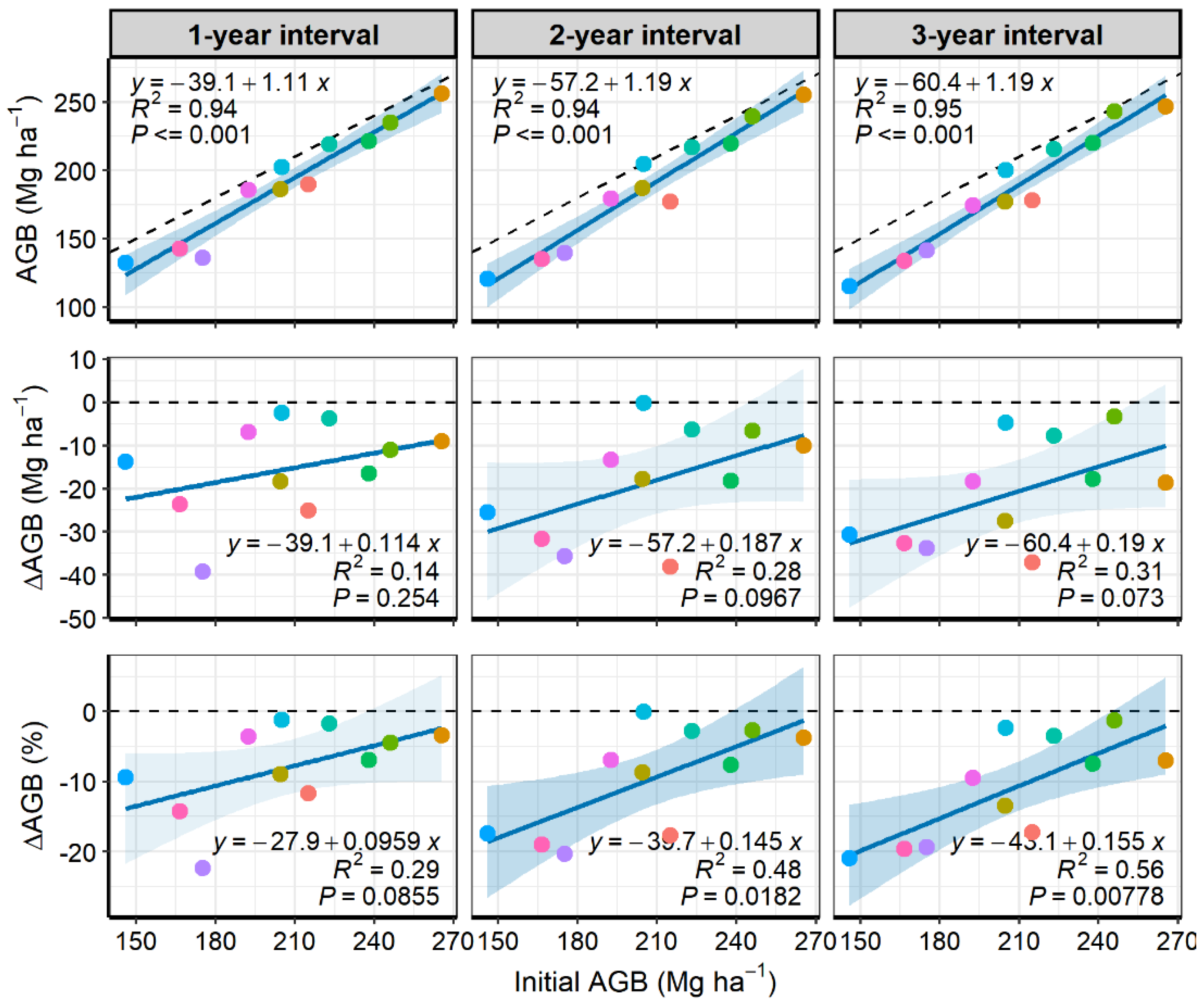
3.1. Relationships between Initial and Post-Fire Biomass Stocks

Initial AGB ranged from 145.9 to 265.4 Mg ha−1 between plots. The outlier plot had 405.5 Mg ha−1 of initial AGB. This plot had a visgueiro tree (Parkia pendula (Willd.) Benth. Ex Walp, Fabaceae) of 139.6 cm DBH (~15 Mg of AGB), a very large tree species with a unique flat and large crown. This tree died and fell between the 2015 and 2016 censuses. Alone, this tree represented 18% and 76% of its initial plot and section AGB, respectively.
Post-fire AGB was highly related to the initial AGB (p ≤ 0.001) in all analyzed intervals (Figure 6, row 1). The significance of the plot-level relationships between both AGB change metrics (∆ and ∆%) and the initial AGB increased with increasing time intervals, i.e., from the 1-year to the 3-year time interval (Figure 6, rows 2 and 3). All adjusted regressions presented negative intercepts and positive slopes, indicating that the lower the initial plot-level AGB the greater the AGB loss. Furthermore, ∆AGB and ∆AGB% regression intercepts decreased with increasing time intervals, while slopes and R2 increased, indicating that these loss relationships became even more pronounced and generalized over time. Therefore, ∆AGB and ∆AGB% regressions reached their maximum significance in the 3-year interval (p = 0.073 and 0.0078, respectively). Section-level relationships presented a similar behavior (Figure A1), but ∆AGB and ∆AGB% showed marked trends (p = 0.035 and 0.0052, respectively) in the two years after the fire, losing significance in three years. We highlight that the initial AGB data used in these section-level analyses are not affected by spatial autocorrelation (n = 21; Moran’s I = −0.023; p = 0.815).

3.2. Relationships between Spectral Indices and Structural Changes

Section-based ∆NBR, ∆NPV, and ∆GV values showed significant relationships with ∆AGB in the two- and third-year intervals (p ≤ 0.036, Figure 7, second and third rows). ∆Shade did not show a linear relationship with ∆AGB (p ≥ 0.26). As expected, these paired relationships show that the post-fire AGB losses promoted increases in both ∆NBR and ∆NPV and decreases in ∆GV. However, note that this is a tendency but not a rule. For example, the leftmost section of the first column had near zero ∆AGB and a ∆GV increase, having ~80% of burn coverage. These spectral indices’ changes, mainly the ∆NBR, responded to the ∆AGB for small and medium trees (DBH < 30 cm) in the 3-year interval (Figure A2b), increasing the significance of these relationships with increasing post-fire time intervals. Note that we did not find significant relationships between any evaluated spectral indices and the ∆AGB for larger tree sizes (DBH ≥ 30 cm) (Figure A2a).

3.3. Biomass Loss Modelling

Including temporal changes of spectral indices in the initial biomass RF models significantly increased model performance for predicting post-fire AGB loss in all intervals considering R2, but only in the 2-year interval considering RMSE (Figure 8). Considering this interval, the spectral indices increased average R2 by 24% (from 0.603 to 0.750, p < 0.001) and decreased average RMSE by 16% (from 81 to 68%, p < 0.001). The spectral indices also increased average R2 by 5% for the 1-year interval (p < 0.01) and 28% for the 3-year interval (p < 0.001), but average RMSE was not affected (p > 0.05). Using only spectral indices did not improve R2 and RMSE (p > 0.05, Table A2). Linear relationships between section-level AGB loss and the ∆Indices data subset used in RF models are available in Figure A3.
Initial AGB was the most important variable for predicting the post-fire AGB loss in the 1-year interval, while ∆GV assumed this position in the other two intervals, followed by ∆NBR (Figure 9 and Figure A4). Considering the 1-year interval, the variables ranked according to their importance followed this priority order: initial AGB, ∆NBR, ∆Shade, and ∆GV. Considering the other time intervals, the importance order was: ∆GV, ∆NBR, ∆Shade, and initial AGB. Note that initial AGB and ∆Shade were the least important variables in the full RF models in the 3-year interval, as indicated by average negative values of importance. Partial dependence plots suggest that the relationships between predicted AGB loss and the most important predictors (initial AGB, ∆GV, and ∆NBR) are not linear (Figure A4). Overall, AGB loss decreases with increasing initial AGB, but in the 1-year interval there is a sharper decrease from lower to intermediate values of initial AGB. Similarly, the ∆GV relationship presented sharp inflection points in the 2- and 3-year intervals.

4. Discussion

4.1. Post-Fire Biomass Losses Accounting for Spatial Variability

We showed that the initial forest AGB is an important integrative variable to model the spatial variability of the post-fire AGB losses, as indicated by previous studies [25], but this study brings novelty by constructing significant regressions with the addition of spatial variables to estimate the percentage changes in AGB up to three years after a fire. Post-fire AGB changes are strongly related to the pre-fire AGB stocks not only because these are the AGB susceptible to loss, but mainly because AGB is directly related to forest structure. Lower AGB stocks are usually related to trees of smaller sizes and lower wood densities, which are more susceptible to dying after a fire event [14,28]. Furthermore, lower AGB stocks are also related to shorter and/or more open canopies (gap occurrences)—that provide drier microclimate conditions, allowing greater fire spread and intensity [12].
The use of regressions with intercepts and slopes for predicting post-fire AGB stocks or losses based on the initial AGB stocks accounts for the fact that these losses are not only spatially heterogeneous but also size dependent. Considering a local or regional context, this approach is better than applying factors (slopes only) of post-fire AGB loss to calculate committed carbon emissions, as the factors 0.10–0.50 adopted by [13], and 0.29 by [25]. However, our regressions (in Figure 6) and the cited factors were developed and adopted in different contexts. Our regressions are based on empirical plot data and should be valid for the northern Purus-Madeira interfluve region, accounting for up to 3 years after a fire. It was derived for terra firme forest areas only, as in [13]. On the other hand, [25]’s factor is more generic, being derived from site-based averages for one-year after a fire, including data from dense forest, open forests, and savanna areas across the Brazilian Legal Amazon. However, due to the limitation of field measurements, our regressions and factors were adjusted with all available data and not splitting a subset to estimate model errors (cross-validation).

4.2. Spectral Indices Are Sensitive to Accumulated Tree Mortality

Our linear regressions show that ∆NBR, ∆NPV, and ∆GV indices indicate canopy damage through tree mortality, which is the main short term post-fire ecological process, although this damage occurred in the lower canopy (trees with DBH < 30 cm). Despite not finding any previous work showing linear relationships between ∆AGB and temporal changes in these spectral indices for Amazonian forests, these relationships were expected because: (1) ∆NBR is considered as a measure of the degree of environmental changes, often called burn severity in remote sensing studies [36,42]; (2) ∆NBR is highly related to the ∆NPV, which is known as an excellent proxy for stem mortality [38,43]; (3) ∆GV was practically inversely proportional to ∆NPV—as shown by regressions with similar slopes in Figure 7. Interestingly, despite the greater tree mortality that occurred within the first year after the fire [14], a linear relationship between these spectral indices and AGB changes became significant only two years after the fire, being even more pronounced three years after the fire. This suggests that a certain accumulated tree mortality of small and medium trees is needed to cause significant changes in the analyzed spectral indices—derived from mid-resolution multispectral images—for predicting AGB changes. Moreover, note that our regressions to estimate ∆AGB as a function of ∆NPV achieved lower coefficients of determination (R2 = 0.21–0.23, p = 0.024–0.031) than a previous study using ∆NPV to estimate the absolute number of dead trees in gaps (R2 = 0.32, p = 0.001) [38]. We hypothesize that our coefficients of determination could have been even greater if we had pre-fire field measurements as our reference mosaics (2015), not initial (immediate) measurements of about two months after the fire.
Once post-fire tree mortality returns to pre-fire levels, we expect that ∆NPV (and ∆NBR) values will decrease and ∆GV will increase as necromass is decomposed and tree regeneration covers the forest floor and closes the forest canopy. Therefore, the forest should present, to some degree, characteristics of secondary forests, which include less woody material and canopy shadows being exposed in the forest canopy than the surrounding undisturbed forests [67]. In subpixel treefall gaps, blowdown disturbances, and selective logging, for example, the initial ∆NPV increase is ephemeral [38,68], but we found that this ∆NPV signal can last longer (at least up to 3 years after a fire) in some fire-affected forest areas because of continued tree mortality [18]—and probably branch mortality in trees partly affected by the fire. Following the findings of previous studies on temperate forests, we expect that recovery times for these indices are presumably a function of their pre-fire values, maximum temporal change (∆), local post-fire climate, and also local topography characteristics [35,69]. It is important to highlight that, unlike these remote sensing indices [15], forest functioning, structure, and biodiversity in dense tropical forests may take a few decades to recover to pre-fire levels [18,70].

4.3. Spectral Indices’ Changes for Predicting Biomass Losses

In accordance with the linear relationships previously discussed, the spectral indices’ changes significantly improved the accuracy of the loss-factor method for predicting post-fire AGB losses in the 2-year interval. This approach significantly increased R2 and decreased the RMSE, but the RMSE was still high (~68% of the mean AGB loss). The use of plot sections (instead of entire plots) allowed cross-validation for error estimation, but increased data dispersion—as indicated by a greater R2 for the plot-based linear regression between ∆AGB ~ ∆NBR compared to the section-based regression (R2 ≤ 45% and ≤ 23%, respectively).
∆GV and ∆NBR were the most important variables for predicting post-fire AGB losses in the short term (2- and 3-year intervals). One explanation for these variables having a greater importance than the initial AGB—the least important variable in these two intervals—is the fact that these predictors are temporal changes as the outcome is variable. Furthermore, the greater ∆GV importance may reflect the lost tree sizes. As the small and medium trees presented greater mortality rates [14], their necromass was partially covered by a tall forest canopy and, therefore, the signal of the lost tree crows (−∆GV) was more consistent than the signal of the necromass gain (+∆NPV). This also suggests that the formed canopy gaps were not large enough to have their spectral signal diluted in the signal of the surrounding live trees. As shown by [38], ∆NPV is more sensitive to tree mortality events when occurring clustered (composed by six or more trees), and this was probably not the case in the greatest part of our studied plots.

4.4. Limitations of This Study

We faced some logistical and/or methodological issues that may have precluded better results. These issues were related to the field data acquisition time, the size of our permanent plots, and the availability of remote sensing data, as detailed below.
Our immediate field assessment, with the permanent plots installed about two months after the fire, is not the best scenario. Obviously, the ideal assessment includes at least one pre-fire census, e.g., permanent plots that were burned, that rarely occurs in natural experiments in the Amazon [48,71,72,73]. These rare cases are mostly composed of a few permanent plots partially burned in degraded forests (e.g., logging) [71,73] and do not provide adequate spatial variability for site-level remote sensing assessments. Our immediate assessment with permanent plots allowed us to have reference data to temporally track AGB changes within each plot. This approach is valid considering the fact that the forest was affected by a low intensity fire [14]; post-fire tree mortality is size and temporal dependent in dense Amazonian forests [16,18]. This approach type can open the path for a better understanding of the post-fire temporal changes in spectral indices for this forest type. However, we advise that future immediate post-fire field assessments should also record whether trees or other vegetation were killed by the fire to reconstruct pre-fire AGB [74]. Finally, it is important to highlight this is still a difficult approach to be conducted in field and contributed to our limited number of plots: when the burned areas were located and the plots were installed, understory fire scars were not evident in satellite images yet. This limited plot number presumably precluded us from developing more accurate remote sensing models [75].
Our rectangular (transect-sized) plots are not ideal for remote sensing analyses. This plot format includes a random sampling factor that helps to minimize potential selection bias in field-based studies [16]. However, its large perimeter–area ratio [76] favors confusion in tree inclusion/exclusion at plot edges in remote sensing studies [77], and includes many Landsat-image pixels within the plot area. Moreover, smaller plot sizes (0.25 ha) are susceptible to biases caused by the occurrence of huge trees (e.g., DBH > 100 cm), causing overestimated AGB values and outlier temporal changes—as was the case for one of our plots. Furthermore, smaller plots increase data variability between plots, increasing model errors [75]—as was the case in our section-level analyses. However, note that 0.25 ha is considered as the minimum plot size required for sampling tree AGB in the central Amazon [78] and for achieving remote sensing AGB models of acceptable errors [79].
The date of the fire event precluded us from including temporal changes in indices derived from Sentinel Synthetic Aperture Radar (SAR) images in our analyses, and from finding reference optical images for 2014 to proceed with an early assessment of fire severity [36]. As these SAR images were registered with a lower temporal frequency in the beginning of their acquisition series (2015–2016), we could not find yearly images registered around the same time of year encompassing our study interval (2015–2018). For an early assessment of fire severity, we needed Landsat-8 images from immediately after the fire (November/December 2015) and a reference pre-fire image with a one-year interval (November/December 2014). However, the construction of a cloud-free reference mosaic was not possible for November/December 2014, which are regular cloudy dry–wet transition months. For this same reason, we also failed in processing this early assessment with Landsat-7 Enhanced Thematic Mapper (ETM+) and Sentinel-2 MSI mosaics.

4.5. Implications for Future Studies

As we progress in understanding the biophysical mechanisms and biological factors that allow fire spread/intensity and tree mortality [11,12,14,18,28,29,30], we should be able to improve the existing approaches for modeling post-fire AGB losses. Our results, based on linear models, showed how the pre-fire AGB is important for modeling these losses in the short term. Furthermore, we have shown that spectral indices are useful for modeling post-fire AGB losses, taking advantage of the actual open cloud computing platforms in which important medium-resolution satellite imagery is available (e.g., Landsat and Sentinel collections) [80]. However, we consider that this finding is valid for one-site (or regional) analysis, and the lowest importance of initial AGB in our RF models for 2- and 3-years after a fire is not enough to discourage the use of structural data, especially for broader analyses. We still indicate that pre-fire AGB is a key spatial variable, integrating our knowledge of the relationships between tree size, microclimate, fire intensity, and tree mortality. In the future, models of carbon emissions from forest fires over broad regions in the Amazon will probably use structural, spectral, topographic, and climate-related metrics and/or indices [35,69,81]—e.g., water-table depth [26,27], regular dry season length [82], and Maximum Climatological Water Deficit (MCWD) [21].
Therefore, we suggest that future studies should continue testing models that consider both pre-fire AGB and temporal changes in spectral indices as predictors, but include a greater number of forest inventory plots and sites to decrease the observed model errors [83]. Other spectral indices could also be tested, e.g., textural metrics, as it has been pointed out in previous studies that these metrics have explanation power to discriminate between successional forest stages in Amazonian forests [84]. Further improvements could include LiDAR and/or SAR data, e.g., GEDI and ALOS-PALSAR, respectively, which provide direct information of structural properties [85,86]. Repeated LiDAR acquisitions in burned areas, with surveys before fire or immediately after fire, could reduce the need for reliable pre-fire forest inventory data for the application of the approach presented in this study.

Author Contributions

Conceptualization, L.E.d.O.e.C.d.A., P.M.L.d.A.G. and A.P.-L.; methodology, A.P.-L., L.E.d.O.e.C.d.A. and R.D.; formal analysis, A.P.-L., A.C.D. and R.D.; investigation, L.E.d.O.e.C.d.A., A.P.-L. and R.D.; resources, L.E.d.O.e.C.d.A. and P.M.L.d.A.G.; data curation, A.P.-L. and C.V.d.J.S.; writing—original draft preparation, A.P.-L.; writing—review and editing, A.P.-L., R.D., L.E.d.O.e.C.d.A., C.V.d.J.S., A.C.D. and P.M.L.d.A.G.; supervision, L.E.d.O.e.C.d.A. All authors have read and agreed to the published version of the manuscript.

Funding

This work was funded by Fundação de Amparo à Pesquisa do Estado de São Paulo (FAPESP), grant number 2016/21043-8. This work was also funded by Conselho Nacional de Desenvolvimento Científico e Tecnológico (CNPq grant number 458022/2013-6), Coordenação de Aperfeiçoamento de Pessoal de Nível Superior (CAPES, Finance code 001), Arboles/FAPESP (grant number 2018/15001-6), and Project Environmental Satellite Monitoring in the Amazon Biome (MSA-BNDES)–Activity 7 (Amazon Fund 14209291). R.D. was funded by FAPESP, grant number 2019/21662-8. C.V.J.S. was funded by the Climate and Land Use Alliance (CLUA), grant number 2010-57219. L.E.O.C.A. was funded by CNPq, grant number 314416/2020-0.

Institutional Review Board Statement

Not applicable.

Informed Consent Statement

Not applicable.

Data Availability Statement

The raw permanent plot data are deposited in the ForestPlots.net (plot codes NOC_04 to NOC_10 and TIC_04 to TIC_08). The processed permanent plot AGB data presented in this study are openly available in the Dryad Digital Repository at ”https://doi.org/10.5061/dryad.ncjsxkstf (access on 8 January 2022)”.

Acknowledgments

We thank the continuous support of the National Institute for Space Research (INPE) and all its technical and administrative team. We also acknowledge the Brazilian Space Agency Brasileira (AEB) for continuous support, and the United States Geological Survey for the Landsat-8 OLI image courtesy. We thank three anonymous reviewers for their valuable comments on earlier versions of this manuscript.

Conflicts of Interest

The authors declare no conflict of interest.

Appendix A

Table A1. Comparisons among plot-level basal area (BA) of dead and live standing trees (DBH ≥ 10 cm) between burned (n = 12) and unburned (n = 6) permanent plots. This is the initial-census data (December of 2015), recorded two months after the fire. Heteroscedasticity was assumed in all cases due to the different sample sizes. Welch’s t-test was used in the cases of normality, according to previous Shapiro’s test. Non-parametric Mann-Whitney U test was used in all comparisons.
Tree StateSize Class (DBH)Mean BA (± s.d.) (m2 ha−1)p-Value
BurnedUnburnedWelch’s t TestMann-Whitney U Test
dead10−0.49 (±0.26)0.26 (±0.21)0.181 ns0.053 m
20−0.32 (±0.31)0.33 (±0.28)-0.888 ns
30−0.47 (±0.57)0.7 (±0.7)-0.538 ns
40−0.16 (±0.29)1.3 (±0.37)-0.001 *
50+0.53 (±0.87)0.38 (±0.62)-0.867 ns
all1.97 (±0.82)2.97 (±1)0.048 *0.067 m
live10−4.68 (±0.67)4.39 (±0.57)0.440 ns0.553 ns
20−4.77 (±0.88)4.68 (±0.62)1.000 ns1.000 ns
30−4.2 (±1.41)4.5 (±1.49)0.665 ns0.682 ns
40−3.08 (±1.21)2.26 (±0.36)0.061 m0.083 m
50+6.84 (±5.24)4.56 (±3.55)-0.494 ns
all23.56 (±5.23)20.39 (±2.86)-0.151 ns
ns no significant difference; m marginal significant difference; * significant difference at the 95% confidence level.
Figure A1. Section level relationships between the initial aboveground biomass (AGB) (x-axes) and the remaining post-fire AGB, absolute change (∆), and percentage of change (∆%) (y-axes), accumulated in three increasing temporal intervals (columns). Initial AGB was sampled at ~2 months after the fire and the remaining AGB was registered at one, two, and three years after the fire. Each section received the same color attributed to its respective plot in Figure 6. Dashed lines are references for no change. Shaded backgrounds represent 95% confidence intervals and are used to highlight significant regressions (p ≤ 0.05).
Remotesensing 14 01545 g0a1
Figure A2. Section level relationships between the absolute changes (∆) in four satellite-based spectral indices (x-axes) and the absolute changes (∆) in the AGB for the larger trees (a), the smaller trees (b). All change values were accumulated in three increasing post-fire intervals (rows). Each section received the same color attributed to its respective plot in Figure 6. Dashed lines are references for no change. Shaded backgrounds represent 95% confidence intervals, of which transparency highlights significant regressions in dark blue (p ≤ 0.05) and regressions with marginal significance in light blue (0.1 ≥ p > 0.05).
Remotesensing 14 01545 g0a2
Figure A3. Section level relationships between the initial AGB and the absolute changes (∆) in three satellite-based spectral indices (x-axes), and the absolute AGB loss after the fire (b). This dataset was used in the Random Forest analysis. All change values were accumulated in three increasing post-fire intervals (rows). Each section received the same color attributed to its respective plot in Figure 6. Dashed lines are references for no change. Shaded backgrounds represent 95% confidence intervals, of which transparency highlights significant regressions in dark blue (p ≤ 0.05) and regressions with marginal significance in light blue (0.1 ≥ p > 0.05).
Remotesensing 14 01545 g0a3
Table A2. Cross-validation (CV) performance of Random Forest models, including six combinations of the variables (with and without initial AGB) tested to predict post-fire AGB loss in three increasing accumulated temporal intervals. Performance metrics include R2, absolute RMSE, and normalized RMSE (%) from 100 model runs for each CV subset.
Post-Fire IntervalPredictorsR2RMSERMSE(%)
1-yearinitial AGB0.650.4280.3
initial AGB + ∆NBR + ∆GV + ∆Shade0.690.4382.9
initial AGB + ∆NPV + ∆GV + ∆Shade0.680.4484.1
∆NBR + ∆GV + ∆Shade0.650.4484.2
∆NBR + ∆NPV + ∆GV + ∆Shade0.650.4485.0
∆NPV + ∆GV + ∆Shade0.630.4586.9
2-yearinitial AGB + ∆NBR + ∆GV + ∆Shade0.750.5467.9
initial AGB + ∆NPV + ∆GV + ∆Shade0.750.5468.1
∆NBR + ∆GV + ∆Shade0.740.5569.6
∆NPV + ∆GV + ∆Shade0.740.5569.7
∆NBR + ∆NPV + ∆GV + ∆Shade0.740.5771.0
initial AGB0.600.6481.0
3-year∆NBR + ∆NPV + ∆GV + ∆Shade0.710.7686.4
∆NBR + ∆GV + ∆Shade0.710.7787.3
∆NPV + ∆GV + ∆Shade0.710.7888.1
initial AGB + ∆NBR + ∆GV + ∆Shade0.700.8090.9
initial AGB + ∆NPV + ∆GV + ∆Shade0.710.8191.8
initial AGB0.550.8798.8
Figure A4. Partial dependence plots for section-based AGB loss (Mg) according to each predictor variable from the full Random Forest models in three increasing accumulated temporal intervals after fire. Black circles represent raw predicted AGB losses. Blue central lines were fitted with generalized additive models. Shaded backgrounds represent 95% confidence interval. Note that x- and y-axes present different scales.
Remotesensing 14 01545 g0a4

References

  1. Bullock, E.L.; Woodcock, C.E.; Souza, C.; Olofsson, P. Satellite-based estimates reveal widespread forest degradation in the Amazon. Glob. Chang. Biol. 2020, 26, 2956–2969. [Google Scholar] [CrossRef] [PubMed]
  2. Matricardi, E.A.T.; Skole, D.L.; Costa, O.B.; Pedlowski, M.A.; Samek, J.H.; Miguel, E.P. Long-term forest degradation surpasses deforestation in the Brazilian Amazon. Science 2020, 369, 1378–1382. [Google Scholar] [CrossRef] [PubMed]
  3. Qin, Y.; Xiao, X.; Wigneron, J.-P.; Ciais, P.; Brandt, M.; Fan, L.; Li, X.; Crowell, S.; Wu, X.; Doughty, R.; et al. Carbon loss from forest degradation exceeds that from deforestation in the Brazilian Amazon. Nat. Clim. Chang. 2021, 11, 442–448. [Google Scholar] [CrossRef]
  4. Fu, R.; Yin, L.; Li, W.; Arias, P.A.; Dickinson, R.E.; Huang, L.; Chakraborty, S.; Fernandes, K.; Liebmann, B.; Fisher, R.; et al. Increased dry-season length over southern Amazonia in recent decades and its implication for future climate projection. Proc. Natl. Acad. Sci. USA 2013, 110, 18110–18115. [Google Scholar] [CrossRef] [Green Version]
  5. Le Page, Y.; Morton, D.; Hartin, C.; Bond-Lamberty, B.; Pereira, J.M.C.; Hurtt, G.; Asrar, G. Synergy between land use and climate change increases future fire risk in Amazon forests. Earth Syst. Dyn. 2017, 8, 1237–1246. [Google Scholar] [CrossRef] [Green Version]
  6. Barni, P.; Fearnside, P.M.; Graça, P. Simulating Deforestation and Carbon Loss in Amazonia: Impacts in Brazil’s Roraima State from Reconstructing Highway BR-319 (Manaus-Porto Velho). Environ. Manag. 2014, 55, 259–278. [Google Scholar] [CrossRef]
  7. Ferrante, L.; Fearnside, P.M. The Amazon’s road to deforestation. Science 2020, 369, 634. [Google Scholar] [CrossRef]
  8. Aragão, L.E.O.C.; Anderson, L.O.; Fonseca, M.G.; Rosan, T.M.; Vedovato, L.B.; Wagner, F.H.; Silva, C.V.J.; Silva Junior, C.H.L.; Arai, E.; Aguiar, A.P.; et al. 21st Century drought-related fires counteract the decline of Amazon deforestation carbon emissions. Nat. Commun. 2018, 9, 536. [Google Scholar] [CrossRef]
  9. Mitchard, E.T.A. The tropical forest carbon cycle and climate change. Nature 2018, 559, 527–534. [Google Scholar] [CrossRef]
  10. Silva, C.V.J.; Aragão, L.E.O.C.; Young, P.J.; Espirito-Santo, F.; Berenguer, E.; Anderson, L.O.; Brasil, I.; Pontes-Lopes, A.; Ferreira, J.; Withey, K.; et al. Estimating the multi-decadal carbon deficit of burned Amazonian forests. Environ. Res. Lett. 2020, 15, 114023. [Google Scholar] [CrossRef]
  11. Brando, P.M.; Oliveria-Santos, C.; Rocha, W.; Cury, R.; Coe, M.T. Effects of experimental fuel additions on fire intensity and severity: Unexpected carbon resilience of a neotropical forest. Glob. Chang. Biol. 2016, 22, 2516–2525. [Google Scholar] [CrossRef] [PubMed]
  12. Ray, D.; Nepstad, D.; Moutinho, P. Micrometeorological and Canopy Controls of Fire Susceptibility in a Forested Amazon Landscape. Ecol. Appl. 2005, 15, 1664–1678. [Google Scholar] [CrossRef]
  13. Alencar, A.; Nepstad, D.; Diaz, M.D.C.V. Forest understory fire in the Brazilian Amazon in ENSO and non-ENSO years: Area burned and committed carbon emissions. Earth Interact. 2006, 10, 1–17. [Google Scholar] [CrossRef]
  14. Pontes-Lopes, A.; Silva, C.V.J.; Barlow, J.; Rincón, L.M.; Campanharo, W.A.; Nunes, C.A.; De Almeida, C.T.; Silva Júnior, C.H.L.; Cassol, H.L.G.; Dalagnol, R.; et al. Drought-driven wildfire impacts on structure and dynamics in a wet Central Amazonian forest. Proc. R. Soc. B Biol. Sci. 2021, 288, 20210094. [Google Scholar] [CrossRef]
  15. Morton, D.C.; DeFries, R.S.; Nagol, J.; Souza, C.M.; Kasischke, E.S.; Hurtt, G.C.; Dubayah, R. Mapping canopy damage from understory fires in Amazon forests using annual time series of Landsat and MODIS data. Remote Sens. Environ. 2011, 115, 1706–1720. [Google Scholar] [CrossRef] [Green Version]
  16. Barlow, J.; Peres, C.A. Ecological responses to El Niño–induced surface fires in central Brazilian Amazonia: Management implications for flammable tropical forests. Philos. Trans. R. Soc. London. Ser. B Biol. Sci. 2004, 359, 367–380. [Google Scholar] [CrossRef]
  17. Brando, P.M.; Balch, J.K.; Nepstad, D.C.; Morton, D.C.; Putz, F.E.; Coe, M.T.; Silvério, D.; Macedo, M.N.; Davidson, E.A.; Nóbrega, C.C.; et al. Abrupt increases in Amazonian tree mortality due to drought-fire interactions. Proc. Natl. Acad. Sci. USA 2014, 111, 6347–6352. [Google Scholar] [CrossRef] [Green Version]
  18. Silva, C.V.J.; Aragão, L.E.O.C.; Barlow, J.; Espirito-Santo, F.; Young, P.J.; Anderson, L.O.; Berenguer, E.; Brasil, I.; Foster Brown, I.; Castro, B.; et al. Drought-induced Amazonian wildfires instigate a decadal-scale disruption of forest carbon dynamics. Philos. Trans. R. Soc. B Biol. Sci. 2018, 373, 20180043. [Google Scholar] [CrossRef] [Green Version]
  19. Haugaasen, T.; Barlow, J.; Peres, C.A. Surface wildfires in central Amazonia: Short-term impact on forest structure and carbon loss. For. Ecol. Manag. 2003, 179, 321–331. [Google Scholar] [CrossRef]
  20. Barlow, J.; Peres, C.A.; Lagan, B.O.; Haugaasen, T. Large tree mortality and the decline of forest biomass following Amazonian wildfires. Ecol. Lett. 2003, 6, 6–8. [Google Scholar] [CrossRef]
  21. Aragão, L.E.O.C.; Malhi, Y.; Roman-Cuesta, R.M.; Saatchi, S.; Anderson, L.O.; Shimabukuro, Y.E. Spatial patterns and fire response of recent Amazonian droughts. Geophys. Res. Lett. 2007, 34, L07701. [Google Scholar] [CrossRef] [Green Version]
  22. Aragão, L.E.O.C.; Malhi, Y.; Barbier, N.; Lima, A.; Shimabukuro, Y.; Anderson, L.; Saatchi, S. Interactions between rainfall, deforestation and fires during recent years in the Brazilian Amazonia. Philos. Trans. R. Soc. 2008, 363, 1779–1785. [Google Scholar] [CrossRef] [PubMed]
  23. Silva Junior, C.H.L.; Anderson, L.O.; Silva, A.L.; Almeida, C.T.; Dalagnol, R.; Pletsch, M.A.J.S.; Penha, T.V.; Paloschi, R.A.; Aragão, L.E.O.C. Fire Responses to the 2010 and 2015/2016 Amazonian Droughts. Front. Earth Sci. 2019, 7, 97. [Google Scholar] [CrossRef]
  24. Armenteras, D.; Barreto, J.S.; Tabor, K.; Molowny-Horas, R.; Retana, J. Changing patterns of fire occurrence in proximity to forest edges, roads and rivers between NW Amazonian countries. Biogeosciences 2017, 14, 2755–2765. [Google Scholar] [CrossRef] [Green Version]
  25. Anderson, L.O.; Aragão, L.E.O.C.; Gloor, M.; Arai, E.; Adami, M.; Saatchi, S.S.; Malhi, Y.; Shimabukuro, Y.E.; Barlow, J.; Berenguer, E.; et al. Disentangling the contribution of multiple land covers to fire-mediated carbon emissions in Amazonia during the 2010 drought. Glob. Biogeochem. Cycles 2015, 29, 1739–1753. [Google Scholar] [CrossRef] [PubMed] [Green Version]
  26. De Resende, A.F.; Nelson, B.W.; Flores, B.M.; Almeida, D.R. Fire damage in seasonally flooded and upland forests of the Central Amazon. Biotropica 2014, 46, 643–646. [Google Scholar] [CrossRef]
  27. Flores, B.M.; Holmgren, M. White-Sand Savannas Expand at the Core of the Amazon after Forest Wildfires. Ecosystems 2021, 24, 1624–1637. [Google Scholar] [CrossRef]
  28. Barlow, J.; Lagan, B.O.; Peres, C.A. Morphological correlates of fire-induced tree mortality in a central Amazonian forest. J. Trop. Ecol. 2003, 19, 291–299. [Google Scholar] [CrossRef] [Green Version]
  29. Brando, P.M.; Nepstad, D.C.; Balch, J.K.; Bolker, B.; Christman, M.C.; Coe, M.; Putz, F.E. Fire-induced tree mortality in a neotropical forest: The roles of bark traits, tree size, wood density and fire behavior. Glob. Chang. Biol. 2012, 18, 630–641. [Google Scholar] [CrossRef]
  30. Staver, A.C.; Brando, P.M.; Barlow, J.; Morton, D.C.; Paine, C.E.T.; Malhi, Y.; Araujo Murakami, A.; Pasquel, J. Thinner bark increases sensitivity of wetter Amazonian tropical forests to fire. Ecol. Lett. 2020, 23, 99–106. [Google Scholar] [CrossRef] [Green Version]
  31. Saatchi, S.S.; Harris, N.L.; Brown, S.; Lefsky, M.; Mitchard, E.T.A.; Salas, W.; Zutta, B.R.; Buermann, W.; Lewis, S.L.; Hagen, S.; et al. Benchmark map of forest carbon stocks in tropical regions across three continents. Proc. Natl. Acad. Sci. USA 2011, 108, 9899–9904. [Google Scholar] [CrossRef] [PubMed] [Green Version]
  32. Baccini, A.; Goetz, S.J.; Walker, W.S.; Laporte, N.T.; Sun, M.; Sulla-Menashe, D.; Hackler, J.; Beck, P.S.A.; Dubayah, R.; Friedl, M.A.; et al. Estimated carbon dioxide emissions from tropical deforestation improved by carbon-density maps. Nat. Clim. Chang. 2012, 2, 182–185. [Google Scholar] [CrossRef]
  33. Campanharo, W.A.; Lopes, A.P.; Anderson, L.O.; Silva, T.F.M.R.; Arag, L.E.O.C. Translating Fire Impacts in Southwestern Amazonia into Economic Costs. Remote Sens. 2019, 11, 764. [Google Scholar] [CrossRef] [Green Version]
  34. Key, C.H.; Benson, N.C. Measuring and remote sensing of burn severity. In Proceedings Joint Fire Science Conference and Workshop; Neuenschwander, L.F., Ed.; University of Idaho and International Association of Wildland Fire: Moscow, Russia, 1999; p. 284. [Google Scholar]
  35. Bright, B.C.; Hudak, A.T.; Kennedy, R.E.; Braaten, J.D.; Henareh Khalyani, A. Examining post-fire vegetation recovery with Landsat time series analysis in three western North American forest types. Fire Ecol. 2019, 15, 8. [Google Scholar] [CrossRef] [Green Version]
  36. Key, C.H.; Benson, N.C. Landscape Assessment (LA). In MON: Fire Effects Monitoring and Inventory System; Lutes, D.C., Keane, R.E., Caratti, J.F., Key, C.H., Benson, N.C., Sutherland, S., Gangi, L.J., Eds.; Department of Agriculture, Forest Service, Rocky Mountain Research Station: Fort Collins, CO, USA, 2006; p. LA-1-55. [Google Scholar]
  37. Nelson, B.W.; Kapos, V.; Adams, J.B.; Oliveira, W.J.; Braun, O.P.G.; Do Amaral, I.L. Forest disturbance by large blowdowns in the Brazilian Amazon. Ecology 1994, 75, 853–858. [Google Scholar] [CrossRef]
  38. Negrón-Juárez, R.I.; Chambers, J.Q.; Marra, D.M.; Ribeiro, G.H.P.M.; Rifai, S.W.; Higuchi, N.; Roberts, D. Detection of subpixel treefall gaps with Landsat imagery in Central Amazon forests. Remote Sens. Environ. 2011, 115, 3322–3328. [Google Scholar] [CrossRef]
  39. Numata, I.; Cochrane, M.A.; Galvão, L.S. Analyzing the impacts of frequency and severity of forest fire on the recovery of disturbed forest using landsat time series and EO-1 hyperion in the Southern Brazilian Amazon. Earth Interact. 2011, 15, 1–17. [Google Scholar] [CrossRef] [Green Version]
  40. Almeida, D.R.A.; Walker, B.; Schietti, J.; Bastos, E.; Faria, A.; Stark, S.C.; Valbuena, R. Contrasting fire damage and fire susceptibility between seasonally flooded forest and upland forest in the Central Amazon using portable profiling LiDAR. Remote Sens. Environ. 2016, 184, 153–160. [Google Scholar] [CrossRef]
  41. Van Wagtendonk, J.W.; Root, R.R.; Key, C.H. Comparison of AVIRIS and Landsat ETM+ detection capabilities for burn severity. Remote Sens. Environ. 2004, 92, 397–408. [Google Scholar] [CrossRef]
  42. Keeley, J.E. Fire intensity, fire severity and burn severity: A brief review and suggested usage. Int. J. Wildland Fire 2009, 18, 116–126. [Google Scholar] [CrossRef]
  43. Rifai, S.W.; Urquiza Muñoz, J.D.; Negrón-Juárez, R.I.; Ramírez Arévalo, F.R.; Tello-Espinoza, R.; Vanderwel, M.C.; Lichstein, J.W.; Chambers, J.Q.; Bohlman, S.A. Landscape-scale consequences of differential tree mortality from catastrophic wind disturbance in the Amazon. Ecol. Appl. 2016, 26, 2225–2237. [Google Scholar] [CrossRef] [PubMed] [Green Version]
  44. Ximenes, A.C.; Amaral, S.; Monteiro, A.M.V.; Almeida, R.M.; Valeriano, D.M. Mapping the terrestrial ecoregions of the Purus-Madeira interfluve in the Amazon Forest using machine learning techniques. For. Ecol. Manag. 2021, 488, 118960. [Google Scholar] [CrossRef]
  45. Irion, G.; Junk, W.J.; De Mello, J.A.S.N. The Large Central Amazonian River Floodplains Near Manaus: Geological, Climatological, Hydrological and Geomorphological Aspects. In The Central Amazon Floodplain. Ecological Studies; Junk, W.J., Ed.; Springer: Berlin/Heidelberg, Germany, 1997; pp. 23–46. [Google Scholar]
  46. Funk, C.; Peterson, P.; Landsfeld, M.; Pedreros, D.; Verdin, J.; Shukla, S.; Husak, G.; Rowland, J.; Harrison, L.; Hoell, A.; et al. The climate hazards infrared precipitation with stations—a new environmental record for monitoring extremes. Sci. Data 2015, 2, 150066. [Google Scholar] [CrossRef] [PubMed] [Green Version]
  47. Giglio, L.; Justice, C.; Boschetti, L.; Roy, D. MCD64A1 MODIS/Terra+Aqua Burned Area Monthly L3 Global 500 m SIN Grid V006 [Data Set]; NASA EOSDIS Land Processes DAAC: Washington, DC, USA, 2015. [Google Scholar] [CrossRef]
  48. Berenguer, E.; Malhi, Y.; Brando, P.; Cardoso Nunes Cordeiro, A.; Ferreira, J.; França, F.; Chesini Rossi, L.; Maria Moraes de Seixas, M.; Barlow, J. Tree growth and stem carbon accumulation in human-modified Amazonian forests following drought and fire. Philos. Trans. R. Soc. B Biol. Sci. 2018, 373, 20170308. [Google Scholar] [CrossRef] [PubMed]
  49. Chave, J.; Réjou-Méchain, M.; Búrquez, A.; Chidumayo, E.; Colgan, M.S.; Delitti, W.B.C.; Duque, A.; Eid, T.; Fearnside, P.M.; Goodman, R.C.; et al. Improved allometric models to estimate the aboveground biomass of tropical trees. Glob. Chang. Biol. 2014, 20, 3177–3190. [Google Scholar] [CrossRef]
  50. Goodman, R.C.; Phillips, O.L.; Del Castillo Torres, D.; Freitas, L.; Cortese, S.T.; Monteagudo, A.; Baker, T.R. Amazon palm biomass and allometry. For. Ecol. Manag. 2013, 310, 994–1004. [Google Scholar] [CrossRef]
  51. Gerwing, J.J.; Farias, D.L. Integrating liana abundance and forest stature into an estimate of total aboveground biomass for an eastern Amazonian forest. J. Trop. Ecol. 2000, 16, 327–335. [Google Scholar] [CrossRef] [Green Version]
  52. R Core Team. R: A language and Environment for Statistical Computing; R Core Team: Vienna, Austria, 2020. [Google Scholar]
  53. Vermote, E.; Justice, C.; Claverie, M.; Franch, B. Preliminary analysis of the performance of the Landsat 8/OLI land surface reflectance product. Remote Sens. Environ. 2016, 185, 46–56. [Google Scholar] [CrossRef]
  54. USGS Landsat 8 Surface Reflectance Tier 1 (LANDSAT/LC08/C01/T1_SR). Available online: https://gee.stac.cloud/BJmBzK1uPSS1qPWphBuPHgfbcqSkzxvCWZ94q (accessed on 3 February 2022).
  55. Arai, E.; Shimabukuro, Y.E.; Dutra, A.C.; Duarte, V. Detection and Analysis of Forest Degradation by Fire Using Landsat/Oli Images in Google Earth Engine. Int. Geosci. Remote Sens. Symp. 2019, 1649–1652. [Google Scholar] [CrossRef]
  56. Shimabukuro, Y.E.; Smith, J.A. The least-squares mixing models to generate fraction images derived from remote sensing multispectral data. IEEE Trans. Geosci. Remote Sens. 1991, 29, 16–20. [Google Scholar] [CrossRef]
  57. Gorelick, N.; Hancher, M.; Dixon, M.; Ilyushchenko, S.; Thau, D.; Moore, R. Google Earth Engine: Planetary-scale geospatial analysis for everyone. Remote Sens. Environ. 2017, 202, 18–27. [Google Scholar] [CrossRef]
  58. Copernicus Sentinel Data 2021, Processed by ESA. Acessed on Google Earth Engine. Available online: https://developers.google.com/earth-engine/datasets/catalog/COPERNICUS_S2?hl=en#description (accessed on 10 March 2021).
  59. Gittleman, J.L.; Kot, M. Adaptation: Statistics and a Null Model for Estimating Phylogenetic Effects. Syst. Zool. 1990, 39, 227. [Google Scholar] [CrossRef]
  60. Paradis, E.; Schliep, K. ape 5.0: An environment for modern phylogenetics and evolutionary analyses in R. Bioinformatics 2019, 35, 526–528. [Google Scholar] [CrossRef] [PubMed]
  61. Kassambara, A. Ggpubr: “Ggplot2” Based Publication Ready Plots; Version 0.4.0; R Package: Vienna, Austria, 2020. [Google Scholar]
  62. Breiman, L. Random Forests. Mach. Learn. 2001, 45, 5–32. [Google Scholar] [CrossRef] [Green Version]
  63. Liaw, A.; Wiener, M. Classification and Regression by randomForest. R News 2002, 2, 18–22. [Google Scholar]
  64. Hothorn, T.; Bretz, F.; Westfall, P. Simultaneous Inference in General Parametric Models. Biom. J. 2008, 50, 346–363. [Google Scholar] [CrossRef] [Green Version]
  65. Kuhn, M. Building Predictive Models in R Using the caret Package. J. Stat. Softw. 2008, 28. [Google Scholar] [CrossRef] [Green Version]
  66. Greenwell, B.M. pdp: An R Package for Constructing Partial Dependence Plots. R J. 2017, 9, 421–436. [Google Scholar] [CrossRef] [Green Version]
  67. Souza, C.; Firestone, L.; Silva, L.M.; Roberts, D. Mapping forest degradation in the Eastern Amazon from SPOT 4 through spectral mixture models. Remote Sens. Environ. 2003, 87, 494–506. [Google Scholar] [CrossRef]
  68. Chambers, J.Q.; Asner, G.P.; Morton, D.C.; Anderson, L.O.; Saatchi, S.S.; Espírito-Santo, F.D.B.; Palace, M.; Souza, C. Regional ecosystem structure and function: Ecological insights from remote sensing of tropical forests. Trends Ecol. Evol. 2007, 22, 414–423. [Google Scholar] [CrossRef]
  69. Viana-Soto, A.; Aguado, I.; Salas, J.; García, M. Identifying Post-Fire Recovery Trajectories and Driving Factors Using Landsat Time Series in Fire-Prone Mediterranean Pine Forests. Remote Sens. 2020, 12, 1499. [Google Scholar] [CrossRef]
  70. Barlow, J.; Lennox, G.D.; Ferreira, J.; Berenguer, E.; Lees, A.C.; Mac Nally, R.; Thomson, J.R.; Ferraz, S.F.D.B.; Louzada, J.; Oliveira, V.H.F.; et al. Anthropogenic disturbance in tropical forests can double biodiversity loss from deforestation. Nature 2016, 535, 144–147. [Google Scholar] [CrossRef] [PubMed] [Green Version]
  71. Holdsworth, A.R.; Uhl, C. Fire in Amazonian selectively logged rain forest and the potential for fire reduction. Ecol. Appl. 1997, 7, 713–725. [Google Scholar] [CrossRef]
  72. De Vasconcelos, S.S.; Fearnside, P.; Graça, P.; Nogueira, E.M.; De Oliveira, L.C.; Figueiredo, E.O. Forest fires in southwestern Brazilian Amazonia: Estimates of area and potential carbon emissions. For. Ecol. Manag. 2013, 291, 199–208. [Google Scholar] [CrossRef]
  73. Berenguer, E.; Lennox, G.D.; Ferreira, J.; Malhi, Y.; Aragão, L.E.O.C.; Barreto, J.R.; Del Bon Espírito-Santo, F.; Figueiredo, A.E.S.; França, F.; Gardner, T.A.; et al. Tracking the impacts of El Niño drought and fire in human-modified Amazonian forests. Proc. Natl. Acad. Sci. USA 2021, 118, e2019377118. [Google Scholar] [CrossRef] [PubMed]
  74. Johnson, M.C.; Kennedy, M.C. Altered vegetation structure from mechanical thinning treatments changed wildfire behaviour in the wildland–urban interface on the 2011 Wallow Fire, Arizona, USA. Int. J. Wildland Fire 2019, 28, 216. [Google Scholar] [CrossRef]
  75. Wagner, F.; Rutishauser, E.; Blanc, L.; Herault, B. Effects of Plot Size and Census Interval on Descriptors of Forest Structure and Dynamics. Biotropica 2010, 42, 664–671. [Google Scholar] [CrossRef]
  76. Mauya, E.W.; Hansen, E.H.; Gobakken, T.; Bollandsås, O.M.; Malimbwi, R.E.; Næsset, E. Effects of field plot size on prediction accuracy of aboveground biomass in airborne laser scanning-assisted inventories in tropical rain forests of Tanzania. Carbon Balance Manag. 2015, 10, 10. [Google Scholar] [CrossRef] [Green Version]
  77. De Almeida, C.T.; Galvão, L.S.; Aragão, L.E.D.O.C.E.; Ometto, J.P.H.B.; Jacon, A.D.; Pereira, F.R.D.S.; Sato, L.Y.; Pontes-Lopes, A.; Graça, P.; Silva, C.V.D.J.; et al. Combining LiDAR and hyperspectral data for aboveground biomass modeling in the Brazilian Amazon using different regression algorithms. Remote Sens. Environ. 2019, 232, 111323. [Google Scholar] [CrossRef]
  78. Keller, M.; Palace, M.; Hurtt, G. Biomass estimation in the Tapajos National Forest, Brazil. For. Ecol. Manag. 2001, 154, 371–382. [Google Scholar] [CrossRef]
  79. Zolkos, S.G.; Goetz, S.J.; Dubayah, R. A meta-analysis of terrestrial aboveground biomass estimation using lidar remote sensing. Remote Sens. Environ. 2013, 128, 289–298. [Google Scholar] [CrossRef]
  80. Mutanga, O.; Kumar, L. Google Earth Engine Applications. Remote Sens. 2019, 11, 591. [Google Scholar] [CrossRef] [Green Version]
  81. Powell, S.L.; Cohen, W.B.; Healey, S.P.; Kennedy, R.E.; Moisen, G.G.; Pierce, K.B.; Ohmann, J.L. Quantification of live aboveground forest biomass dynamics with Landsat time-series and field inventory data: A comparison of empirical modeling approaches. Remote Sens. Environ. 2010, 114, 1053–1068. [Google Scholar] [CrossRef]
  82. Berenguer, E.; Carvalho, N.; Anderson, L.O.; Aragão, L.E.O.C.; França, F.; Barlow, J. Improving the spatial-temporal analysis of Amazonian fires. Glob. Chang. Biol. 2020, 27, 15425. [Google Scholar] [CrossRef]
  83. Fassnacht, F.E.; Hartig, F.; Latifi, H.; Berger, C.; Hernández, J.; Corvalán, P.; Koch, B. Importance of sample size, data type and prediction method for remote sensing-based estimations of aboveground forest biomass. Remote Sens. Environ. 2014, 154, 102–114. [Google Scholar] [CrossRef]
  84. Da Silva, R.D.; Galvão, L.S.; Dos Santos, J.R.; Silva, C.V.D.J.; De Moura, Y.M. Spectral/textural attributes from ALI/EO-1 for mapping primary and secondary tropical forests and studying the relationships with biophysical parameters. GIScience Remote Sens. 2014, 51, 677–694. [Google Scholar] [CrossRef]
  85. Lu, D.; Chen, Q.; Wang, G.; Liu, L.; Li, G.; Moran, E. A survey of remote sensing-based aboveground biomass estimation methods in forest ecosystems. Int. J. Digit. Earth 2016, 9, 63–105. [Google Scholar] [CrossRef]
  86. Martins, F.S.R.; Santos, J.R.; Galvão, L.S.; Xaud, H.A.M. Sensitivity of ALOS/PALSAR imagery to forest degradation by fire in northern Amazon. Int. J. Appl. Earth Obs. Geoinf. 2016, 49, 163–174. [Google Scholar] [CrossRef]
Figure 1. Study area and permanent plot location. Base maps in (a) are the Esri World Topography and World Street Maps. The background image in (b) is a Landsat-8 Operational Land Imager (OLI) image from July 2017. This image consists of a false-color composite (shortwave infrared OLI band6, near-infrared OLI band5, and red OLI band4 in the RGB channels, respectively), which highlights, in grained dark purple tones, the burn scars from the 2015 understory fires.
Remotesensing 14 01545 g001
Figure 2. Timeline of data acquisition. Field surveys were in December 2015 and November 2016–2018, including forest inventories (INV) in all these years (2015–2018), and plot georeferencing (GEO) in 2017. Landsat-8 image mosaics (L8) are from August to September of 2015 to 2018, except for 2016, which also included one image of early October. The white areas indicate the typical dry season months for the study area.
Remotesensing 14 01545 g002
Figure 3. Outline of a permanent plot (250 × 10 m), divided into 10 sectors (25 × 10 m). Initial and final sections (50 × 10 m) are the hatched sectors.
Remotesensing 14 01545 g003
Figure 4. Spectral response of each reference target (endmembers) used in the spectral unmixing in Google Earth Engine. Bidirectional reflectance factors were retrieved from a Landsat-8 (OLI) surface reflectance image of September 2016. Selected pixels were in the same Landsat scene and nearby our field plots. Each specified wavelength (x-axis) represents the center of the OLI bands 1–7, respectively.
Remotesensing 14 01545 g004
Figure 5. Demonstration of the absolute temporal changes (∆) in each index (NBR, NPV, GV, and Shade) relative to the pre-fire image mosaic (2015), accumulated in three increasing temporal intervals: 1-year (ad), 2-year (eh), and 3-year interval (il). The areas in black indicate six sections (50 × 10 m) of burned permanent plots (250 × 10 m) measured in the field.
Remotesensing 14 01545 g005
Figure 6. Plot-level relationships between the initial aboveground biomass (AGB) (x-axes) and the remaining post-fire AGB, absolute change (∆), and percentage of change (∆%) (y-axes), accumulated in three increasing temporal intervals (columns). Initial AGB was sampled at ~2 months after the fire and the remaining AGB was registered at one, two, and three years after the fire. Each plot received the same color in all subfigures to facilitate tracking their temporal behavior. Dashed lines are references for no change. Shaded backgrounds represent 95% confidence intervals, of which transparency levels highlight significant regressions in dark blue (p ≤ 0.05) and regressions with marginal significance in light blue (0.1 ≥ p > 0.05).
Remotesensing 14 01545 g006
Figure 7. Section-level relationships between the absolute changes (∆) in four satellite-based spectral indices (x-axes) and the absolute changes (∆) in the AGB after the fire. All change values were accumulated in three increasing post-fire intervals (rows). Each section received the same color attributed to its respective plot in Figure 6. Dashed lines are references for no change. Shaded backgrounds represent 95% confidence intervals, of which transparency highlights significant regressions in dark blue (p ≤ 0.05) and regressions with marginal significance in light blue (0.1 ≥ p > 0.05).
Remotesensing 14 01545 g007
Figure 8. Cross-validation (CV) performance of the single models and full Random Forest models used for predicting the post-fire AGB loss in three increasing accumulated temporal intervals. Performance metrics include the R2 and RMSE from the 100 model runs for each dataset. Dots represent average values. Symbols and letters indicate significance levels of statistical differences between predictor groups according to unpaired Wilcoxon tests: ns (p > 0.05), ** (p ≤ 0.01), *** (p ≤ 0.001), and **** (p ≤ 0.0001).
Remotesensing 14 01545 g008
Figure 9. Absolute importance (x-axes) of the four variables (y-axes) used in the full Random Forest models in each accumulated post-fire temporal interval to predict the post-fire AGB loss in three increasing temporal intervals. Common characters identify the variables with similar average importance according to multiple pairwise Tukey’s tests.
Remotesensing 14 01545 g009
Publisher’s Note: MDPI stays neutral with regard to jurisdictional claims in published maps and institutional affiliations.

