
Transforming 2D Radar Remote Sensor Information from a UAV into a 3D World-View


1
Engineering, Computer Science and Economics, TH Bingen University of Applied Sciences, 55411 Bingen am Rhein, Germany
2
Faculty of Design Computer Science Media, RheinMain University of Applied Sciences, 65197 Wiesbaden, Germany
3
Departamento de Análisis Geográfico Regional y Geografía Física, Facultad de Filosofía y Letras, Campus Universitario de Cartuja, University of Granada, 18011 Granada, Spain
4
Environmental Remote Sensing and Geoinformatics Department, University of Trier, 54286 Trier, Germany
*
Author to whom correspondence should be addressed.
Remote Sens. 2022, 14(7), 1633; https://doi.org/10.3390/rs14071633
Submission received: 9 February 2022
/
Revised: 3 March 2022
/
Accepted: 18 March 2022
/
Published: 29 March 2022
(This article belongs to the Special Issue Advancement of Remote Sensing and UAS in Cartography and Visualisation)
Abstract
:Since unmanned aerial vehicles (UAVs) have been established in geoscience as a key and accessible tool, a wide range of applications are currently being developed. However, not only the design of UAVs themselves is vital to carry out an accurate investigation, but also the sensors and the data processing are key parts to be considered. Several publications including accurate sensors are taking part in pioneer research programs, but less is explained about how they were designed. Besides the commonly used sensors such as a camera, one of the most popular ones is radar. The advantages of a radar sensor to perform research in geosciences are the robustness, the ability to consider large distances and velocity measurements. Unfortunately, these sensors are often expensive and there is a lack of methodological papers that explain how to reduce these costs. To fill this gap, this article aims to show how: (i) we used a radar sensor from the automotive field; and (ii) it is possible to reconstruct a three-dimensional scenario with a UAV and a radar sensor. Our methodological approach proposes a total of eleven stages to process the radar data. To verify and validate the process, a real-world scenario reconstruction is presented with a system resolution reaching from two to three times the radar resolution. We conclude that this research will help the scientific community to include the use of radars in their research projects and programs, reducing costs and increasing accuracy.
1. Introduction
The breakthrough in unmanned aerial vehicle (UAV) technology and, thus, their introduction into the mass market is a major advancement for science, and especially for geoscientists [1,2]. There is a wide range of possible applications to support multiple research approaches in geosciences, such as mapping [3,4], precision agriculture [5,6], disaster management [7,8], surveys of hydrological resources [9,10] and vegetation–soil status [11,12]. Nowadays, they are considered an essential tool, which is due to the recent rapid development and improvements in microelectronics and sensor technologies [13].
However, it is not only the sensors used within UAVs that have undergone rapid development, but also those that are needed to collect data have benefited from this development [14]. One of the main achievements was the use of low-cost cameras as a primary sensor for UAVs [15]. This allowed a larger group of geoscientists to use small airplanes, drones and other vehicles without professional pilot licenses in their research projects and programs. Accurate research was possible in land management to assess land-use changes and cover [16,17,18]. Several publications including accurate sensors are taking part in pioneer research programs, but they inadequately explained about how they were designed [19,20]. This would enable measurements and research procedures to be reproducible and will reduce the time and cost. Among the commonly installed sensors, one of the most relevant is the radio detection and ranging (radar) sensor. The advantages of radar sensors to perform research in geosciences are diverse and widely known by the scientific community, such as their robustness, the ability to consider large distances and velocity measurements [21,22,23,24].
Often, radar is used for traffic management, the detection and classification of UAVs or even for counter UAV applications [25,26,27]. Other investigations are using radars as a synthetic-aperture radar (SAR). With this, a higher resolution can be reached through the simulation of a large antenna. It is often used to observe changes in coasts [28] and land [29], assess soil dynamic processes [30] and implement new measurements within precision agriculture [31]. Further, it is used for analyzing combined and complex interactions among Earth spheres, such as vegetation and soil status [32,33,34]. Moreover, radar sensors are often used for weather forecasting, also known as weather radar, with a special focus on the detection of precipitation patterns and changes [35,36]. Other researchers use radar as a ground-penetrating radar (GPR) that is used to estimate the soil water content within the soil profile or to detect landmines [37,38]. However, radars are not so commonly introduced in the field of UAV applications because it is difficult to procure them due to costs associated with the size, weight and transportation logistics. There is a lack of methodological papers that explain how to reduce these mentioned costs.
For this reason, the use of small, low-cost radar sensors is one of the most incipient priorities in research projects related to geosciences that work within the scope of the automotive field to assess dynamic processes along the Earth’s surface at different scales [39,40]. In a previous recent publication [41], it was demonstrated that the installation and use of these sensors is possible and feasible when UAVs are considered. However, the processing of the radar data to obtain a benefit was not shown by these authors. Therefore, to close the gap of measurements using radars and UAVs at an affordable price, we demonstrate that it is possible to reconstruct a three-dimensional scenario with the help of a UAV and a low-cost radar sensor. Usually, when UAVs are considered to reconstruct three-dimensional scenarios, a camera is used [42,43,44,45,46,47]. However, the authors in [41] showed that the main advantage of a radar sensor, in comparison to a camera, is their robustness, e.g., with regard to weather conditions, and their capability to directly measure distance and velocity [48]. Further important advantages are their low costs and the small form factor for UAV applications [39].
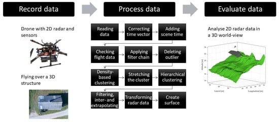
Thus, the main goal of this methodological approach was to develop a data processing pipeline to reconstruct a real-world scenario from radar measurements. To achieve this goal, the measurement system and location of the scenario were presented and data acquired from previous research [41] were used to show the results of a total of four flights. The data processing pipeline has a total of eleven stages. For this, we resorted to a common method called “density-based clustering”, presented in [49]. Finally, it will be worthwhile to highlight the results linked to the main advantages but also some limitations found regarding future applications in geosciences research.
2. Materials and Methods
2.1. Measurement System and Location
For this research, we used a measurement system built upon our previous research [41]. It consists of a radar sensor and a Raspberry Pi 3 Model B (RPi) with several connected sensors. The RPi is a small but powerful single-board computer. Due to a new UAV, a modified bracket was designed to attach the measurement system to the UAV.
The UAV is a self-made light quadcopter with a basic frame from Tarot called Iron Man FY650. As a flight controller, we used the Pixhawk 4 [50] from Holybro. It was programmed with the open-source autopilot software ArduPilot [51]. For the ground control station, we used the software Mission Planner. This allows us to automate flight routes by the UAV to ensure that the results are reproducible and repeatable. To power the UAV, a 6s battery with 5000 mAh was used, which enables flight times of around 15 min. With a 10,000 mAh battery, the flight time can be extended to 25 min. To achieve flight times beyond 30 min, a fixed wing UAV as presented in [19] should be used. The balancer connector of the battery, normally used to balance each cell while loading, was used to power the measurement system. In total, the UAV weighs around 2.4 kg including the battery and measurement system. The UAV is shown in Figure 1.
To assess the later transformation process, we selected a winery located in a vineyard. It is located in the southeast of Bingen am Rhein, Germany, on the south side of the Rochusberg (49.9592N, 7.9124E). Figure 2 shows an image from a flight over the building and a frontal picture. Advantages of the building are the structure as well as the seclusion, with good accessibility.
During the flight, the radar faces down and scans the ground. The flights were performed crossing over the building, which meant from the south to the north or vice versa. The microwaves propagate and expose a narrow rectangular area on the ground, subsequently referred to as a row. The area extends perpendicular to the flight direction of the UAV. The height and width of the measured area depend on the azimuth aperture angle of the radar and the elevation angle, respectively. Only the azimuth angle is measured by the radar, and not the small elevation angle. The radar sensor measures only in two dimensions, the azimuth angle or width and the distance to the object.
2.2. Data Acquisition
For the data acquisition part, the results from our previous work were used. In our previous research [41], we demonstrated how to record data with an automotive radar sensor called ARS-408 from Continental [52], which we also used for this research. The price for the sensor is around EUR 2500 for research purposes, but the unit cost drops when buying in larger quantities (e.g., the unit cost for ten sensors is EUR 900) [53]. We chose this sensor as it is the only radar sensor that meets our requirements: low weight, small size, easy-to-use data interface and an affordable price. As an additional advantage, the sensor is able to pre-process radar data, which enables those with no prior experience with radar data interpretation to evaluate the data. Due to this, the focus of this research lies on the process after classical radar data processing. Thereby, we process the recorded data on a normal workstation.
The output of the radar is called cluster data and can be represented as a point cloud. These clusters represent microwave reflections from the objects scanned by the radar sensor. An object’s reflection depends on the distance and orientation to the radar, as well as the size and material of the object. For these reasons, every object has a different reflection. The strength of the reflection is measured in m2 or dBm2 and is called the radar cross-section (RCS). The higher the RCS value of an object, the more detectable it is. For example, a human has around 1 m2 and a car around 100 m2. The maximum output of the ARS-408 is 256 clusters with a refresh rate of 60 ms. The number of clusters depends on the surroundings and the radar sensor setup, which is specified in Table 1.
A single cluster of the radar is specificized by a longitudinal (x) and lateral (y) position [41]. Further information of a cluster includes the RCS value and the velocity. The basic information of a cluster is shown in Table 2. The radar sensor does not provide a velocity on the lateral axis, but the value is in the message and always zero. The dynamic property specifies if the cluster is, e.g., moving or stationary. Further, a separate message can be used to obtain quality information for each cluster. Therewith, advanced filtering is possible to exclude possible incorrect clusters.
A measurement over time results in a cluster cloud. Thereby, time is the third dimension besides the x and y position of the radar. The point cloud is comparable to that of a Light Detection and Ranging (LiDAR) sensor, as shown in [54]. In contrast to LiDAR, the characteristics of the measurement differ and the radar clusters are not as sharp and accurate as LiDAR points, because of the microwave spread. Therefore, the data processing needs to be different. Besides the radar data, other sensors will be recorded and used for the evaluation. The radar data are recorded by the RPi and stored in a CSV file. Further, there is a global navigation satellite system (GNSS), inertial measurement unit (IMU) and temperature and pressure sensors connected to the RPi as well. GNSS is the super class of the famous Global Positioning System (GPS) but also of the Galileo system of the European Union. The IMU is a combination of two or three sensors: accelerometer, gyroscope and sometimes a magnetometer. The values of these sensors will be recorded in a different CSV file. Additionally, we used a small Raspberry Camera V2 to take pictures while recording. The radar sensor cluster clouds are difficult to interpret and therefore the camera pictures are used to identify them. The last dataset is recorded by the flight controller, which saves all sensors such as GNSS, IMU and pressure, as well as further flight information. Thus, there is redundancy of data, which is used to average sensor values and detect errors or malfunctions of the sensors. These two datasets differ only by the sensor type and the recording data rate.
2.3. Data Processing
As the authors of [41] described, the radar sensor data require processing in order to separate the value data from the noise or ghost data, as well as a transformation into the 3D world. Therefore, we designed the following independent processing steps.
- Reading data from CSV file;
- Correcting time vector and adding scene time;
- Checking if the flight is suitable for evaluation;
- Applying filter chain;
- Deleting outlier radar data;
- Applying density-based clustering;
- Stretching the cluster perpendicular to the ground plane;
- Applying hierarchical clustering;
- Filtering, inter- and extrapolating sensor data;
- Transforming 2D radar data into 3D;
- Fitting cluster to a surface.
Each step operates on the data of its predecessor. The following sections describe the respective function in detail. To use the results of this work with a different measurement setup, only the first step needs to be adjusted.
2.3.1. Reading Data
Excluding the camera data, all data were loaded from the CSV files and saved into vectors or matrices and stored in the following structures:
- Radar sensor (RAD)—signals listed in Table 2;
- RPi sensors—GNSS, IMU, temperature and pressure;
- UAV sensors—GNSS, IMU and pressure.
2.3.2. Correcting and Adding Time
Usually, all structures contain different time vectors due to different recording times and measurement intervals. Furthermore, the UAV has a different time vector for each sensor. Because of this, the inequalities (1) can be defined. Additionally, the numbers of elements (cardinality) are all different, as shown in Equation (2).
Due to this, all time vectors may need to be corrected. To align all measurements, a salient change in the pitch was used, which can be identified as a peak in all datasets. In Figure 3, the radar data (blue) of three pitch movements are shown. Further, the pitch values of the sensors from the RPi (green) and UAV (red) are indicated. Even though the radar and RPi show only a slight difference, these three datasets are not synchronous. The radar time is used as the reference time and the two others were corrected. To do this, the maximum was determined in all three datasets. This means that the maximum of the longitudinal axis (x-axis) vector was searched in the radar data and the corresponding timestamp of this single cluster was determined. For the RPi, the maximum pitch angle (y-axis) of the IMU was identified. The same process was used for the UAV pitch angle. The following timestamps were determined for the example shown in Figure 3a:
- Radar = 35.8109 s;
- RPi = 35.6997 s;
- UAV = 511.761 s.
Subsequently, the correction can be applied. As already mentioned, the radar time vector was used as a reference and will not be changed. Therewith, the time of the RPi was adjusted by adding the time of the maximum from the radar and subtracting the time for the maximum of the RPi. The time-corrected result is shown in Figure 3b. Afterwards, negative values and values exceeding the maximum radar time can be deleted or ignored. Therewith, the following definition applies (see Equation (3)).
The camera data are excluded from this process. An accurate synchronous time is not necessary to be conducted because we only used the camera data as a reference and did not merge them with other measurements. Furthermore, the camera time is nearly synchronous with the RPi time. Another option is to use a video stream, as the peak of the pitch movement used for the time correction can be detected with image processing.
The last step of this process is to limit the scene time. Since the measurement system records continuously, the vectors and matrices can become very long. This will cause longer processing times, while most of the data are not of interest. To increase the performance of further processes, the beginning and end of the parts of interest were searched with the help of the camera pictures and sensor data. The rest of the data were discarded and the start and stop times of the relevant parts were stored.
2.3.3. Checking Flight Data
To analyze the influence of the movement from the UAV on the radar data, the sensor data were analyzed. For this, we calculated the mean, standard deviation, skewness and integral. The mean value indicated whether the flight was smooth or not. With the standard deviation, we verified that there were no major influences such as wind gusts during the flight. The skewness indicated whether the data increased or decreased over the measurement time due to other influences such as sensor errors. The integral was used to determine whether the UAV had a drift caused by a strong permanent wind. To calculate the integral of the sensor data, we used a numerical trapezoidal method. For this, the time vector and the sensor data vector were used. The values of the latter were further converted into absolute values, so that negative outliers could not compensate positive ones.
2.3.4. Filter Chain
To prepare the radar data, several filters were applied. First, we limited the x- and y-axis. On the longitudinal axis, the minimum and maximum values of the radar sensor are 0 and 194 m, respectively. The range of interest needs to contain the ground and the building. With a flight altitude of around 20 m, this leads to a range of approximately 10 to 30 m. To determine an appropriate range, a histogram can be helpful, as Figure 4a shows. Further, the lateral values are limited to −15 to +15 m. Depending on the height of the flight, some objects may not be detected as they lie behind other ones. This effect is called radar shadow. Because of this, it is not useful to choose high lateral ranges such as −80 to +80 m. The winery is around 13 m wide and so the chosen limit is suitable. The values are not easy to identify in the histogram, as shown in Figure 4b. Due to this, it is helpful to know the object location and dimensions to avoid searching the unfiltered data.
The same process was carried out for the RCS value and the longitudinal velocity. Next, we used the quality information of each cluster to have additional filter options. Thereby, it must be noted that the filtering can quickly become too narrow. This means that not only noisy clusters will be deleted, but also useful data. Therefore, it is advisable to use soft filtering at the start and use this filter chain again at the later stage of the data processing with a tighter filter setup when necessary.
2.3.5. Delete Outlier Radar Data
Due to basic radar reflection errors, several ghost clusters can be found in the dataset. These clusters are often located in unrealistic locations, such as in the air next to the UAV. To find and delete these outliers, we designed a filter algorithm. Therefore, a filter cuboid was defined that is characterized by time, longitude and latitude. These three values are corresponding to the three-dimensional radar axis. The algorithm iterates over all clusters, and for each cluster, the neighborhood is determined with the cuboid. All clusters that are located in the cuboid are counted and compared with a defined number of minimum required clusters. If the counted number is smaller than the defined number of minimum clusters, the tested cluster will be marked and deleted at the end of the process. This means that, for the whole process, all clusters will be used, even if the cluster was already marked as deleted. The filter algorithm works in the following seven steps:
- Define the cuboid by time, longitude and latitude;
- Define the minimum number of clusters;
- Set the cuboid to the first cluster, so that is lies in its center;
- Count all clusters in the cuboid;
- If the number of minimum clusters is not reached, mark the current cluster;
- Iterate over all clusters and repeat steps 4 and 5;
- Delete all marked clusters.
2.3.6. Density-Based Clustering
To separate required clusters from noise clusters, a density-based spatial clustering algorithm described in [49] was used with a run time complexity of O(n log n). This is possible because the noise clusters or sometimes ghost clusters accumulate on separate hot spots in a distance to the required clusters. The algorithm needs an epsilon distance and a number to specify the minimum number of clusters. It starts with the first cluster, which will be labeled and assigned to the first group. If this cluster has fewer neighbors than the defined number of minimum clusters, this cluster will be labeled as noise. Otherwise, the cluster will be labeled as a core point. All clusters in the epsilon distance to this cluster are its neighbors. All neighbors will then be tested and also categorized as noise or a core point. Neighbors labeled as a core point will be assigned the same group as the starting core point. After all neighbors are processed, the next unlabeled cluster will be tested but will be assigned to a new group. This is repeated until no more clusters are left.
The result is that all dense cluster clouds are now labeled and belong to a group. Therewith, noise groups can be deleted and the remaining cluster clouds can be used for further processing.
2.3.7. Cluster Stretching
For our goal, it is important to reliably detect leaps in height between the different clusters in order to identify objects within the measurement data. As most common clustering algorithms use spherical distance methods to determine groups, we stretched our radar data perpendicular to the ground plane to allow improved height differentiation while keeping the distances of all other axes unchanged.
To do this, we computed the plane from the radar data that had the smallest overall distance to all radar points. Note that this method is only practical if the ground plane covers most of the measurement or if the height of all objects is almost evenly distributed across the measurement. Otherwise, the stretching axis will not be perpendicular to the original scene’s ground plane, thus probably leading to erroneous results. In these cases, a more sophisticated algorithm or manual adjustment will be required.
The calculation of the plane is done with a polynomial fitting algorithm using only one degree of freedom for each axis. Equation (4) shows the function to calculate the height z of a plane at a certain coordinate described by x and y. The constants , and define the orientation of the plane in 3D space and have to be determined.
The calculation of the constants is performed by creating a system of linear equations by inserting the measured cluster data, each represented by , and , into the function and then applying the linear squares method. Equation (5) shows the matrix containing the x- and y-coordinates, the vector containing the searched constants and the vector containing the z-coordinates. In Equation (6), the linear squares method is shown.
The resulting plane formula can then be used to calculate a perpendicular vector. First, two vectors on the plane are constructed by inserting the points (0, 0), (0, 1) and (1, 0) into the formula and subtracting the resulting value of the first point from each of the latter two. Since our goal is only to create a perpendicular vector to the plane, the two calculated vectors do not have to be orthogonal to each other. Next, the perpendicular vector can be calculated by determining the cross product of the two vectors.
All cluster points can then be stretched along the normal vector by adding a multiple to their coordinates. The scalar defining how many times the normal is added will later again be used to restore the original positions.
2.3.8. Hierarchical Agglomerative Distance-Based Clustering
To separate the cluster data of the ground plane from the objects of interest, we used a hierarchical agglomerative distance-based clustering algorithm with a complexity of O (n3) [55]. By stretching the data before, we enhanced the detection of clusters and reduced the influence of outliers, which can also be neglected here as we already eliminated most of them, as described in Section 2.3.6.
The used algorithm is threefold. First, the distance between all points of the dataset is calculated by using the Euclidean distance. Afterwards, the resulting distances are used to create a binary hierarchical cluster tree in an agglomerative way. For this, each point is first assigned its own cluster, which then is iteratively linked pairwise depending on their proximity. We used the centroid to calculate the position of the created groups by calculating the average position of all contained points and used it again to determine the distance to other elements. All grouping steps are logged and the process is done until all points are grouped into one large set. This grouping process is often visualized using a dendrogram, which does not only show the resulting clusters but also all sub-steps. An exemplary diagram for the clustering of radar data can be seen in Figure 5.
The third step of the algorithm is then to determine in which height to cut the binary tree to achieve the desired clustering. We used a max cluster approach for this as we can narrow down the clusters to identify with the knowledge of the measured scene. Hereby, the binary tree will be cut at several levels, starting from the root. The final result is the lowest level where the maximum number of clusters is not exceeded.
2.3.9. Filter and Interpolate Sensor Data
To prepare the transformation from the two-dimensional radar data into the three-dimensional world, the sensor data need to be filtered and interpolated. This is necessary because: (i) some sensors have a low data rate, e.g., the GNSS data rate is 5 Hz; (ii) with this process, we ensure that the radar data time points accurately match the sensor data time points; and (iii) the noisy sensor data are smoothed for a soft transformation without sudden jumps. The low data rate of some sensors should not be confused with the basic recording data rate. In comparison to the high data rate of the radar sensor, which is 16.6 Hz, the low GNSS rate will lead to a striped pattern of the data after the transformation process. Therefore, the low sensor data rate will be interpolated up to the high data rate of the radar.
Before performing the interpolation, we filtered the GNSS, IMU and pressure data with a moving mean filter. The filter window, describing the number of used values for the mean, was adjusted to the sensor by an empirical method. After filtering, the interpolation was performed. For this, the vectors need to be unique values and strictly monotonic. As a result, duplicate GNSS data were deleted. It is important to note that this part of the algorithm was only used for GNSS sensors with a low data rate. Sensors with a higher data rate do not need to undergo these steps.
For the algorithm, we used a linear interpolation method that requires at least two points. The length of the output vector of the interpolation was often shorter than the input vector. The missing values are at the beginning and end of the vector. To keep the vectors in the same length and avoid consequent problems in further processing, additionally, extrapolation was performed. With this last step, the sensor data were prepared for the next step.
2.3.10. Transform 2D Radar Data into 3D
To transform the two-dimensional radar data into the three-dimensional world, we used the GNSS and IMU sensor data. The radar axes longitudinal (x) and lateral (y) are dependent on the time t so they can be defined as discrete functions x(t) and y(t). Due to the time accuracy of the prepared sensor data, the corresponding sensor value to each t is known. To combine the radar and the GNSS data, first, the GNSS data need to be transformed from geodetic coordinates in degrees to the so-called “flat Earth” coordinates in meters. For this, a reference GNSS point is necessary to define the origin of the flat Earth coordinates, e.g., the take-off position. Further, the longitudinal and lateral axes of the radar are now renamed to match with the axes of the three-dimensional world. This means that the radar longitudinal is renamed to altitude and the radar lateral is now called longitudinal. The lateral value of the radar is initially set to zero and later corrected by applying the GNSS position. The correction must be postponed to allow the correct rotation of the data beforehand.
Next, the radar data are rotated by the roll, pitch and yaw angle of the drone to properly reconstruct the coordinates of the separate clusters. To ease the later processing, we calculated a matrix representing a basis transformation from the drone to the world coordinates for each discrete time step. To achieve this, we first constructed the matrix representing the drone’s alignment by multiplying the three rotation matrices , and defined by the yaw, pitch and roll value, respectively. By defining the world’s orientation matrix as the identity matrix , the transformation matrix is equal to the rotation matrix of the drone. The several definitions are highlighted in Equations (7) and (8), which show the calculation of the transformation matrix that will be applied from the left to the cluster data of the given point in time.
After rotating all clusters, the GNSS information is added to the radar data. To each radar point, now described by lateral, longitudinal and altitude, the GNSS information that corresponds to the specific time will be added.
After the transformation process, the ground level is at altitude zero. This is because of the altitude reference of the take-off position. If necessary, the mean flight altitude can be added. Therewith, the UAV is on altitude zero and the ground level is on the distance to the UAV.
2.3.11. Fit Cluster to a Surface
This last step is not used for processing the data, but only for the presentation of the data. To do this, we interpolated a finite element surface for each radar data cluster of interest. Then, we used a local linear regression algorithm, which uses a weighted least squares algorithm similar to the one described in Section 2.3.7. Different to the algorithm used for plane fitting, individual planes are computed for each input point by only taking into account certain neighbor points. The more points are used for the calculation, the more the resulting surface approaches a plane fit.
3. Results
To evaluate the process presented above, we used measurements of the example scene with different flight parameters (see Table 3).
We show that by applying the steps proposed, it is possible to identify objects from the radar data. Different flights show that an altitude of around 20 m and a flight velocity of around 1 m/s are most suitable. A higher altitude results in fewer clusters and a faster velocity leads to the blurring of objects that are close to each other in the direction of the flight.
The RCS threshold parameter of the radar was tested but did not improve the results. The high sensitivity mode leads to much more clusters but also increases the noise dramatically. In our case, after the density-based clustering, the number of clusters was the same for the high and normal sensitivity modes.
After the initial data reading and correction, we verified the flight data. While observing these values, we detected that the IMU BNO055 sometimes drifts on the roll or pitch axis, which results in high skewness of these data. To verify that the sensor works properly, we installed an additional IMU from WitMotion called WT901 [56] to the system. Therewith, we obtained three IMUs and could determine whether one IMU had a malfunction. For further processing, we used flights with appropriate values, which were flights without heavy wind or gusts.
Next, we performed the first filtering of the radar data. First, we extracted one flight over the building from the complete flight. Then, we limited the longitudinal and lateral axes as well as the RCS value. These limits were set loosely, so that we did not delete important data in this early stage. In the next steps, we deleted the outliers and performed density-based clustering. Both methods are used to eliminate incorrect radar cluster data. The parameters of the methods need to be adjusted for different flight or radar parameters.
Afterwards, the clusters were stretched to ensure an accurate result when separating the building from all other clusters. We identified that 1000 is a good and stable stretching factor for all measurements. After this, we used hierarchical agglomerative distance-based clustering to extract the building data. Thereby, this process shows some instability. To obtain proper results, the max cluster parameter must be adjusted. Afterwards, the radar data must be compressed by the same factor as for stretching.
Next, the radar data of the building were filtered again by the filter chain. In addition to the filter values of the first filtering, we used the dynamic property and longitudinal velocity. Filtering by the velocity results in the sharpening of the data in the direction of the flight, which is important to reconstruct the correct dimensions of the building. This same process was carried out with the ground radar cluster data, but more filters and even narrower limits were used. Depending on the quality of the flight, additional noise reduction, as described in Section 2.3.5 and Section 2.3.6, may be required for the building data.
After these steps, we have separated the building from the ground and even from noisy clusters. Figure 6a shows the building from the top and Figure 6b from the front (compare to Figure 2). The clusters within the black lines are not from the outer walls of the building, but from the rooftop. Now, the dimensions of the building can be determined. Table 4 shows the real dimensions and those extracted from four flights.
Because of the location of the winery in uneven terrain, the height to the ground is different on the left and right sides. To calculate the width, which is the time axis at this stage, we used the mean GNSS velocity to calculate the width in meters.
The width has the highest deviation. As mentioned earlier, higher flight velocities reduce the width accuracy. The other dimensions match the real dimensions and deviate by around 0.2 to 0.4 m. Thereby, it must be considered that the radar data have only an output resolution of 0.2 m. This means that the deviation is only one to two times the resolution.
In the next step, the sensor data were prepared for transformation into a three-dimensional world. Thereby, the sensor values were filtered as well as inter- and extrapolated. After this, we transformed the basis and added the GNSS information. For the altitude, we used the barometer information because it showed better results than the GNSS altitude. However, the GNSS altitude was used to determine the start altitude over sea level. Therewith, the data processing is complete and the dimensions of the building can be determined, including the sensor information. Table 5 shows the measured values.
Except for the width, these values show a similar deviation as the results in Table 4. The width has improved and depicts a lower deviation.
The last step is to create figures with a surface, as shown in Figure 7. Only the ground (green), rooftop (grey) and the top of the chimney (silver) are visible.
A flight scene over the building counts around 25,000 clusters for the normal sensitivity mode and around 50,000 for the high sensitivity mode. After complete processing, the building counts approximately 370 clusters and the ground around 3000 regardless of the choice of sensitivity. This represents a reduction of around 86% for the normal sensitivity mode and 93% for the high sensitivity mode. Therewith, the high sensitivity mode has no added value for this application. The assumption that this mode would provide more and thus better results was therefore not confirmed. This could be due to the fact that the error rate increases with this mode, which leads to more clusters being filtered.
4. Discussion and Further Challenges
The paper presents a dedicated data processing pipeline to reconstruct a three-dimensional scenario from the data of a low-cost radar sensor. The data processing is well organized but still needs manual work such as identifying the key objects of the scenario in the dataset, time synchronization of the different data or finding suitable parameters for the hierarchical and density-based clustering. To separate the objects from the ground, we stretch the data perpendicular to the ground beforehand. This process step is only possible for scenarios where the ground radar data contain many more data points as the object.
The radar data are outputted in a 0.2 m resolution. The results show that most measurements are two or three times this resolution. This means that objects with a size of 0.4 to 0.6 m can be definitively detected. For smaller objects, the chosen radar sensor is unsuitable, because there is no configuration possible to increase the accuracy. Therefore, other methods, such as Structure from Motion, should be combined to provide this information [57,58,59]. Further, this resolution can be more limited by a turbulent flight. For example, an uncompensated or incorrect roll angle of just 1° at a flight altitude of 30 m results in a difference on the ground of around 0.5 m. Higher demands cannot be met with the relatively cheap sensors that were used in this research. This shows that the precision of the sensors and the radar sensor are compatible and that a higher radar resolution requires a higher sensor standard.
The proposed flight parameters with 20 m flight altitude and 1 m/s flight velocity are suitable for most applications. For applications with a low-resolution requirement, a higher altitude and a faster velocity is possible. As already mentioned, a higher flight altitude leads to fewer clusters per object and a faster velocity leads to a blurring effect in the direction of the flight. For unknown object detection, it might be useful to perform two flights—the first one in a low-resolution mode to obtain an overview of the scenario and the second one in a high-resolution mode to scan only the important part of the scenario.
The determination of the object dimensions—in this research, a building—with the radar cluster data is difficult, because they are not on an equidistant grid. Therewith, it could be necessary to use two cluster points that are not perfectly positioned to measure a distance. A solution is to fit the cluster to a surface, as shown in Figure 7, which makes the measurement much easier. Nevertheless, this surface can be inaccurate if the radar data are strongly fluctuating. Further, the radar shadow prevents the direct measurement of the height, because there may be no ground clusters visible while flying directly above the winery.
As described, the radar sensor has no precise resolution in the direction of flight. Therefore, the radar beam blurs the objects on the ground in this direction. This can be corrected by filtering the velocity but is only applicable for slow flight velocities. Further, with a faster flight velocity, the radar creates too few clusters of an object. This can be compensated with an overlay of several measurements, but for this, several flights are necessary.
The RCS threshold setup of the radar sensor should increase when detecting small and less strongly reflecting objects. In this research, the high sensitivity mode has no impact, except for an increase in noise.
In this work, we focused on the feasibility of three-dimensional reconstruction in a processing phase subsequent to the measurement. The choice of algorithms therefore fell on those with the best results, although these had higher complexity than others. Especially for direct processing of the data, some algorithms would have to be adapted, optimized or even replaced. In addition, a simple pre-filtering is possible, to reduce the data during the flight.
5. Conclusions
This research shows that the combination of a UAV and low-cost radar sensor from the automotive field is suitable to reconstruct a three-dimensional scenario. We introduced a measurement system, the radar sensor, and proposed a processing pipeline with eleven stages in total to recover the scenario. To verify the data processing, we applied it to measurements of a building in a vineyard. The results showed that most measurements have a deviation of around 0.4 to 0.6 m. The resolution depends not only on the radar sensor, but also on the additional sensors, e.g., IMU and GNSS.
Further research will focus on a new radar sensor called ARS-540 from the automotive field. This sensor has several advantages, such as three-dimensional detection, an extended setup possibility and a higher resolution. We expect increasing performance, independent measurement and a wider range of applications.
Author Contributions
Conceptualization, C.W.; methodology, C.W. and M.E.; software, C.W. and M.E.; formal analysis, M.E.; investigation, C.W.; data curation C.W.; writing—original draft preparation C.W., M.E. and J.R.-C.; writing—review and editing, T.U.; visualization, J.R.-C. and T.U.; project administration, C.W. All authors have read and agreed to the published version of the manuscript.
Funding
This research received no external funding.
Institutional Review Board Statement
Not applicable.
Informed Consent Statement
Not applicable.
Data Availability Statement
The data used to support the findings of this study are available from the corresponding author upon request.
Acknowledgments
This research work was supported by the “European Regional Development Fund” (EFRE) in the context of the aim of “Investment in Growth and Employment” (IWB) in Rhineland-Palatinate, Germany.
Conflicts of Interest
The authors declare no conflict of interest.
References
- Applications of Unmanned Aerial Vehicles in Geosciences. Available online: https://link.springer.com/book/9783030031701 (accessed on 2 January 2022).
- Kyriou, A.; Nikolakopoulos, K.; Koukouvelas, I.; Lampropoulou, P. Repeated UAV Campaigns, GNSS Measurements, GIS, and Petrographic Analyses for Landslide Mapping and Monitoring. Minerals 2021, 11, 300. [Google Scholar] [CrossRef]
- Gawehn, M.; De Vries, S.; Aarninkhof, S. A Self-Adaptive Method for Mapping Coastal Bathymetry On-The-Fly from Wave Field Video. Remote Sens. 2021, 13, 4742. [Google Scholar] [CrossRef]
- Chen, J.; Sasaki, J. Mapping of Subtidal and Intertidal Seagrass Meadows via Application of the Feature Pyramid Network to Unmanned Aerial Vehicle Orthophotos. Remote Sens. 2021, 13, 4880. [Google Scholar] [CrossRef]
- Mogili, U.R.; Deepak, B.B.V.L. Review on Application of Drone Systems in Precision Agriculture. Procedia Comput. Sci. 2018, 133, 502–509. [Google Scholar] [CrossRef]
- Khun, K.; Tremblay, N.; Panneton, B.; Vigneault, P.; Lord, E.; Cavayas, F.; Codjia, C. Use of Oblique RGB Imagery and Apparent Surface Area of Plants for Early Estimation of Above-Ground Corn Biomass. Remote Sens. 2021, 13, 4032. [Google Scholar] [CrossRef]
- Al-Naji, A.; Perera, A.G.; Mohammed, S.L.; Chahl, J. Life Signs Detector Using a Drone in Disaster Zones. Remote Sens. 2019, 11, 2441. [Google Scholar] [CrossRef] [Green Version]
- Hildmann, H.; Kovacs, E. Review: Using Unmanned Aerial Vehicles (UAVs) as Mobile Sensing Platforms (MSPs) for Disaster Response, Civil Security and Public Safety. Drones 2019, 3, 59. [Google Scholar] [CrossRef] [Green Version]
- Wufu, A.; Yang, S.; Chen, Y.; Lou, H.; Li, C.; Ma, L. Estimation of Long-Term River Discharge and Its Changes in Ungauged Watersheds in Pamir Plateau. Remote Sens. 2021, 13, 4043. [Google Scholar] [CrossRef]
- Wufu, A.; Chen, Y.; Yang, S.; Lou, H.; Wang, P.; Li, C.; Wang, J.; Ma, L. Changes in Glacial Meltwater Runoff and Its Response to Climate Change in the Tianshan Region Detected Using Unmanned Aerial Vehicles (UAVs) and Satellite Remote Sensing. Water 2021, 13, 1753. [Google Scholar] [CrossRef]
- D’Oleire-Oltmanns, S.; Marzolff, I.; Peter, K.D.; Ries, J.B. Unmanned Aerial Vehicle (UAV) for Monitoring Soil Erosion in Morocco. Remote Sens. 2012, 4, 3390–3416. [Google Scholar] [CrossRef] [Green Version]
- Candiago, S.; Remondino, F.; De Giglio, M.; Dubbini, M.; Gattelli, M. Evaluating Multispectral Images and Vegetation Indices for Precision Farming Applications from UAV Images. Remote Sens. 2015, 7, 4026–4047. [Google Scholar] [CrossRef] [Green Version]
- Yin, N.; Liu, R.; Zeng, B.; Liu, N. A review: UAV-based Remote Sensing. IOP Conf. Ser.: Mater. Sci. Eng. 2019, 490, 062014. [Google Scholar] [CrossRef]
- Adamopoulos, E.; Rinaudo, F. UAS-Based Archaeological Remote Sensing: Review, Meta-Analysis and State-of-the-Art. Drones 2020, 4, 46. [Google Scholar] [CrossRef]
- Manfreda, S.; McCabe, M.F.; Miller, P.E.; Lucas, R.; Madrigal, V.P.; Mallinis, G.; Ben Dor, E.; Helman, D.; Estes, L.; Ciraolo, G.; et al. On the Use of Unmanned Aerial Systems for Environmental Monitoring. Remote Sens. 2018, 10, 641. [Google Scholar] [CrossRef] [Green Version]
- Koh, L.P.; Wich, S.A. Dawn of Drone Ecology: Low-Cost Autonomous Aerial Vehicles for Conservation. Trop. Conserv. Sci. 2012, 5, 121–132. [Google Scholar] [CrossRef] [Green Version]
- Naughton, J.; McDonald, W. Evaluating the Variability of Urban Land Surface Temperatures Using Drone Observations. Remote Sens. 2019, 11, 1722. [Google Scholar] [CrossRef] [Green Version]
- Prasenja, Y.; Alamsyah, A.T.; Bengen, D.G. Land-Use Analysis of Eco Fishery Tourism Using a Low-Cost Drone, the Case of Lumpur Island, Sidoarjo District. IOP Conf. Ser. Earth Environ. Sci. 2018, 202, 012014. [Google Scholar] [CrossRef]
- Von Eichel-Streiber, J.; Weber, C.; Rodrigo-Comino, J.; Altenburg, J. Controller for a Low-Altitude Fixed-Wing UAV on an Embedded System to Assess Specific Environmental Conditions. Int. J. Aerosp. Eng. 2020, 2020, 1360702. [Google Scholar] [CrossRef]
- Remke, A.; Rodrigo-Comino, J.; Wirtz, S.; Ries, J. Finding Possible Weakness in the Runoff Simulation Experiments to Assess Rill Erosion Changes without Non-Intermittent Surveying Capabilities. Sensors 2020, 20, 6254. [Google Scholar] [CrossRef]
- Caduff, R.; Schlunegger, F.; Kos, A.; Wiesmann, A. A review of terrestrial radar interferometry for measuring surface change in the geosciences. Earth Surf. Process. Landforms 2015, 40, 208–228. [Google Scholar] [CrossRef]
- Smith, L.C. Emerging Applications of Interferometric Synthetic Aperture Radar (InSAR) in Geomorphology and Hydrology. Ann. Assoc. Am. Geogr. 2002, 92, 385–398. [Google Scholar] [CrossRef]
- GPR Applications across Engineering and Geosciences Disciplines in Italy: A Review. Available online: https://ieeexplore.ieee.org/abstract/document/7475886/ (accessed on 2 January 2022).
- Samaras, S.; Diamantidou, E.; Ataloglou, D.; Sakellariou, N.; Vafeiadis, A.; Magoulianitis, V.; Lalas, A.; Dimou, A.; Zarpalas, D.; Votis, K.; et al. Deep Learning on Multi Sensor Data for Counter UAV Applications—A Systematic Review. Sensors 2019, 19, 4837. [Google Scholar] [CrossRef] [PubMed] [Green Version]
- Bethke, K.-H.; Baumgartner, S.; Gabele, M. Airborne Road Traffic Monitoring with Radar. In Proceedings of the World Congress on Intelligent Transport Systems (ITS), Beijing, China, 9–13 October 2007; pp. 1–6. Available online: https://elib.dlr.de/51746/ (accessed on 25 February 2022).
- Besada, J.A.; Campaña, I.; Carramiñana, D.; Bergesio, L.; De Miguel, G. Review and Simulation of Counter-UAS Sensors for Unmanned Traffic Management. Sensors 2022, 22, 189. [Google Scholar] [CrossRef]
- Coluccia, A.; Parisi, G.; Fascista, A. Detection and Classification of Multirotor Drones in Radar Sensor Networks: A Review. Sensors 2020, 20, 4172. [Google Scholar] [CrossRef]
- Haley, M.; Ahmed, M.; Gebremichael, E.; Murgulet, D.; Starek, M. Land Subsidence in the Texas Coastal Bend: Locations, Rates, Triggers, and Consequences. Remote Sens. 2022, 14, 192. [Google Scholar] [CrossRef]
- De Alban, J.D.T.; Connette, G.M.; Oswald, P.; Webb, E.L. Combined Landsat and L-Band SAR Data Improves Land Cover Classification and Change Detection in Dynamic Tropical Landscapes. Remote Sens. 2018, 10, 306. [Google Scholar] [CrossRef] [Green Version]
- Bauer-Marschallinger, B.; Paulik, C.; Hochstöger, S.; Mistelbauer, T.; Modanesi, S.; Ciabatta, L.; Massari, C.; Brocca, L.; Wagner, W. Soil Moisture from Fusion of Scatterometer and SAR: Closing the Scale Gap with Temporal Filtering. Remote Sens. 2018, 10, 1030. [Google Scholar] [CrossRef] [Green Version]
- Sivasankar, T.; Kumar, D.; Srivastava, H.S.; Patel, P. Advances in Radar Remote Sensing of Agricultural Crops: A Review. Int. J. Adv. Sci. Eng. Inf. Technol. 2018, 8, 1126–1137. [Google Scholar] [CrossRef] [Green Version]
- Nikaein, T.; Iannini, L.; Molijn, R.A.; Lopez-Dekker, P. On the Value of Sentinel-1 InSAR Coherence Time-Series for Vegetation Classification. Remote Sens. 2021, 13, 3300. [Google Scholar] [CrossRef]
- Lausch, A.; Bastian, O.; Klotz, S.; Leitão, P.J.; Jung, A.; Rocchini, D.; Schaepman, M.E.; Skidmore, A.K.; Tischendorf, L.; Knapp, S. Understanding and assessing vegetation health by in situ species and remote-sensing approaches. Methods Ecol. Evol. 2018, 9, 1799–1809. [Google Scholar] [CrossRef]
- Tripathi, A.; Tiwari, R.K. Utilisation of spaceborne C-band dual pol Sentinel-1 SAR data for simplified regression-based soil organic carbon estimation in Rupnagar, Punjab, India. Adv. Space Res. 2021, 69, 1786–1798. [Google Scholar] [CrossRef]
- Liu, Y.; Wang, H.; Lei, X. Real-time forecasting of river water level in urban based on radar rainfall: A case study in Fuzhou City. J. Hydrol. 2021, 603, 126820. [Google Scholar] [CrossRef]
- Qi, Y.; Fan, S.; Li, B.; Mao, J.; Lin, D. Assimilation of Ground-Based Microwave Radiometer on Heavy Rainfall Forecast in Beijing. Atmosphere 2022, 13, 74. [Google Scholar] [CrossRef]
- Klotzsche, A.; Jonard, F.; Looms, M.; Van der Kruk, J.; Huisman, J. Measuring Soil Water Content with Ground Penetrating Radar: A Decade of Progress. Vadose Zone J. 2018, 17, 180052. [Google Scholar] [CrossRef] [Green Version]
- Giannakis, I.; Giannopoulos, A.; Warren, C. A Realistic FDTD Numerical Modeling Framework of Ground Penetrating Radar for Landmine Detection. IEEE J. Sel. Top. Appl. Earth Obs. Remote Sens. 2016, 9, 37–51. [Google Scholar] [CrossRef]
- Winner, H.; Hakuli, S.; Lotz, F.; Singer, C. (Eds.) Handbook of Driver Assistance Systems: Basic Information, Components and Systems for Active Safety and Comfort; Springer International Publishing: Berlin/Heidelberg, Germany, 2016; Available online: https://www.springer.com/de/book/9783319123516 (accessed on 27 February 2020).
- Reif, K. (Ed.) Brakes, Brake Control and Driver Assistance Systems: Function, Regulation and Components; Springer: Berlin/Heidelberg, Germany, 2014. [Google Scholar] [CrossRef]
- Weber, C.; Von Eichel-Streiber, J.; Rodrigo-Comino, J.; Altenburg, J.; Udelhoven, T. Automotive Radar in a UAV to Assess Earth Surface Processes and Land Responses. Sensors 2020, 20, 4463. [Google Scholar] [CrossRef]
- Siebert, S.; Teizer, J. Mobile 3D mapping for surveying earthwork projects using an Unmanned Aerial Vehicle (UAV) system. Autom. Constr. 2014, 41, 1–14. [Google Scholar] [CrossRef]
- Tagarakis, A.C.; Filippou, E.; Kalaitzidis, D.; Benos, L.; Busato, P.; Bochtis, D. Proposing UGV and UAV Systems for 3D Mapping of Orchard Environments. Sensors 2022, 22, 1571. [Google Scholar] [CrossRef]
- Nex, F.; Remondino, F. UAV for 3D mapping applications: A review. Appl. Geomat. 2014, 6, 1–15. [Google Scholar] [CrossRef]
- Gómez-Gutiérrez, Á.; Gonçalves, G.R. Surveying coastal cliffs using two UAV platforms (multirotor and fixed-wing) and three different approaches for the estimation of volumetric changes. Int. J. Remote Sens. 2020, 41, 8143–8175. [Google Scholar] [CrossRef]
- Vacca, G.; Furfaro, G.; Dessì, A. The Use of the Uav Images for the Building 3d Model Generation. ISPRS Int. Arch. Photogramm. Remote Sens. Spat. Inf. Sci. 2018, XLII-4/W8, 217–223. [Google Scholar] [CrossRef] [Green Version]
- Barba, S.; Barbarella, M.; Di Benedetto, A.; Fiani, M.; Gujski, L.; Limongiello, M. Accuracy Assessment of 3D Photogrammetric Models from an Unmanned Aerial Vehicle. Drones 2019, 3, 79. [Google Scholar] [CrossRef] [Green Version]
- Hugler, P.; Roos, F.; Schartel, M.; Geiger, M.; Waldschmidt, C. Radar Taking Off: New Capabilities for UAVs. IEEE Microw. Mag. 2018, 19, 43–53. [Google Scholar] [CrossRef] [Green Version]
- Ester, M.; Kriegel, H.P.; Sander, J.; Xu, X. A Density-Based Algorithm for Discovering Clusters in Large Spatial Databases with Noise. In Proceedings of the 2nd International Conference on Knowledge Discovery and Data Mining KDD-96, Portland, OR, USA, 2–4 August 1996; pp. 226–231. [Google Scholar]
- “Pixhawk 4” Holybro. Available online: http://www.holybro.com/product/pixhawk-4/ (accessed on 29 December 2021).
- ArduPilot “ArduPilot,” ArduPilot.org. Available online: https://ardupilot.org (accessed on 29 December 2021).
- “ARS 408” Continental Engineering Services. Available online: https://conti-engineering.com/components/ars-408/ (accessed on 4 January 2022).
- Cloos, C. Price Request ARS-408.
- Xia, S.; Chen, D.; Wang, R.; Li, J.; Zhang, X. Geometric Primitives in LiDAR Point Clouds: A Review. IEEE J. Sel. Top. Appl. Earth Obs. Remote Sens. 2020, 13, 685–707. [Google Scholar] [CrossRef]
- Day, W.H.E.; Edelsbrunner, H. Efficient algorithms for agglomerative hierarchical clustering methods. J. Classif. 1984, 1, 7–24. [Google Scholar] [CrossRef]
- WitMotion WT901 TTL & I2C Output 9 Axis AHRS Sensor Accelerometer + Gyroscope + Angle + Magnetic Field MPU9250. Available online: https://www.wit-motion.com/gyroscope-module/Witmotion-wt901-ttl-i2c.html (accessed on 5 January 2022).
- Kaiser, A.; Neugirg, F.; Rock, G.; Müller, C.; Haas, F.; Ries, J.; Schmidt, J. Small-Scale Surface Reconstruction and Volume Calculation of Soil Erosion in Complex Moroccan Gully Morphology Using Structure from Motion. Remote Sens. 2014, 6, 7050–7080. [Google Scholar] [CrossRef] [Green Version]
- Remke, A.; Rodrigo-Comino, J.; Gyasi-Agyei, Y.; Cerdà, A.; Ries, J.B. Combining the Stock Unearthing Method and Structure-from-Motion Photogrammetry for a Gapless Estimation of Soil Mobilisation in Vineyards. ISPRS Int. J. Geo-Inf. 2018, 7, 461. [Google Scholar] [CrossRef] [Green Version]
- Smith, M.W.; Vericat, D. From experimental plots to experimental landscapes: Topography, erosion and deposition in sub-humid badlands from Structure-from-Motion photogrammetry. Earth Surf. Process. Landf. 2015, 40, 1656–1671. [Google Scholar] [CrossRef] [Green Version]
Figure 1.
UAV based on Tarot Iron Man FY650 with flight controller Pixhawk 4, the battery and the complete measurement system.
Figure 1.
UAV based on Tarot Iron Man FY650 with flight controller Pixhawk 4, the battery and the complete measurement system.

Figure 2.
Winery located in the municipality of Bingen am Rhein, Germany, that was used to assess the transformation process. (a) Image from a flight over the building and (b) a front picture.
Figure 2.
Winery located in the municipality of Bingen am Rhein, Germany, that was used to assess the transformation process. (a) Image from a flight over the building and (b) a front picture.

Figure 3.
Example of time synchronization of three different sources by aligning their pitch movements. (a) Radar data (blue) are nearly synchronous with the pitch data of the RPi (green). The UAV pitch data (red) have different times. (b) Time-synchronized data.
Figure 3.
Example of time synchronization of three different sources by aligning their pitch movements. (a) Radar data (blue) are nearly synchronous with the pitch data of the RPi (green). The UAV pitch data (red) have different times. (b) Time-synchronized data.

Figure 4.
Histogram of the data from the flight over the building with an altitude of around 20 m. (a) Longitudinal axis, (b) lateral axis.
Figure 4.
Histogram of the data from the flight over the building with an altitude of around 20 m. (a) Longitudinal axis, (b) lateral axis.

Figure 5.
Dendrogram showing exemplary clustering of radar data. The diagram shows the created cluster hierarchy starting at a distance of 1000 m to ease visibility. All closer data points or cluster combinations are omitted. The blue horizontal connections represent the combination of two subclusters or values at a given distance. Note that the large distance of 1000 m resulted from the stretching process performed before.

Figure 6.
Reconstructed building with radar cluster data (blue points) and manually added building contours (black lines). Only the rooftop is visible. (a) View from the top, (b) view from the front.
Figure 6.
Reconstructed building with radar cluster data (blue points) and manually added building contours (black lines). Only the rooftop is visible. (a) View from the top, (b) view from the front.

Figure 7.
Reconstruction of the building after the complete processing pipeline. The ground is represented in green, the rooftop of the building in grey and the top of the chimney in silver.
Figure 7.
Reconstruction of the building after the complete processing pipeline. The ground is represented in green, the rooftop of the building in grey and the top of the chimney in silver.


Table 1.
Basic radar sensor setup, Continental ARS-408.
| Type | Value |
|---|---|
| Output type | Cluster |
| Send quality data | On |
| Maximum distance | 196 m |
| RCS threshold | Normal/high sensitivity |
Table 2.
Basic information of a single cluster, of the radar sensor Continental ARS-408.
| Signal | Description | Unit |
|---|---|---|
| ID | Increasing ID of the cluster | - |
| Longitudinal | X-position | m |
| Lateral | Y-position | m |
| Velocity longitudinal | Velocity x-axis | m/s |
| Velocity lateral | Always zero | - |
| Dynamic property | Dynamic cluster state | - |
| Radar cross-section | Reflection strength | dbm2 |
Table 3.
Flight parameters of four flights to evaluate the data processing.
| Flight Number | Altitude [m] | Flight Velocity [m/s] | Radar Sensitivity Mode |
|---|---|---|---|
| 1 | 20 | 1 | High |
| 2 | 20 | 1 | Normal |
| 3 | 30 | 1 | High |
| 4 | 30 | 5 | Normal |
Table 4.
Comparison of the winery dimensions and the measured dimensions from the radar data.
| Building | 1. Flight | 2. Flight | 3. Flight | 4. Flight | |
|---|---|---|---|---|---|
| Length [m] | 10.2 | 10.6 | 10.4 | 10.4 | 10.4 |
| Width [m] | 6.2 | 7.2 | 6.9 | 7.9 | 6.3 |
| Height left/right [m] | 3.2/4.0 | 3.4/4.2 | 3.8/4.6 | 4.0/4.7 | 4.0/4.6 |
Table 5.
Comparison of the winery dimensions and the transformed radar data.
| Building | 1. Flight | 2. Flight | 3. Flight | 4. Flight | |
|---|---|---|---|---|---|
| Length [m] | 10.2 | 10.7 | 10.6 | 10.5 | 10.7 |
| Width [m] | 6.2 | 6.1 | 6.5 | 5.9 | 6.5 |
| Height left/right [m] | 3.2/4.0 | 3.7/4.6 | 3.6/4.4 | 3.7/4.7 | 3.7/4.4 |
Publisher’s Note: MDPI stays neutral with regard to jurisdictional claims in published maps and institutional affiliations. |
© 2022 by the authors. Licensee MDPI, Basel, Switzerland. This article is an open access article distributed under the terms and conditions of the Creative Commons Attribution (CC BY) license (https://creativecommons.org/licenses/by/4.0/).
Share and Cite
MDPI and ACS Style
Weber, C.; Eggert, M.; Rodrigo-Comino, J.; Udelhoven, T. Transforming 2D Radar Remote Sensor Information from a UAV into a 3D World-View. Remote Sens. 2022, 14, 1633. https://doi.org/10.3390/rs14071633
AMA Style
Weber C, Eggert M, Rodrigo-Comino J, Udelhoven T. Transforming 2D Radar Remote Sensor Information from a UAV into a 3D World-View. Remote Sensing. 2022; 14(7):1633. https://doi.org/10.3390/rs14071633
Chicago/Turabian StyleWeber, Christoph, Marius Eggert, Jesús Rodrigo-Comino, and Thomas Udelhoven. 2022. "Transforming 2D Radar Remote Sensor Information from a UAV into a 3D World-View" Remote Sensing 14, no. 7: 1633. https://doi.org/10.3390/rs14071633
Note that from the first issue of 2016, this journal uses article numbers instead of page numbers. See further details here.