Remote Sensing—Based Assessment of the Water-Use Efficiency of Maize over a Large, Arid, Regional Irrigation District

Abstract

Quantitative assessment of crop water-use efficiency (WUE) is an important basis for high-efficiency use of agricultural water. Here we assess the WUE of maize in the Hetao Irrigation District, which is a representative irrigation district in the arid region of Northwest China. Specifically, we firstly mapped the location of the maize field by using a remote sensing/phenological–based vegetation classifier and then quantified the maize water use and yield by using a dual-source remote-sensing evapotranspiration (ET) model and a crop water production function, respectively. Validation results show that the adopted phenological-based vegetation classifier performed well in mapping the spatial distributions and inter-annual variations of maize planting, with a kappa coefficient of 0.86. In addition, the ET model based on the hybrid dual-source scheme and trapezoid framework also obtained high accuracy in spatiotemporal ET mapping, with an RMSE of 0.52 mm/day at the site scale and 26.21 mm/year during the maize growing season (April–October) at the regional scale. Further, the adopted crop water production function showed high accuracy in estimating the maize yield, with a mean relative error of only 4.3%. Using the estimated ET, transpiration, and yield of maize, the mean maize WUE based on ET and transpiration in the study region were1.94 kg/m³ and 3.06 kg/m³, respectively. Our results demonstrate the usefulness and validity of remote sensing information in mapping regional crop WUE.

1. Introduction

Water resources are indispensable natural resources that all lives depend on and are important economic resources for agriculture and industrial development [1]. The shortage of water resources is thus an important restriction for food security and ecological security across the globe, especially in arid regions [2,3]. Globally, about 32% of land areas are located in arid regions, and this proportion is higher than 50% in China [4]. In arid and semi-arid areas, agricultural production relies heavily on irrigation. However, the available water for irrigation has been experiencing a continuous decreasing trend under climate change, whereas the industrial and domestic water demands keep increasing with population growth [3]. To alleviate the divergence between water supply and demand, programs of irrigation district rehabilitation have been carried out by the Chinese government since 1998, with the key aim of reducing water diversion from river channels for irrigation while retaining the same level of crop production [5].

To achieve this purpose, it is necessary to better understand water consumption and crop yield in affected irrigation districts such as the Hetao Irrigation District in northern China. Water-use efficiency (WUE) is the ratio of crop yield to evapotranspiration (ET), which is an important index to measure the coupling and trade-off between water consumption and crop yield. Therefore, WUE has become a typical indicator to evaluate the effect of the water-saving programs that can be obtained by field experiments at field scales [6,7]. However, it is still difficult to map WUE at the regional scale since those field measurements are otherwise very limited. In this light, remote sensing (RS) data with high temporal and spatial resolutions have become a promising tool to assess regional WUE from RS-based crop mapping, ET, and crop yield estimations at the regional scale [8,9,10].

Over the past few decades, various models for mapping regional ET with RS data, such as the TSEB model [11], SEBAL model [12], SEBS model [13], METRIC model [14], MODIS-ET model [15], TTME model [16], and HTEM model, have been proposed [17]. In terms of maize ET estimation, RS-based ET models generally show acceptable accuracy. For example, Kamali and Nazari estimated maize water requirements using Landsat data and the SEBAL model [18] and obtained a relatively high level of accuracy in ET estimation (higher than 70%) compared with field observations. Several detailed discussions and comparisons of ET estimation models based on RS data can be found in [19,20].

Accurately identifying crop types is an important priority for crop yield estimation. Earlier studies of crop mapping based on RS data began in the early 1980s [21]. Since then, RS-based methods have become an effective method in crop mapping and monitoring [22,23,24]. Previous studies demonstrated good performance in inter-annual crop mapping using RS-derived vegetation indices and/or phenological events [25,26,27,28].

Based on the results of crop mapping, crop yield can be estimated by several types of RS-based models [29,30,31], including empirical statistical models, growth efficiency models, and crop growth models [32,33]. Vegetation indices, photosynthetically active radiation, and temperature were widely used predictors in empirical statistical crop yield models [34,35]. Radiation-use efficiency (RUE), proposed by Monteith [36], was the basis of the growth efficiency models [37]. Some parameters of complicated crop growth models can be obtained by RS, which can be applied in regional crop yield estimations [38].For example, Zhang and Yao mapped maize yields using MODIS data coupled with a vegetation process model from 2007 to 2009 [39].

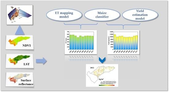
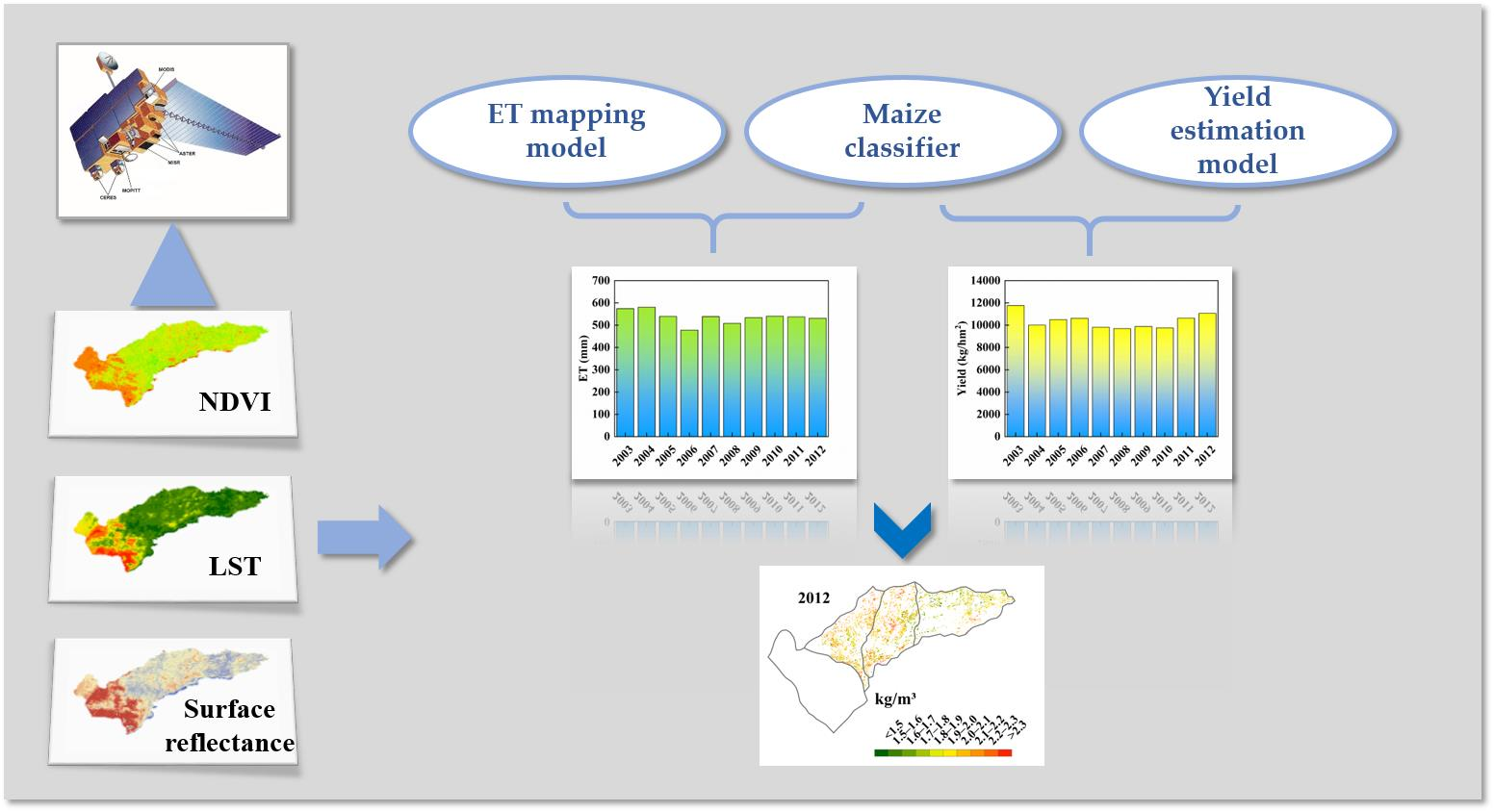
The objective of this study is to assess the WUE of maize in the Hetao Irrigation District in Northwestern China from 2003 to 2012. The 2003 to 2012 period was selected because this was the first decade after the implementation of water-saving rehabilitation in the region (1998–2002). The assessment algorithm includes four main components, including a dual-source model (HTEM) for ET mapping, a classifier for maize mapping based on the ellipsoid state spaces of the vegetation and phenological indices, a crop-yield estimation model based on the crop water production function, and maize WUE assessment based on the above outputs.

2. Materials and Methods

2.1. Study Area

The Hetao Irrigation District (40.0°–41.5°N, 106.0°–109.5°E),located in northwest China, was defined as the study region. The Hetao Irrigation District is a major grain-producing area and the third largest irrigation district in China. Four counties in Hetao, where mainly maize is planted, were selected for the analysis that follows, including Dengkou, Hangjinhouqi, Linhe, and Wuyuan (Figure 1).The study region has a typically arid continental climate, which is characterized by a cold winter with little snowfall and a dry summer with little rainfall. The average annual precipitation is about 150 mm yr⁻¹, and the mean annual temperature is about 6.5 °C [40].

The area of study is mainly plains, with elevations ranging from 1028 m to 1062 m above sea level, except for a small mountainous area in the northwest of Dengkou county. The study region covers a total area of 9308 km², and most of the agricultural lands are concentrated in Linhe, Hangjinhouqi, and Wuyuan counties, whereas desert land and the Gobi Desert cover most parts of Dengkou county. Due to limited precipitation, agriculture in the Hetao Irrigation District mainly depends on irrigation water diverted from the Yellow River along the south boundary of the district.

The crop planting pattern in the study region is complex, with great variations during the period under study. Maize, sunflower, and wheat are three major crops in Hetao. The maize acreage increased from 2003 to 2012 continuously and has become the dominant crop in the region (over 1/3 of the total crop area) since 2012 [41]. Therefore, summer maize was selected as a representative crop, which generally grows from early April to mid-September, with an average growing season length of ~170 days.

2.2. ET Model

The hybrid dual-source scheme and trapezoid framework-based ET model (HTEM) [17] was used to quantify ET in the Hetao Irrigation District from 2003 to 2012. Briefly, HTEM estimates ET based on surface energy balance, which is expressed as

$$R_n=H+\lambda \mathrm{ET}+G$$

(1)

where R_n is net radiation (W/m²) calculated following Allen et al. [14]; H is the sensible heat flux (W/m²), G is soil heat flux (W/m²) (for the detailed calculation processes for G, refer to Long et al. [42]); and λ is the latent heat of evaporation of water (J/kg).

The R_n is then partitioned into radiation received by vegetation canopy and by soil surface,

$$R_{nc}=R_n[1-\exp (-k_c\mathrm{LAI})]$$

(2)

$$R_{ns}=R_n-R_{nc}$$

(3)

where R_nc and R_ns are net radiation of vegetation and soil (W/m²), respectively; LAI and k_c are the leaf area index and the attenuation coefficient of radiation in the canopy, respectively.

For each component (vegetation and soil), the surface energy balance equation can be rewritten as Equations (4) and (5), and sensible heat fluxes of vegetation and soil can be calculated from Equation (6) to Equation (9).

$$R_{nc}={\mathrm{LE}}_c^L+H_c^L$$

(4)

$$R_{ns}={\mathrm{LE}}_s^L+H_s^L+G$$

(5)

$$H_c^P=\rho C_p\frac{T_c-T_a}{r_a^h}$$

(6)

$$H_s^P=\rho C_p\frac{T_s-T_a}{r_a^a+r_a^s}$$

(7)

$$H_c^L=f_c\times H_c^P$$

(8)

$$H_s^L=(1-f_c)\times H_s^P$$

(9)

where superscripts L and P represent layered flux and patch flux, respectively; subscript s and c represent soil and vegetation, respectively; f_c is the vegetation fraction that can be estimated from NDVI [43,44]; $r_a^h$, $r_a^a$, and $r_a^s$ are the aerodynamic resistance (s/m) that can be calculated following Sánchez et al. [45]; T_c and T_s represent the temperatures of vegetation surface and soil surface (°C), respectively; T_a is the air temperature at reference height (°C). The relationship between T_c, T_s and land surface temperature (LST) based on RS data can be described as follows:

$${\mathrm{LST}}^4=f_c\times T_c^4+(1-f_c)\times T_s^4$$

(10)

Estimation of T_s and T_c from LST is the key process in dual-source ET models, and a trapezoid framework of vegetation fraction and land surface temperature is used in HTEM. Then LE_c and LE_s can be calculated from Equations (4) and (5). For a detailed description of HTEM in determining ET, evaporation, and transpiration, refer to [17].

The ET derived from HTEM is an instantaneous value at the satellite overpassing time. To obtain long-term ET information, an appropriate temporal upscaling algorithm should be selected. The crop coefficient (Kc) method was used, which performs best in cropland with ET upscaling from the instantaneous scale to the daily scale, according to Chávez et al. [46]. Due to the satellite revisiting cycle, cloud obscuration, and other factors, RS images were not always available on all days of the crop growing period. For days lacking RS images, Kc could be obtained by linear interpolation between two adjacent days with available RS images [47].

In this study, two methods were used to evaluate the accuracy of HTEM-estimated ET. First, the observed ET in 2009 was used to evaluate the accuracy of the estimated ET at the field scale [48]. For the regional scale, a water balance analysis was conducted to evaluate the performance of HTEM during the growing seasons (April to October) from 2003 to 2012. The water balance equation is written as follows:

$${\mathrm{ET}}_{wb}=P+D-R-\Delta S$$

(11)

where ET_wb is the calculated ET according to the water balance equation (mm); P means total precipitation and D is the total water drawn from the Yellow River; R is the total outflow volume from the study region; the difference between D and R is the net water diversion in the study region; ΔS is the variation of soil water storage in saturated and unsaturated zones in the crop growing season. Root-mean-square error (RMSE) and relative error (RE) were selected to evaluate the accuracy of estimated ET at the regional scale.

2.3. Crop Mapping Algorithm

To map multi-year distributions of maize in a large irrigation district under a complex planting pattern, the crucial task is to capture the characteristics that can distinguish maize from other crops. In this study, a field investigation was carried out to obtain representative sampling points of maize. Then, an asymmetric logistic function was selected to fit the NDVI time series of sampled maize points. By analyzing the characteristics of the logistic curve, the phenological values of maize could be identified. Finally, appropriate phenological values and vegetation indices were chosen to develop a maize classifier.

Specifically, an asymmetric logistic function [49] was used to fit the NDVI time series,

$$\mathrm{NDVI}(t)=a+(b/f){(1+n)}^{-(f+1)/f}n{(f+1)}^{(f+1)/f}$$

(12)

$$n=\exp [(t+d\ln (f)-c)/d]$$

(13)

where NDVI(t) is the NDVI value at DOY of t; and a, b, c, d and f are fitting parameters of the logistic curve. The least-squares method was used in the curve fitting. Two characteristic points can be calculated from Equations (12) and (13), including (i) the maximum value of NDVI and its corresponding time (t_max, NDVI_max) when the first derivative of Equation (12) is equal to 0 and (ii) the left inflection point (t_inf, NDVI_inf), when the second derivation of Equation (12) is equal to 0.

Based on the asymmetric logistic curve, the difference between t_max and t_inf, representing the fast growth period (FGP), was selected as a representative phenological index. Meanwhile, NDVI_inf was selected as a representative vegetation index [50]. Consequently, a maize classifier based on phenology and growth information was established to map the spatial distribution of maize for multiple years over the study region. Based on the sampling points, we found that sampling FGP-NDVI_inf points can be enclosed by an ellipse [50]. The minimum ellipse that encloses all sampled points is calculated by the analytic equation of an ellipse,

$$A{x}^2+Bxy+C{y}^2+Dx+Ey+F=0$$

(14)

where A, B, C, D, E and F are the fitting parameters of the crop classifier; and x and y are the phenological index and the vegetation index, respectively. These fitting parameters can be calculated by minimizing the area of the ellipse encircling all sampled points. Considering that the sampling points of limited number might not contain the entirety of the information about the maize in the Hetao Irrigation District over the studied period, the semi-major and semi-minor axes of the minimum ellipse should be amplified by certain ratios to account for maize growth conditions that were not represented by the sampling points. The total maize planting areas for three years (2010–2012) in the study region were used to determine the amplifying ratios of the semi-major and semi-minor axes, and the maize planting areas of the other seven years (2003–2009) were retained for the evaluation of precision.

By calculating the phenological index and the vegetation index for each pixel according to Equations (12) and (13), the feature point (FGP, NDVI_inf) of each pixel can be obtained. If the feature point falls in the ellipse, the pixel was identified to be maize. Otherwise, it was classified as other crops. For a detailed description of the maize classifier, refer to Jiang et al. [50].

The kappa coefficient [51], which was selected to examine the consistency between the maize classifier and field survey, is as follows:

$$\kappa =\frac{P_o-P_c}{1-P_c}$$

(15)

where P_o and P_c are observed agreement and chance agreement, respectively.

2.4. Estimation of Crop Yield

The Stewart water production function, which describes the relationship between crop ET and yield, was used for crop yield estimation [52],

$$\frac{Y}{Y_m}=1-{\displaystyle \sum _{i=1}^M{\beta }_i\left(1-\frac{{\mathrm{ET}}_i}{{\mathrm{ET}}_{m,i}}\right)}$$

(16)

where Y and Y_m are actual crop yield (kg/hm²) and the maximum crop yield without water stress (kg/hm²), respectively; m is the total days of crop growth; i is the number of days during the crop growth period; ET_i and ET_m,i represent the actual and the maximum crop evapotranspiration of the day i (mm/day), respectively; and β_i is the water sensitivity index that can be calculated by Equations (17) and (18) [53].

$$Z(t)=\frac{K}{1+B{(M/t-1)}^n}$$

(17)

$$\beta (t)=n\frac{Z(t)[1-Z(t)/K]}{t(M-t)}{M}^{2}dt$$

(18)

where Y_m, B, K and n are parameters that can be calibrated by the least squares method with the minimum squared error between the statistical and estimated maize yields as the objective function. The water sensitivity index is close to 0 during the crop sowing and harvesting periods, which are less sensitive to water stress. For a detailed description of the model, refer to Jiang et al. [54].

2.5. Water-Use Efficiency (WUE) Assessment

WUE of maize can be calculated from [55],

$${\mathrm{WUE}}_{\mathrm{ET}}=\frac{Y}{\mathrm{ET}}$$

(19)

$${\mathrm{WUE}}_T=\frac{Y}{T}$$

(20)

where ET and T are the total evapotranspiration and transpiration of maize during the growing season (m³/hm²), respectively, and WUE_ET and WUE_T are maize WUE based on evapotranspiration and transpiration (kg/m³), respectively.

2.6. Data Sources

The Moderate Resolution Imaging Spectroradiometer (MODIS) data were chosen as the main RS data in this study due to their appropriate spatial and temporal resolutions and availability on a global scale from 2000 (https://ladsweb.modaps.eosdis.nasa.gov (accessed on 15 October 2019)). Two specific MODIS datasets (MOD09GA and MOD11A1) were used to obtain the reflectance of specific bands, LST, and other required information. All original RS data were re-projected into the UTM projection and resampled to a 250 m spatial resolution. Images with a cloud cover larger than 5% were not used (

Table A1. MODIS images used in this study.

Year	Total Number	Day of Year
2003	58	36, 43, 54, 57, 68, 79, 80, 85, 103, 105, 108, 110, 114, 120, 121, 128, 129, 139, 144, 148, 153, 156, 157, 164, 173, 174, 189, 201, 208, 214, 217, 223, 228, 231, 235, 245, 251, 253, 255, 256, 265, 266, 274, 287, 288, 290, 294, 297, 299, 303, 306, 308, 319, 326, 333, 335, 340, 347
2004	65	2, 37, 41, 50, 53, 60, 66, 71, 90, 92, 94, 98, 99, 101, 105, 108, 114, 117, 119, 126, 128, 133, 142, 151, 160, 162, 172, 174, 183, 188, 202, 208, 217, 220, 225, 229, 238, 241, 244, 247, 252, 259, 261, 264, 265, 266, 270, 275, 277, 281, 284, 286, 288, 295, 300, 302, 313, 316, 320, 325, 334, 336, 339, 345, 354
2005	61	50, 64, 66, 71, 76, 78, 82, 87, 94, 99, 103, 105, 107, 110, 117, 121, 123, 126, 128, 131, 133, 147, 149, 153, 162, 164, 169, 171, 173, 186, 196, 204, 212, 215, 229, 238, 244, 245, 251, 256, 265, 276, 279, 281, 283, 288, 290, 297, 302, 304, 309, 313, 315, 317, 322, 324, 327, 329, 332, 350, 357
2006	56	8, 49, 54, 60, 65, 67, 72, 74, 79, 81, 83, 85, 88, 105, 110, 113, 120, 126, 133, 138, 142, 147, 151, 154, 161, 165, 167, 177, 181, 186, 207, 209, 211, 213, 218, 227, 232, 245, 248, 252, 259, 277, 282, 284, 289, 291, 294, 295, 298, 303, 305, 309, 312, 314, 318, 325
2007	53	12, 17, 31, 36, 83, 93, 95, 97, 114, 116, 120, 125, 132, 138, 139, 145, 146, 148, 152, 155, 159, 164, 175, 191, 196, 200, 212, 214, 219, 225, 228, 232, 239, 246, 251, 253, 262, 264, 266, 267, 287, 292, 298, 301, 308, 310, 312, 317, 324, 331, 333, 349, 365
2008	64	4, 9, 53, 57, 59, 62, 64, 66, 69, 75, 77, 86, 93, 98, 101, 105, 107, 114, 116, 119, 121, 125, 126, 128, 135, 139, 141, 144, 151, 158, 162, 176, 182, 183, 186, 188, 194, 197, 203, 215, 217, 224, 235, 240, 244, 249, 255, 256, 274, 276, 279, 285, 290, 299, 304, 306, 309, 313, 324, 333, 336, 340, 345, 352
2009	70	22, 27, 32, 36, 41, 45, 50, 59, 64, 72, 79, 82, 87, 91, 95, 98, 105, 111, 116, 119, 123, 125, 132, 137, 142, 146, 150, 151, 155, 164, 171, 174, 175, 176, 180, 182, 187, 192, 196, 205, 212, 214, 217, 221, 223, 224, 225, 226, 228, 231, 239, 242, 244, 254, 260, 264, 265, 267, 269, 271, 275, 279, 281, 285, 287, 290, 297, 299, 301, 311
2010	58	49, 50, 56, 74, 85, 91, 92, 96, 103, 105, 113, 119, 121, 122, 130, 131, 139, 151, 153, 156, 162, 169, 170, 171, 178, 186, 190, 192, 199, 201, 202, 203, 209, 210, 217, 220, 231, 234, 238, 240, 247, 254, 256, 265, 266, 268, 276, 277, 279, 281, 288, 290, 298, 325, 332, 334, 336, 352
2011	55	28, 30, 33, 44, 58, 62, 69, 74, 83, 92, 100, 101, 104, 108, 111, 132, 133, 136, 141, 143, 150, 152, 163, 165, 181, 193, 195, 196, 197, 200, 207, 211, 213, 214, 218, 221, 228, 234, 238, 241, 243, 253, 255, 266, 268, 275, 277, 289, 293, 314, 316, 319, 323, 341, 348
2012	76	32, 34, 38, 41, 45, 49, 52, 57, 66, 68, 70, 72, 83, 84, 90, 95, 97, 107, 112, 118, 122, 130, 135, 137, 139, 143, 145, 151, 153, 160, 162, 164, 167, 168, 169, 177, 184, 186, 187, 193, 205, 208, 211, 221, 222, 225, 232, 234, 235, 239, 241, 242, 248, 250, 257, 258, 263, 271, 272, 273, 276, 283, 285, 296, 299, 301, 303, 305, 306, 317, 319, 324, 330, 331, 333, 344

). The broadband surface albedo and NDVI were calculated using specific MODIS reflectance bands following Liang et al. [56] and Huete et al. [57].

The land use map used in this study was downloaded from the Environmental and Ecological Science Data Center for West China (http://westdc.westgic.ac.cn (accessed on 1 November 2019)). DEM data and meteorological data for the Hetao Irrigation District were downloaded from http://srtm.csi.cgiar.org (accessed on 20 November 2019) and http://data.cma.cn (accessed on 3 December 2019). All data were resampled into a 250 m spatial resolution to be consistent with the MODIS data.

A field investigation on the locations of the maize fields was carried out throughout the study region in 2012. A total of 29 representative maize points were selected based on a global positioning system with positioning accuracy of 2–5m (Figure 1b). Statistical acreage and yield data for the maize used in this study are available at the Bayannur Agricultural Information Network (http://www.bmagri.gov.cn (accessed on 30 December 2019)). Water diversion and drainage data used for water balance analysis were obtained from the Hetao Irrigation District Administration in the Inner Mongolia Autonomous Region (http://www.zghtgq.com (accessed on 10 January 2020)).

3. Results

3.1. Model Validation of HTEM and Spatiotemporal Patterns of ET

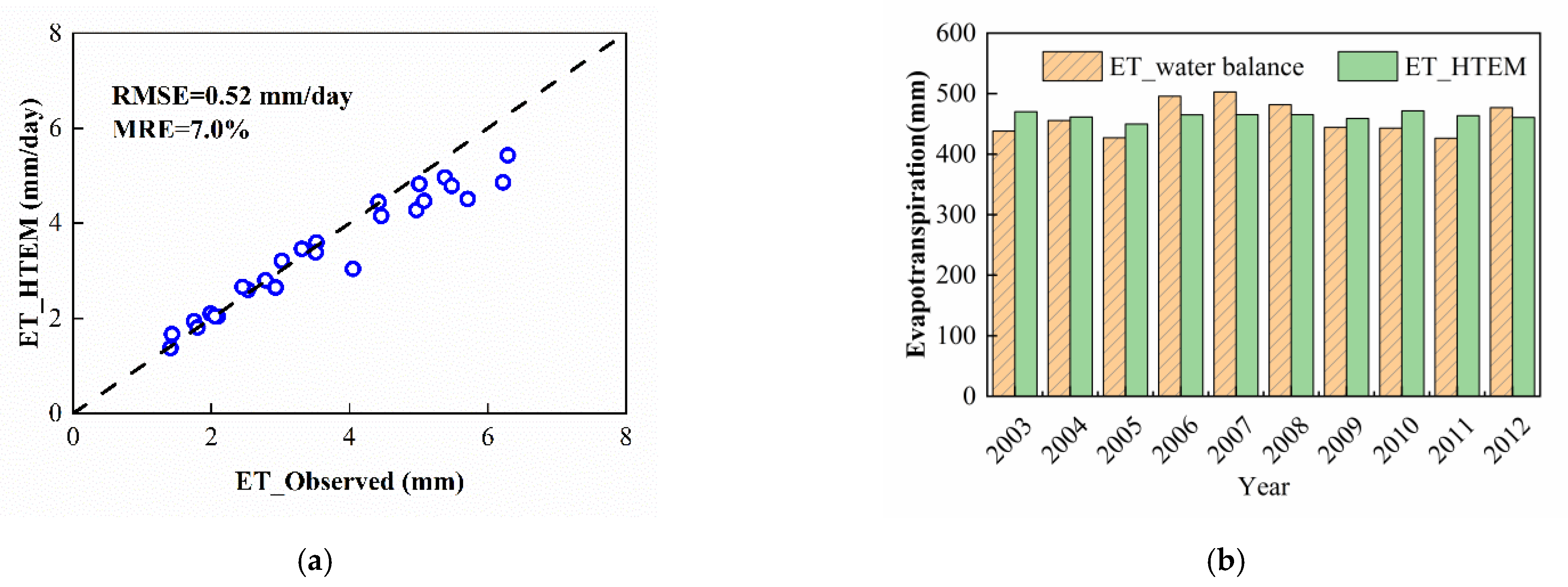
At the field scale, ET estimated by HTEM closely agrees with the observation (Figure 2a), with an RMSE of 0.52 mm/day and a mean relative error of 7.0%. The results also showed that the performance of HTEM in the early and late growth stages was generally better than that in the middle growing season when ET is higher. At the regional scale, The ET during the crop growing season estimated by HTEM agreed well with those estimated by the water balance approach (Figure 2b), with an RMSE and relative error of 26.21 mm/year and 5.3%, respectively.

Evapotranspiration based on RS data not only provides the total water consumption for different land use types but also describes the spatiotemporal variations of ET on a regional scale. Taking the year 2012 as an example, the spatial distribution of plant growing period ET, evaporation (E), and transpiration (T) in the study region is illustrated in Figure 3. Generally, the growing season ET in the northeast of the Hetao Irrigation District is relatively higher (generally higher than 600 mm), whereas that in the southwest is significantly lower (lower than 250 mm). The growing season ET of the study region ranges from 100 mm to 800 mm, and the maximum value occurs in the area near the Yellow River, along the southern edge of the Hetao Irrigation District.

The partitioning of soil evaporation and crop transpiration is an advantage of the dual-source ET models (e.g., HTEM used herein). During the growing season, transpiration ranges from 250 to 350mm in farmland (Figure 3c) and accounts for 48% of ET on average. Desert lands and the Gobi Desert occupy most of the southwest regions, with low vegetation coverage, which leads to smaller transpiration there. Soil evaporation during the growing season ranges from 250 to 350 mm in most farmland (Figure 3b), accounting for 52% of the total ET. The highest evaporation is found in flood plains on the left bank of the Yellow River along the southeast edge of the study area, which is caused by low vegetation coverage and high soil moisture due to river flooding and seepage [58].The total ET, soil evaporation (E) and vegetation transpiration (T) of agricultural land during the growing seasons from 2003 to 2012 are shown in Appendix A (

Table A2. Total ET, soil evaporation (E), and vegetation transpiration (T) of agricultural land during the growing seasons from 2003 to 2012.

Year	2003	2004	2005	2006	2007	2008	2009	2010	2011	2012	Max	Min	Average
ET/mm	625	618	600	599	624	603	617	640	622	617	640	599	617
E/mm	287	317	306	331	310	326	332	335	325	319	335	287	319
T/mm	338	301	294	268	314	277	285	305	297	298	338	277	298
T/ET	0.54	0.48	0.49	0.45	0.50	0.46	0.46	0.48	0.48	0.48	0.54	0.45	0.48

). Our results are broadly consistent with previous findings in the same region. For example, Yang et al. (2012) [20] mapped temporal and spatial patterns of ET in Hetao Irrigation District using the SEBAL model and MODIS data and reported an agricultural land ET ranging from 547 to 605 mm.

3.2. Evaluation of the Crop Classifier and Spatiotemporal Patterns of Maize Distribution

The asymmetric logistic curve described in Equation (12) was chosen to fit the NDVI time series of sampled maize points (Figure 4a). The fitting result showed that the squared correlation coefficient between the fitted and sampled values was as high as 0.99. This result also illustrated that the logistic curve achieved high accuracy in fitting the vegetation index time-series and captured most of the vegetation growth information.

Results of FGP-NDVI_inf at sampled points are illustrated in Figure 4b. The FGP-NDVI_inf points can be approximately encircled by an ellipse. Similar results can also be found in Peña-Barragán et al. [58]. The minimum ellipse that encircled all sampled maize points was calculated by the least squares method (Figure 4b).Based on the total maize planting area for three years (2010–2012) in the study region, the enlarged ratios for the semi-major and semi-minor axes of the minimum ellipse are calibrated to be 1.38 and 1.45, respectively (Figure 4b), and the final ellipse classifier for maize [50] is

$$209x^2+195xy+72y^2-623x-348y+495=0$$

(21)

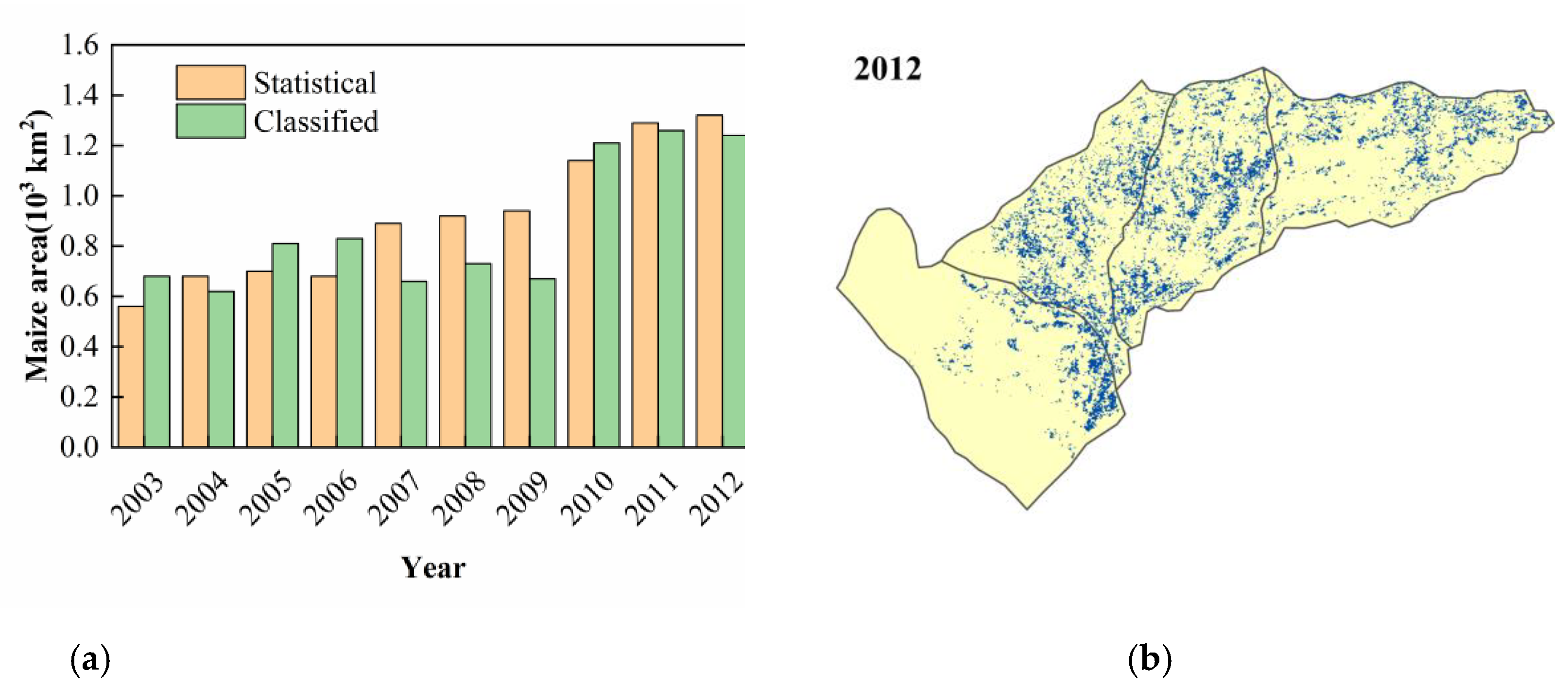
Comparisons of the statistical and classified maize planting areas (Figure 5a) show that the classifier captured most maize land successfully. The average relative error of the classifier for the training years (2010–2012) and testing years (2003–2009) were 5.1% and 20.5%, respectively, and the consistency between the maize classifier and the field investigation was also checked. The kappa coefficient was as high as 0.86, which shows that the mapped maize based on the classifier is consistent with the field investigation.

As an example, Figure 5b shows the spatial distribution of maize in 2012 mapped by the above maize classifier. Little maize is found in Dengkou because most parts are covered with non-agricultural land. On the contrary, Linhe is the most important maize planting region in the study region, and the proportion of maize in all four counties is 32%.

3.3. Maize Evapotranspiration during the Whole Growth Period

Maize ET can be estimated from the results of Section 3.1 and Section 3.2. Due to little maize planting area in Dengkou County, the maize growing season ET of the other three counties (HH, LH and WY) were analyzed and further used in crop yield estimations. Taking Hangjinhouqi as an example, the county-averaged daily ET and T during the maize growing season in 2012 are shown in Figure 6. The results show that maize was sown around the 114th day and harvested around the 278th day, with an average growth period of 165 days. The daily ET during the maize growth period tended to increase first and then decrease, with a total ET of 531 mm. The daily ET at the beginning of the growing season was as small as 2 mm/day and gradually increased thereafter. The daily ET reached the highest value of >5 mm/day around the 200th day. Then the maize ET started to decrease until harvest.

The maize transpiration during the growth period (Figure 6) shows that the total transpiration of maize in Hangjinhouqi was 324 mm in 2012, accounting for 61% of the total ET. The results illustrate that the variation in maize transpiration (T) is generally similar to that of ET. Transpiration of maize is low at the beginning of the growing season when the vegetation fraction is small. Afterward, transpiration increases rapidly. The maximum transpiration of >4 mm/day occurs at about the 200th day and the 220th day. Subsequently, transpiration decreases until the end of the growing season.The detailed ET and T of maize in the study region are summarized in Appendix A (

Table A3. ET and T of maize during the growing seasons from 2003 to 2012.

Year	Hangjinhouqi		Linhe		Wuyuan
	ET/mm	T/mm	ET/mm	T/mm	ET/mm	T/mm
2003	574	373	560	369	594	386
2004	581	361	536	354	568	364
2005	540	343	522	338	497	322
2006	478	305	474	307	486	306
2007	539	356	529	344	523	343
2008	512	310	489	314	479	311
2009	541	310	537	323	533	318
2010	547	353	523	333	512	302
2011	550	352	512	334	544	325
2012	531	324	510	314	553	303
Average	539	339	519	333	529	328

).

3.4. Maize Yield Estimation Based on ET and Maize Mapping

Maize yield over the study region was estimated by the crop water production function, as described in Section 2.4. The simulated result of the crop yield based on the water production function is shown in

Table 1. Results of fitted water production function and accuracy evaluation [54].

Function	Parameters			Accuracy Evaluation
	K	B	n	MRE 1 (%)	MAE 1 (kg/hm2)	R2
Stewart	1.10	2.76	5.00	4.30	446.33	0.75

¹ MRE and MAE refer to mean relative error and mean absolute error, respectively.

[54]. The results show that the estimated yield agrees well with the statistical yield during the study period. The mean relative error and the mean absolute error of the Stewart function are 4.30% and 446.33 kg/hm², respectively, and the correlation coefficient between estimated yield and statistical yield is 0.75. The results of estimated maize yields averaged in three counties from 2003 to 2012 can be found in

Table 2. Comparison of estimated and statistical maize yields in three counties from 2003 to 2012.

Year	Hangjinhouqi			Linhe			Wuyuan
	Estimated Yield (kg/hm2)	Statistical Yield (kg/hm2)	Relative Error (%)	Estimated Yield (kg/hm2)	Statistical Yield (kg/hm2)	Relative Error (%)	Estimated Yield (kg/hm2)	Statistical Yield (kg/hm2)	Relative Error (%)
2003	11,737.06	13,313.34	11.84	11,508.48	11,484.26	0.21	11,998.44	10,479.76	14.49
2004	10,144.89	11,169.42	9.17	9999.46	9917.54	0.83	9970.73	9010.49	10.66
2005	10,322.50	11,184.41	7.71	10,267.22	9932.53	3.37	9722.08	9160.42	6.13
2006	10,466.77	11,154.42	6.16	9988.67	9925.04	0.64	9821.04	9152.92	7.30
2007	9627.42	9992.50	3.65	9177.72	9107.95	0.77	8602.49	8268.37	4.04
2008	9695.19	10,202.40	4.97	9821.48	9767.62	0.55	10,018.23	9580.21	4.57
2009	10,069.08	10,224.89	1.52	10,116.72	10,119.94	0.03	9906.74	9745.13	1.66
2010	9797.02	10,337.33	5.23	10,282.75	10,187.41	0.94	10,306.02	9887.56	4.23
2011	10,710.15	10,277.36	4.21	9550.31	10,082.46	5.28	9947.46	9902.55	0.45
2012	10,956.75	10,682.16	2.57	10,328.28	10,172.41	1.53	10,418.75	10,862.07	4.08
Mean	10,352.68	10,853.82	4.62	10,104.11	10,069.72	0.34	10,071.20	9604.95	4.85

. It is seen that the average annual maize yield estimated in Hangjinhouqi, Linhe and Wuyuan are 10,353 kg/hm², 10,104 kg/hm² and 10,071 kg/hm², respectively. By comparing the maize yields of different counties, Hangjinhouqi and Wuyuan have the highest and lowest maize yields, respectively. The relative errors between estimated yield and statistical yield in Hangjinhouqi, Wuyuan, and Linhe range from 1.52% to 11.84%, from 0.45% to 14.49%, and from 0.03% to 5.28%, respectively. Compared with other similar studies [59,60], the maize yield estimation model based on crop water production function is reliable, with high accuracy.

3.5. Spatiotemporal Variations of Maize WUE from 2003 to 2012

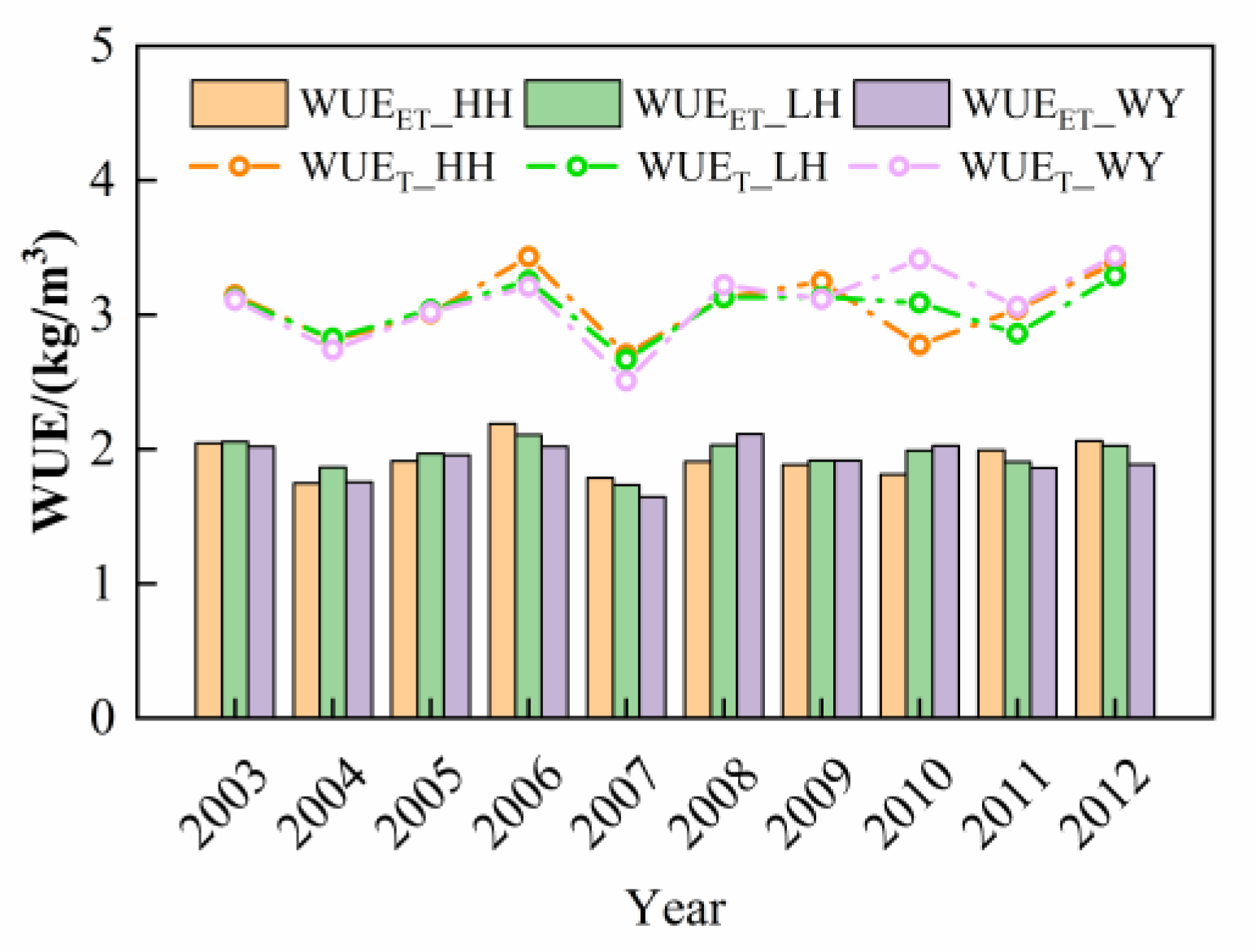
Spatial distributions of WUE_ET and WUE_T in four representative years are shown in Figure 7 and Figure 8, and the annual WUE_ET and WUE_T averaged in the three counties are given in Figure 9. The average annual WUE_ET of maize in Hangjinhouqi (HH), Linhe (LH), and Wuyuan (WY) are 1.93 kg/m³, 1.96 kg/m³, and 1.92 kg/m³, respectively, with little inter-annual variation (Figure 9), and the WUE_ET in Linhe is slightly higher than the other two counties in most years (Figure 7 and Figure 9). Meanwhile, the average annual WUE_T of maize in these three counties varied greatly during the study period (Figure 8 and Figure 9). Wuyuan and Linhe exhibited the highest and lowest average WUE_T of 3.08 kg/m³ and 3.04 kg/m³, respectively. Considering the spatial distribution of WUE_ET, maize planting maybe more concentrated in the middle parts of the study region (e.g., Linhe and Hangjinhouqi).

The WUE_ET and WUE_T varied over the years. Taking Hangjinhouqi as an example, the WUE_ET of maize ranged from 1.75 kg/m³ in 2004 to 2.19 kg/m³ in 2006, with an average value of 1.93 kg/m³ in the study period, while the average annual WUE_T varied more than the WUE_ET, ranging from 2.70 kg/m³ in 2007 to 3.43 kg/m³ in 2006, with an average of 3.07 kg/m³. These results are consistent with the results in [61], which simulated the crop water-use efficiency of Hangjinhouqi in 2012 and 2013 based on the Hydrus-Epic model.

4. Discussion

In this study, we assessed the water-use efficiency (WUE) of maize in three counties of the Hetao Irrigation Districts from RS-based maize mapping and ET and maize yield estimation models. The maize mapping and ET estimation models were fed with MODIS data, and the maize yield estimation model took the estimated ET as input. These models were calibrated and validated with field experiments, field surveys, and/or official statistical data. Results show that the accuracy levels of the models are all satisfactory.

Based on the WUE estimation results, the impact of total water input (precipitation + net water diversion from the Yellow River) on ET, T, yield, and WUE were further analyzed (Figure 10). In the study period, total water input decreased slightly due to the water-saving practices in the Hetao Irrigation District, which caused a slight decrease in maize transpiration and ET (Figure 10a), although the decreasing trends are not statistically significant at the significance level of 0.05. Meanwhile, the maize yield also showed a slight decreasing trend (Figure 10b), but the relative rate of decrease (the ratio of the absolute value of slope to constant in the fitted trend line) was slightly smaller than that of ET and significantly smaller than that of T. As a result, both WUE_ET and WUE_T showed increasing trends, especially WUE_T (Figure 10b). These results imply a negative correlation between WUE and the total water input, and the reduction in total water input may improve WUE to a certain extent, especially for WUE_T. Moreover, these results also demonstrate the effect of the water-saving rehabilitation program, i.e., increased WUE with decreased net water diversion.

Considering the trade-off between maize yield decrease and WUE increase, the water-saving program should be planned properly to avoid a significant decrease in maize yield. The reduced irrigation water diversion from the Yellow River during the study period resulted in a decrease in maize yield, which will become more severe if the amount of irrigation water continues to decrease. Maintaining a relatively steady level irrigation water diversion is necessary for the sustainability of crop production in the region.

5. Conclusions

The growing seasons (April to October) ET and maize cover from 2003 to 2012 in the Hetao Irrigation District were mapped using HTEM and a crop classifier fed with MODIS data. Maize yield was then estimated by the crop water production function, and the WUE of maize was estimated and analyzed for the study period. The results are summarized as follows:

(1)

The HTEM model performs well in the study region, with RMSE of 0.52 mm/day at the field scale and 26.21 mm from April to October at the regional scale during the whole study period.

(2)

The asymmetric logistic function is applicable in describing the maize NDVI time series at sampling points with a mean coefficient of determination of 0.99. Meanwhile, a classifier based on phenological and vegetation indices can obtain spatial distribution and determine the inter-annual variability of maize cover in multiple years. The mean relative errors for the training and testing years were 5.13% and 20.53%, respectively.

(3)

The maize yield estimation model based on the Stewart water production function can estimate maize yield with high accuracy in multiple years. The mean relative error and mean absolute error between estimated yield and statistical yield were 4.30% and 446.33 kg/hm², respectively.

(4)

The average annual WUE_ET and WUE_T in the Hetao Irrigation District were 1.94 kg/m³ and 3.06 kg/m³, respectively. The results show a negative correlation between WUE and net water diversion.

This study provides a reliable method for mapping crop WUE on a regional scale. More studies on WUE in the Hetao Irrigation District in recent years will continue, for example, by mapping more kinds of crops under complex planting structures with high spatiotemporal-resolution remote-sensing data, by analyzing the spatiotemporal variation of WUE in recent years, by identifying the major influencing factors (vapor pressure deficit, CO₂ concentration, temperature, photosynthetic efficiency, etc.), and by understanding the response mechanisms of WUE to climate change and human activity.

References

- Vörösmarty, C.J.; Green, P.; Salisbury, J.; Lammers, R.B. Global water resources: Vulnerability from climate change and population growth. Science 2000, 289, 284–288. [Google Scholar] [CrossRef] [PubMed] [Green Version]
- Godfray, H.C.J.; Beddington, J.R.; Crute, I.R.; Haddad, L.; Lawrence, D.; Muir, J.F.; Pretty, J.; Robinson, S.; Thomas, S.M.; Toulmin, C. Food security: The challenge of feeding 9 billion people. Science 2010, 327, 812–818. [Google Scholar] [CrossRef] [PubMed] [Green Version]
- Chaudhary, S.K.; Srivastava, P.K. Future challenges in agricultural water management. In Agricultural Water Management; Academic Press: Cambridge, MA, USA, 2021; pp. 445–456. [Google Scholar]
- Dregne, H.; Kassas, M.; Rozanov, B. A new assessment of the world status of desertification. Desertif. Control Bull. 1991, 20, 6–18. [Google Scholar]
- Yang, Y.T.; Shang, S.H.; Jiang, L. Remote sensing temporal and spatial patterns of evapotranspiration and the responses to water management in a large irrigation district of North China. Agric. For. Meteorol. 2012, 164, 112–122. [Google Scholar] [CrossRef]
- Shang, S.H.; Mao, X.M. Data envelopment analysis on efficiency evaluation of irrigation-fertilization schemes for winter wheat in North China. In Proceedings of the International Conference on Computer and Computing Technologies in Agriculture, Beijing, China, 18–20October 2008; Springer: Boston, MA, USA, 2009; Volume 1, pp. 39–48. [Google Scholar]
- Jiang, Y.; Xu, X.; Huang, Q.Z.; Huo, Z.L.; Huang, G.H. Assessment of irrigation performance and water productivity in irrigated areas of the middle Heihe River basin using a distributed agro-hydrological model. Agric. Water Manag. 2015, 147, 67–81. [Google Scholar] [CrossRef]
- Zhang, Y.Q.; Kong, D.D.; Gan, R.; Chiew, F.H.S.; McVicar, T.R.; Zhang, Q.; Yang, Y.T. Coupled estimation of 500 m and 8-day resolution global evapotranspiration and gross primary production in 2002–2017. Remote Sens. Environ. 2019, 222, 165–182. [Google Scholar] [CrossRef]
- Han, C.Y.; Zhang, B.Z.; Chen, H.; Wei, Z.; Liu, Y. Spatially distributed crop model based on remote sensing. Agric. Water Manag. 2019, 218, 165–173. [Google Scholar] [CrossRef]
- Chen, J.M.; Liu, J. Evolution of evapotranspiration models using thermal and shortwave remote sensing data. Remote Sens. Environ. 2020, 237, 111594. [Google Scholar] [CrossRef]
- Norman, J.; Kustas, W.; Humes, K. A two-source approach for estimating soil and vegetation energy fluxes in observations of directional radiometric surface temperature. Agric. For. Meteorol. 1995, 77, 263–293. [Google Scholar] [CrossRef]
- Bastiaanssen, W.G.M.; Menenti, M.; Feddes, R.A.; Holtslag, A.A.M. A remote sensing surface energy balance algorithm for land (SEBAL)-1. Frmulation. J. Hydrol. 1998, 213, 198–212. [Google Scholar] [CrossRef]
- Su, Z.B. The surface energy balance system (SEBS) for estimation of turbulent heat fluxes. Hydrol. Earth Syst. Sci. 2002, 6, 85–100. [Google Scholar] [CrossRef]
- Allen, R.G.; Tasumi, M.; Trezza, R. Satellite-based energy balance for mapping evapotranspiration with internalized calibration (METRIC)-model. J. Irrig. Drain. Eng. 2007, 133, 380–394. [Google Scholar] [CrossRef]
- Mu, Q.Z.; Zhao, M.S.; Running, S.W. Improvement to a MODIS global terrestrial evapotranspiration algorithm. Remote Sens. Environ. 2011, 115, 1781–1800. [Google Scholar] [CrossRef]
- Long, D.; Singh, V.P. A two-source trapezoid model for evapotranspiration (TTME) from satellite imagery. Remote Sens. Environ. 2012, 121, 370–388. [Google Scholar] [CrossRef]
- Yang, Y.T.; Shang, S.H. A hybrid dual source scheme and trapezoid framework based evapotranspiration model (HTEM) using satellite images: Algorithm and model test. J. Geophys. Res-Atmos. 2013, 118, 2284–2300. [Google Scholar] [CrossRef]
- Kamali, M.I.; Nazari, R. Determination of maize water requirement using remote sensing data and SEBAL algorithm. Agric. Water Manag. 2018, 209, 197–205. [Google Scholar] [CrossRef]
- Li, Z.L.; Tang, R.L.; Wan, Z.M.; Bi, Y.Y.; Zhou, C.H.; Tang, B.H.; Yan, G.J.; Zhang, X.Y. A reviewer of current methodologies for regional evapotranspiration estimation from remotely sensed data. Sensors 2009, 9, 3801–3853. [Google Scholar] [CrossRef] [PubMed] [Green Version]
- Yang, Y.T.; Long, D.; Guan, H.D.; Liang, W.; Simmons, C.; Batelaan, O. Comparison of three dual-source remote sensing evapotranspiration models during the MUSOEXE-12 campaign: Revisit of model physics. Water Resour. Res. 2015, 51, 3145–3165. [Google Scholar] [CrossRef]
- Ulaby, F.T.; Li, R.Y.; Shanmugan, K.S. Crop classification using airborne radar and landsat data. IEEE Trans. Geosci. Remote Sens. 1982, 1, 42–51. [Google Scholar] [CrossRef] [Green Version]
- Jia, K.; Wu, B.F.; Li, Q.Z. Crop classification using HJ satellite multispectral data in the North China Plain. J. Appl. Remote Sens. 2013, 7, 3576. [Google Scholar] [CrossRef]
- Zhong, L.H.; Gong, P.; Biging, G.S. Efficient corn and soybean mapping with temporal extendability: A multi-year experiment using Landsat imagery. Remote Sens. Environ. 2014, 140, 1–13. [Google Scholar] [CrossRef]
- Yang, S.T.; Gu, L.J.; Li, X.F.; Jiang, T.; Ren, R.Z. Crop classification method based on optimal feature selection and hybrid CNN-RF networks for multi-temporal remote sensing imagery. Remote Sens. 2020, 12, 3119. [Google Scholar] [CrossRef]
- Wardlow, B.D.; Egbert, S.L. Large-area crop mapping using time-series MODIS 250 mNDVI data: An assessment for the U.S. Central Great Plains. Remote Sens. Environ. 2008, 112, 1096–1116. [Google Scholar] [CrossRef]
- Wardlow, B.D.; Egbert, S.L. A comparison of MODIS 250-m EVI and NDVI data for crop mapping: A case study for southwest Kansas. Int. J. Remote Sens. 2010, 31, 805–830. [Google Scholar] [CrossRef]
- Skakun, S.; Franch, B.; Vermote, E.; Roger, J.; Becker-Reshef, I.; Justic, C.; Kussul, N. Early season large-area winter crop mapping using MODIS NDVI data, growing degree days information and a Gaussian mixture model. Remote Sens. Environ. 2017, 195, 244–258. [Google Scholar] [CrossRef]
- Hu, Q.; Sulla-Menashe, D.; Xu, B.D.; Yin, H.; Tang, H.J.; Yang, P.; Wu, W.B. A phenology-based spectral and temporal feature selection method for crop mapping from satellite time series. Int. J. Appl. Earth Obs. Geoinf. 2019, 80, 218–229. [Google Scholar] [CrossRef]
- Idso, S.B.; Jackson, R.D.; Reginato, R.J. Remote sensing for agricultural water management and crop yield prediction. Agric. Water Manag. 1977, 1, 299–310. [Google Scholar] [CrossRef]
- Singh, R.; Semwal, D.P.; Rai, A.; Chhikara, R.S. Small area estimation of crop yield using remote sensing satellite data. Int. J. Remote Sens. 2002, 23, 49–56. [Google Scholar] [CrossRef]
- Zhang, S.; Bai, Y.; Zhang, J.H.; Ali, S. Developing a process-based and remote sensing driven crop yield model for maize (PRYM-Maize) and its validation over the Northeast China Plain. J. Integr. Agric. 2021, 20, 408–423. [Google Scholar] [CrossRef]
- Doraiswamy, P.C.; Hatfield, J.L.; Jackson, T.J.; Akhmedov, B.; Prueger, J.; Stern, A. Crop condition and yield simulations using Landsat and MODIS. Remote Sens. Environ. 2004, 92, 548–559. [Google Scholar] [CrossRef]
- Xin, Q.C.; Gong, P.; Yu, C.Q.; Yu, L.; Broich, M.; Suyker, A.E.; Myneni, R.B. A production efficiency model-based method for satellite estimates of corn and soybean yields in the Midwestern US. Remote Sens. 2013, 5, 5926–5943. [Google Scholar] [CrossRef] [Green Version]
- Mulianga, B.; Bégué, A.; Simoes, M.; Todoroff, P. Forecasting regional sugarcane yield based on time integral and spatial aggregation of MODIS NDVI. Remote Sens. 2013, 5, 2184–2199. [Google Scholar] [CrossRef] [Green Version]
- Sakamoto, T.; Gitelson, A.A.; Arkebauer, T.J. MODIS-based corn grain yield estimation model incorporating crop phenology information. Remote Sens. Environ. 2013, 131, 215–231. [Google Scholar] [CrossRef]
- Monteith, J.L. Solar-radiation and productivity in tropical ecosystems. J. Appl. Ecol. 1972, 9, 747–766. [Google Scholar] [CrossRef] [Green Version]
- Peng, D.L.; Huang, J.F.; Li, C.J.; Liu, L.Y.; Huang, W.J.; Wang, F.M.; Yang, X.H. Modelling paddy rice yield using MODIS data. Agric. For. Meteorol. 2014, 184, 107–116. [Google Scholar] [CrossRef]
- Claverie, M.; Demarez, V.; Duchemin, B.; Hagolle, O.; Ducrot, D.; Marais-Sicre, C.; Dejoux, J.F.; Huc, M.; Keravec, P.; Béziat, P.; et al. Maize and sunflower biomass estimation in southwest France using high spatial and temporal resolution remote sensing data. Remote Sens. Environ. 2012, 124, 844–857. [Google Scholar] [CrossRef]
- Zhang, J.H.; Yao, F.M. MODIS Satellite data coupled with a vegetation process model for mapping maize yield in the Northeast China. In Proceedings of the International Conference on Geo-Informatics in Resource Management and Sustainable Ecosystem, Wuhan, China, 8–10November 2013; Springer: Berlin/Heidelberg, Germany, 2013; Volume 399, pp. 214–222. [Google Scholar]
- Yu, R.H.; Liu, T.X.; Xu, Y.P.; Zhu, C.; Zhang, Q.; Qu, Z.Y.; Liu, X.M.; Li, C.Y. Analysis of salinization dynamics by remote sensing in Hetao Irrigation District of North China. Agric. Water Manag. 2010, 97, 1952–1960. [Google Scholar] [CrossRef]
- Jiang, L. Remote Sensing-Based Evaluation of Irrigation Efficiency and Crop Water Use Efficiency over Irrigation District in Arid Region; Tsinghua University: Beijing, China, 2016. [Google Scholar]
- Long, D.; Singh, V.P. A modified surface energy balance algorithm for land (M-SEBAL) based on a trapezoidal framework. Water Resour. Res. 2012, 48, 72–84. [Google Scholar] [CrossRef]
- Li, F.; Kustas, W.P.; Prueger, J.H.; Neale, C.M.U.; Jackson, T.J. Utility of remote sensing-based two-source energy balance model under low-and high-vegetation cover conditions. J. Hydrometeorol. 2005, 6, 878–891. [Google Scholar] [CrossRef]
- Zhou, X.B.; Guan, H.D.; Xie, H.J.; Wilson, J.L. Analysis and optimization of NDVI definitions and areal fraction models in remote sensing of vegetation. Int. J. Remote Sens. 2009, 30, 721–751. [Google Scholar] [CrossRef]
- Sánchez, J.M.; Kustas, W.P.; Caselles, V.; Anderson, M.C. Modeling surface energy fluxes over maize using a two-source patch model and radiometric soil and canopy temperature observations. Remote Sens. Environ. 2008, 112, 1130–1143. [Google Scholar] [CrossRef]
- Chávez, J.L.; Neale, C.M.U.; Prueger, J.H.; Kustas, W.P. Daily evapotranspiration estimates from extrapolating instantaneous airborne remote sensing ET values. Irrig. Sci. 2008, 27, 67–81. [Google Scholar] [CrossRef]
- Bastiaanssen, W.G.M.; Ahmad, M.U.D.; Chemin, Y. Satellite surveillance of evaporative depletion across the Indus Basin. Water Resour. Res. 2002, 38, 9-1–9-9. [Google Scholar] [CrossRef]
- Dai, J.X.; Shi, H.B.; Tian, D.L.; Xia, Y.H.; Li, M.H. Determination of crop coefficients of main grain and oil crops in Inner Mongolia Hetao irrigation area. J. Irrig. Drain. 2011, 30, 23–27. (In Chinese) [Google Scholar]
- Royo, C.; Aparicio, N.; Blanco, R.; Villegas, D. Leaf and green area development of durum wheat genotypes grown under Mediterranean conditions. Eur. J. Agron. 2004, 20, 419–430. [Google Scholar] [CrossRef]
- Jiang, L.; Shang, S.H.; Yang, Y.T.; Guan, H.D. Mapping interannual variability of maize cover in a large irrigation district using a vegetation index-phenological index classifier. Comput. Electron. Agric. 2016, 123, 351–361. [Google Scholar] [CrossRef]
- Cohen, J. A Coefficient of agreement for nominal scales. Educ. Psychol. Meas. 1960, 20, 37–46. [Google Scholar] [CrossRef]
- Peng, Z.G.; Liu, Y.; Xu, D.; Wang, L.; Lei, B.; Du, L.J. Estimation of regional water product function for winter wheat using remote sensing and GIS. Trans. Chin. Soc. Agric. Mach. 2014, 45, 167–171. (In Chinese) [Google Scholar]
- Wang, Y.R.; Lei, Z.D.; Yang, S.X. Cumulative function of sensitive index for winter wheat. J. Hydraul. Eng. 1997, 5, 28–34. (In Chinese) [Google Scholar]
- Jiang, L.; Shang, S.H.; Yang, Y.T.; Wang, Y.R. Method of regional crop yield estimation based on remote sensing evapotranspiration model. Trans. Chin. Soc. Agric. Eng. 2019, 35, 90–97. (In Chinese) [Google Scholar]
- Yu, G.R.; Wang, Q.F.; Zhuang, J. Modeling the water use efficiency of soybean and maize plants under environmental stresses: Application of a synthetic model of photosynthesis-transpiration. J. Plant Physiol. 2004, 16, 303–318. [Google Scholar] [CrossRef] [PubMed] [Green Version]
- Liang, S.L. Narrowband to broadband conversions of land surface albedo I Algorithms. Remote Sens. Environ. 2001, 76, 213–238. [Google Scholar] [CrossRef]
- Huete, A.; Didan, K.; Miura, T.; Rodriguez, E.P.; Gao, X.; Ferreira, L.G. Overview of the radiometric and biophysical performance of the MODIS vegetation indices. Remote Sens. Environ. 2002, 83, 195–213. [Google Scholar] [CrossRef]
- Peña-Barragán, J.M.; Ngugi, M.K.; Plant, R.E.; Six, J. Object-based crop identification using multiple vegetation indices, textural features and crop phenology. Remote Sens. Environ. 2011, 115, 1301–1316. [Google Scholar] [CrossRef]
- Su, T.; Feng, S.Y.; Xu, Y. Spring maize yield estimation based on radiation use efficiency and multi-temporal remotely sensed data. Remote Sens. Technol. Appl. 2013, 28, 824–830. (In Chinese) [Google Scholar]
- Yu, B.; Shang, S.H. Multi-year mapping of major crop yields in an irrigation district from high spatial and temporal resolution vegetation index. Sensors 2018, 18, 3787–3801. [Google Scholar] [CrossRef] [PubMed] [Green Version]
- Hao, Y.Y. Simulation of Irrigated Hydrological Processes and Assessment of Water Productivity in Inner Mongolia Hetao Irrigation District; China Agricultural University: Beijing, China, 2015. [Google Scholar]
Figure 1.
Location of the study region (a), location of maize sampling points (b),and land cover classification in the study region as of 2000 (c).
Figure 2.
Comparisons of ET estimated from HTEM with observed ET at field scale (a) and regional ET estimated from water balance analysis (b).
Figure 3.
Spatial distributions of HTEM estimated total ET (a), E (b), and T (c) during the growing season (April to October) in 2012.
Figure 4.
Mean NDVI series for sampled points and fitted asymmetric logistic function in 2012 (a) and the developed ellipse classifier (b).
Figure 5.
Comparisons of statistical and classified maize planting areas from 2003 to 2012 (a) and spatial distribution of maize in 2012 (b).
Figure 6.
Variations in maize ET and T in Hangjinhouqi during the growing season of 2012.
Figure 7.
Spatial distributions of maize WUEET from 2003 to 2012.
Figure 8.
Spatial distributions of maize WUET from 2003 to 2012.
Figure 9.
Average WUE of maize in three counties during the study period.
Figure 10.
Variations in maize evapotranspiration (ET), transpiration (T), and total water input (precipitation + net water diversion, P+Wn) (a) and maize yield, WUEET, and WUET (b) in the study period.