Accessing the Time-Series Two-Dimensional Displacements around a Reservoir Using Multi-Orbit SAR Datasets: A Case Study of Xiluodu Hydropower Station

Abstract

The construction of large-scale hydropower stations could solve the problem of China’s power and energy shortages. However, the construction of hydropower stations requires reservoir water storage. Artificially raising the water level by several tens of meters or even hundreds of meters will undoubtedly change the hydrogeological conditions of an area, which will lead to surface deformation near the reservoir. In this paper, we first used SBAS-InSAR technology to monitor the surface deformation near the Xiluodu reservoir area for various data and analyzed the surface deformation of the Xiluodu reservoir area from 2014 to 2019. By using the 12 ALOS2 ascending data, the 100 Sentinel-1 ascending data, and the 97 Sentinel-1 descending data, the horizontal and vertical deformations of the Xiluodu reservoir area were obtained. We found that the Xiluodu reservoir area is mainly deformed along the vertical shore, with a maximum deformation rate of 250 mm/a, accompanied by vertical deformation, and the maximum deformation rate is 60 mm/a. Furthermore, by analyzing the relationship between the horizontal deformation sequence, the vertical deformation sequence, and the impoundment, we found the following: (1) Since the commencement of Xiluodu water storage, the vertical shore direction displacement has continued to increase, indicating that the deformation caused by the water storage is not due to the elastic displacement caused by the load, but by irreversible shaping displacement. According to its development trend, we speculate that the vertical shore direction displacement will continue to increase until it eventually stabilizes; (2) Vertical displacement increases rapidly in the initial stage of water storage; after two water-storage cycles, absolute settlement begins to slow down in the vertical direction, but its deformation still changes with the change in the storage period.

1. Introduction

As a clean and recyclable resource, hydroelectricity is receiving increasing attention from all countries [1]. Inevitably, the rapid development of China’s economy has led to a huge demand for energy. Southwest China has abundant water resources for the construction of hydropower stations, so it has obtained a reputation as the “Asian battery” [2]. However, the impounding of a reservoir changes the conditions of local hydrogeology and the regional gravity field, resulting in ground deformation [3]. Furthermore, fluctuations in water level accelerate the deformation, causing local geohazards. In 1961, a landslide with a volume of about 165 × 10⁴ ${\mathrm{m}}^3$ occurred in the Zixi Reservoir in Zishui, Hunan Province, causing 40 deaths [4]. In 1963, a landslide occurred in the Vajont Reservoir in Italy; a huge volume of landslide soil (about 270 × 10⁶ ${\mathrm{m}}^3$) rushed into the reservoir, and the surge caused 1925 deaths [5].

The Three Gorges Dam is the largest hydropower station in the world. After the water level of the Three Gorges Dam reached 175 m in 2008, the number of resurrection landslides was tens of times the number from 1992 to 1995 [6]. In order to decrease such geological disasters, scholars are paying more attention to the ground deformation around hydropower stations.

Currently, the tools to monitor ground deformation include the spirit leveling method [7], the Global Positioning System (GPS) [8], and optical remote sensing [9]. However, the spirit leveling and GPS methods are costly and a have low spatial resolution for capturing the detail of a whole deformation pattern [10]. Optical remote sensing is susceptible to the air conditions of clouds and rain.

Synthetic aperture radar interferometry (InSAR), a satellite-based geodetic technique, can overcome the influence of cloud and rain on optical remote sensing and can work both day and night, demonstrating advantages in ground-deformation monitoring [11]. InSAR has been used in the geohazard monitoring of landslides [12], earthquakes [13], volcanos [14], and ground subsidence [15], among others. Additionally, in order to bypass the effects of decorrelation [16] and atmospheric delay [17], scholars have proposed time-series InSAR techniques, such as Persistent Scatterer InSAR (PS-InSAR) [18] and Short Baseline Subset InSAR (SBAS-InSAR) [19]. The PS-InSAR or SBAS-InSAR techniques can recover long-temporal time-series ground deformations with accuracy levels of mm to cm. Recently, scholars have applied time-series InSAR to monitor the landslide at hydropower stations, such as the Three Gorges Dam [10] and the Wudongde Hydropower Station [20].

The Xiluodu Hydropower Station is located upstream of the Jinsha River in China. As the world’s third-largest hydropower station, the Xiluodu Hydropower Station has experienced frequent landslides and other geohazards since its impoundment in 2013. In 2013, the Huangping landslide, with an inflow of earthworks amounting to 20 × 104 ${\mathrm{m}}^3$, caused 12 deaths. The Ganhaizi landslide, with an influx of earthworks of 7800 × 104 ${\mathrm{m}}^3$, was the largest landslide that occurred at the Xiluodu Hydropower Station [21]. LIANG Guohe [22] and ZHOU Zhifang [23] used the leveling points and valley-shrink surveying lines, respectively, to monitor subsidence and valley-shrink deformation around the shoreside of the Xiluodu reservoir and the Xiluodu arch dam, and their results showed that the Xiluodu arch dam and the shoreside of the reservoir were under valley-shrinkage deformation of 50 mm, accompanied by about 25 mm subsidence. Additionally, ZHOU Zhifang [23] pointed out that valley-shrinkage deformation is highly correlated with the water level. In 2017, LI Lingjing [24] analyzed the Yizicun landslide with ALOS, ASAR, and TerraSAR datasets and found that there was a push-type landslide before the water impoundment and that the landslide changed to a pull-type after the water impoundment.

Currently, the research on the Xiluodu Hydropower Station has focused on valley-shrinkage deformation of the shoreside and the arch dam and their subsidence. In 2019, Li et al. [25] used D-InSAR technology to determine the vertical and horizontal displacement of the landslide near the Xiluodu Hydropower Station and further analyzed its deformation characteristics. In 2022, Zhu et al. [26] obtained the horizontal and vertical displacement of the landslide of the Xiluodu Water Station by SBAS technology, using ALOS2 ascending and descending data, and explained the cause of slope instability by combining geomorphic data and lithologic characteristics.

However, these studies were mainly based on traditional measurements and could not completely reflect the ground deformations occurring near Xiluodu. Although the InSAR technique was used to monitor the Xiluodu reservoir area, it was limited to a specific landslide. Furthermore, the hydrogeological conditions have changed after water impoundment. Whether the change in the hydrogeological conditions will lead to wide-range deformation in Yongshan and Leibo counties and change the relationship between the water level and deformation, needs to be analyzed.

2. Geological Setting

2.1. Geological Setting of Xiluodu

As the backbone project of “Power Transmission from West to East” in China, Xiluodu is the largest hydropower station on the Jinsha River. The Xiluodu Hydropower Station is located in the U-shaped river valley upstream of the Jinsha River. On its left side is Leibo County of Sichuan Province, and on its right side is Yongshan County of Yunnan Province. The construction of Xiluodu Hydropower Station started in April 2007, and Xiluodu Hydropower Station carried out the first stage of water storage trial operation in May 2013. In June 2014, Xiluodu Hydropower Station officially began operating, and at the end of September, the water level of the reservoir reached 600 m for the first time. The Xiluodu Hydropower Station is mainly designed to generate power, control floods, fix sand, and navigation [27].

As shown in Figure 1, the reservoir area is located on the southwestern margin of the Yangtze platform, which is the transitional zone between the Yunnan–Guizhou Plateau and the Sichuan Basin. The terrain is generally high in the west and low in the east, belonging to the strong erosion of the high-mountain landform [28]. The Xiluodu Hydropower Station is located at the junction of the first and second steps of China. Rapid changes in the terrain may easily cause geological disasters. Moreover, with the completion of the hydropower station, significant fluctuations in water levels will significantly affect the fragile geological environment.

As shown in Figure 2, the Xiluodu area is surrounded by the yellow mud slope anticline in the north, the wall rock syncline in the south, the Majinzi fault (F1) in the west, and the Jiziba fault (F2) in the east, forming a relatively stable zone. However, a thrust—nappe structure fault (named Majiahe, F3) is located 3 km from the dam area, and the number of thrust outliers is influenced by the Majiahe fault. When the water level of the Xiluodu reservoir increases, most of the thrust outliers are submerged, and subsequently, the fault becomes unstable, affecting the safety of the dam area [29].

2.2. Impoundment of Xiluodu

As shown in Figure 3a, the water level reached its highest level of 600 m in October 2014 for the first time. The water level dropped to 590 m in March 2015. In June 2015, the water level rapidly dropped to 540 m, and then a new round of water storage was started. In July 2015, the water level rose to 555 m. In August 2015, the water level rose to 560 m. In October 2015, it reached 600 m again. Since the water impoundment in October 2014, four complete water impoundment cycles have been completed. Because the annual rainfall is different, the water storage mode is adjusted accordingly.

The distribution of the Xiluodu aquifers changed significantly after water impoundment. The geological setting mainly comprises three water-repellent layers (i.e., S, P2βn, and P2x) and three water-permeable layers (i.e., P1 m, P2β, and Q) [23]; see Figure 3b. The highest water level is 600 m, which is lower than the elevation of the sandy shale layer (P2x). Therefore, only the P1 m and P2β permeable bed layers are directly connected with the reservoir water during the process of impoundment. The potential energy of Xiluodu water increases with the water level. For the P1 m limestone permeable bed layers in a pressurized state, the water permeates the P1 m layer through the exposed limestone area, increasing the P1 m pressure potential energy. For the P2β basalt permeable bed layers in a state of low pressure, the water will directly flow into the P2β layer through the submerged basalt area (see the green arrow in Figure 3b), causing the P2β layer to be saturated gradually.

When the water level rises to 600 m, the rising value of the water level (the difference in L2 and L1) is about 220 m. It leads to an increase in the water’s potential energy. Due to the existence of confining beds (Rammell layer P2βn), the groundwater pressure potential energy under P2βn will generate an oblique upward pressure (see the solid red arrow in Figure 3b), which will cause the uplift and horizontal displacement perpendicular to the shoreline (see the red dash arrow in Figure 3b). Moreover, as the P2β layer becomes increasingly saturated, the saturated soil will consolidate under the action of gravity, causing vertical subsidence.

3. Methods

3.1. Theoretical Basis of Two-Dimensional Deformation Decomposition

The InSAR measures a one-dimensional deformation along the line of sight (LOS) direction, and such measurements can lead to misinterpretation, as the true deformations may consist of horizontal and vertical displacements [30]. As is known, the LOS deformation is the sum of projection results of horizontal (including north–south and east–west components) and vertical displacement in the LOS direction. Given that there are three or more LOS measurements from different viewing geometries, we can decompose the LOS measurements into north–south, east–west, and vertical displacements by least-squares adjustment [31]. However, for this specific study, we know that displacement along a certain direction is zero or can be ignored based on certain assumptions. For the Xiluodu Reservoir, which is a valley reservoir, the displacement along the direction parallel to the shoreline can be ignored. Thus, the horizontal displacement in a direction perpendicular to the shoreline and the displacement in a vertical direction are sufficient for interpretation. Moreover, due to the small number of viewing angles in the study area, it lacks any redundant observation for us to check for errors if we decomposed the three-dimensional deformations. Thus, we proposed an approach to decompose the InSAR measurements in the LOS direction into two-dimensional displacements, i.e., the horizontal displacement in a direction perpendicular to the shoreline and the vertical displacement.

The specific geometry for decomposing LOS deformation into two-dimensional displacements is shown in Figure 4.

The LOS deformation measurement can be expressed as

$$d_{los}=d_{u}cos\theta +d_{p}cos(\delta -\phi )sin\theta$$

(1)

where $\delta$ is the azimuth angle of a predefined direction, i.e., the clockwise angle with respect to the north direction; $\theta$ is the incident angle of the radar; $\phi$ is the heading angle of the satellite; $h$ and $u$ are the horizontal deformation along predefined direction and vertical deformation, respectively; and $d_{los}$ is the InSAR measured deformation in the LOS direction.

Given that there are $K (K>=2)$ LOS measurements for some specific time periods, there is a set of observation equations written in matrix form:

$$\left[\begin{array}{c}{d}_{los1}\\ d_{los2}\\ ⋮\\ d_{losK}\end{array}\right]=\left[\begin{array}{cc}cos(\delta -{\phi }_1)sin{\theta }_1& cos{\theta }_1\\ cos(\delta -{\phi }_2)sin{\theta }_2& cos{\theta }_2\\ ⋮& ⋮\\ cos(\delta -{\phi }_K)sin{\theta }_K& cos{\theta }_K\end{array}\right]\times \left[\begin{array}{c}h\\ u\end{array}\right]$$

(2)

$$Ax=b$$

(3)

where $A$ is the design matrix with a size of $K\times 2$, $x$ is the unknown parameter vector, and b is the observation vector.

When solving Formula (3), because there are random errors in the interferogram, such as noise and some unremoved clean atmospheric delay phase, a random model needs to be added to constrain some of the errors. In this paper, interferogram coherence is used for weighting; then, we can obtain the two-dimensional deformations by using the least-squares adjustment method:

$$x={(A^{T}PA)}^{-1}{A}^{T}Pb$$

(4)

where $P$ is the weight matrix composed of interferogram coherence.

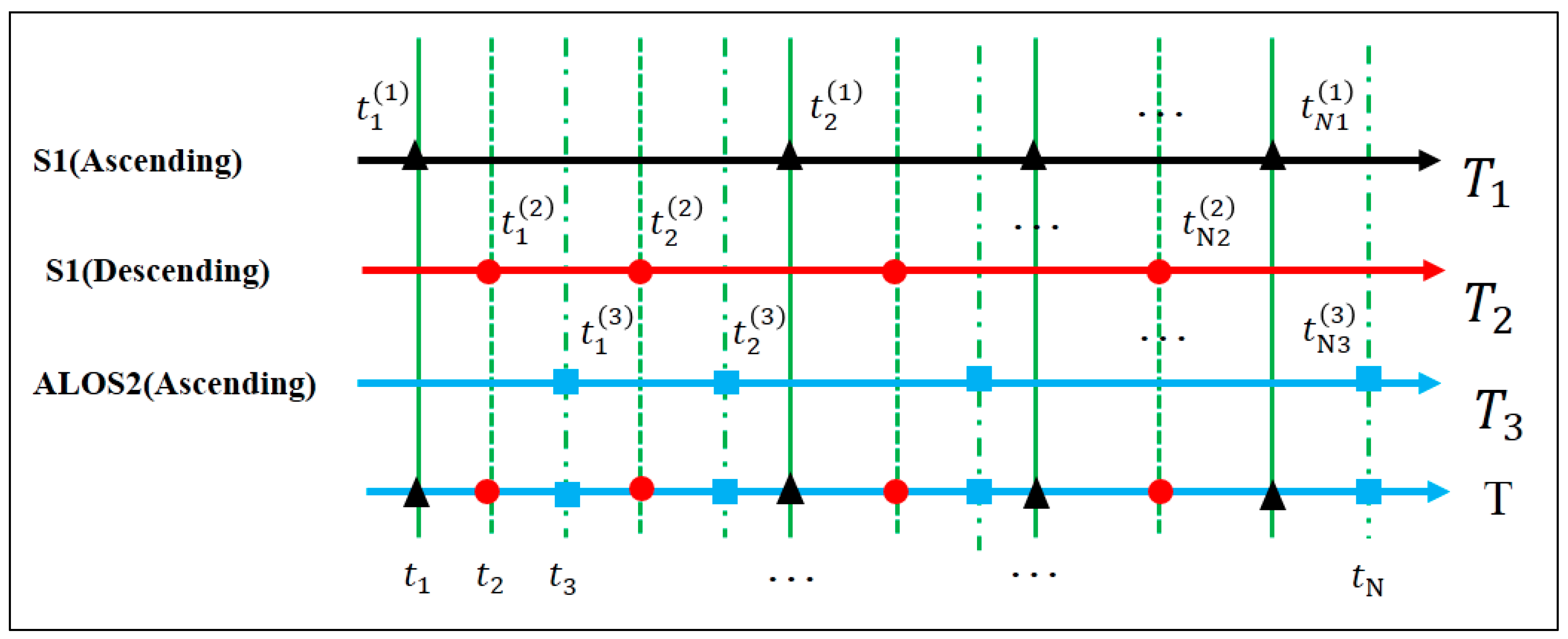
3.2. InSAR Two-Dimensional Deformation Method

Recently, the decomposition of three-dimensional deformation sequences has been developed. Samsonov and D’Oreye proposed the MSBAS method to decompose the time-series East–West and vertical deformations [32] by ignoring the North–South deformations; Pepe et al. proposed the minimum-acceleration (MinA) method, which is used to recover three-dimensional (3D) time-series deformations [33]; Xuguo Shi et al. recovered three-dimensional deformation sequences by using cubic spline interpolation [34]. However, rather than obtaining the 3D deformations or the East–West and vertical deformations by ignoring the North–South deformations, we obtained the vertical and horizontal deformation, called two-dimensional (2D) deformations hereinafter, along a specified direction in reality, which benefits the interpretation.

As shown in Figure 5, given that we have three tracks of SAR data, that is, the Sentinel-1 ascending and descending and ALOS2, covering the study area. The SAR datasets are processed to obtain the time-series LOS deformations. The deformations are geocoded into a geographic coordinate system and further resampled to a common geographic grid. Assuming that the number of images of the three tracks SAR data is $N_1$, $N_2$, and $N_3$, and the acquisition times are $T_1=\left[t_1^{\left(1\right)},t_2^{\left(1\right)},\dots ,t_{N_1}^{\left(1\right)}\right]$, $T_2=\left[t_1^{\left(2\right)},t_2^{\left(2\right)},\dots ,t_{N_2}^{\left(2\right)}\right]$, and $T_3=\left[t_1^{\left(3\right)},t_2^{\left(3\right)},\dots ,t_{N_3}^{\left(3\right)}\right]$, respectively.

Assuming that the acquisition times are unique for different pieces of SAR data, the total number of images is $N=N_1+N_2+N_3$. The times of all of the data acquisitions are $T=T_1\cup T_2\cup T_3$. The corresponding LOS time-series deformations sequence are $d_1=\left[d_1^{\left(1\right)},d_2^{\left(1\right)},\dots ,d_{N_1}^{\left(1\right)}\right]$, $d_2=\left[d_1^{\left(2\right)},d_2^{\left(2\right)},\dots ,d_{N_2}^{\left(2\right)}\right],$ and $d_3=\left[d_1^{\left(3\right)},d_2^{\left(3\right)},\dots ,d_{N_3}^{\left(3\right)}\right]$; then, the merged LOS time-series deformations are $d=d_1\cup d_2\cup d_3$.

According to Equation (2), the LOS time-series deformations d can be written as a set of equations with respect to the time-series 2-D deformations, and expressed in matrix form:

$$Gx=d$$

(5)

where $d={\left[\begin{array}{cccc}{d}_1& d_2& \cdots & d_N\end{array}\right]}^T$ is the observation vector, and the unknown parameters vector $x={\left[\begin{array}{ccccccc}{h}_1& u_1& h_2& u_2& \cdots & h_N& u_N\end{array}\right]}^T$ with a size of $2N\times 1$. The design matrix has a size of $N$ × 2$N$, and its form is as follows:

$$G=\left[\begin{array}{ccccc}{A}_1& & & & \\ & A_2& & & \\ & & A_3& & \\ & & & \ddots & \\ & & & & A_N\end{array}\right]$$

where $A_1=\left[cos(\delta -{\phi }^{\left(1\right)})sin{\theta }^{\left(1\right)}cos{\theta }^{\left(1\right)}\right]$, $A_2=\left[cos(\delta -{\phi }^{\left(2\right)})sin{\theta }^{\left(2\right)}cos{\theta }^{\left(2\right)}\right]$, and $A_3=\left[cos(\delta -{\phi }^{\left(3\right)})sin{\theta }^{\left(3\right)}cos{\theta }^{\left(3\right)}\right]$. The superscript in the angles of $\phi$ and $\theta$ is dependent on which subset of $d_i$ it is from.

Obviously, Equation (5) is rank deficient as the number of equations is smaller than the number of parameters to be estimated, i.e., $N<2N$. To solve the problem of rank deficiency, we add smoothing constraints to the parameters by assuming that the deformation rates of adjacent displacements are equal, i.e.,

$$\frac{h_{i+2}-h_{i+1}}{t_{i+2}-t_{i+1}}=\frac{h_{i+1}-h_i}{t_{i+1}-t_i}$$

(6)

$$\frac{u_{i+2}-u_{i+1}}{t_{i+2}-t_{i+1}}=\frac{u_{i+1}-u_i}{t_{i+1}-t_i}$$

(7)

where $i\in \left[1,N-2\right]$. Then, we obtain a set of equations with respect to unknown parameters vector, and it is expressed by

$$Rx=0$$

(8)

where $R$ is the roughness matrix with a size of $\left(N-2\right)\times N$, and

$$R=\left(\begin{array}{cccccccccccc}{t}_3-t_2& 0& t_1-t_3& 0& t_2-t_1& 0& \dots & \dots & \dots & \dots & 0& 0\\ 0& t_3-t_2& 0& t_1-t_3& 0& t_2-t_1& \dots & \dots & \dots & \dots & 0& 0\\ \dots & \dots & \dots & \dots & \dots & \dots & \dots & \dots & \dots & \dots & \dots & \dots \\ 0& 0& 0& 0& 0& \dots & t_N-t_{N-1}& 0& t_{N-2}-t_N& 0& t_{N-1}-t_{N-2}& 0\\ 0& 0& 0& 0& 0& \dots & 0& t_N-t_{N-1}& 0& t_{N-2}-t_N& 0& t_{N-1}-t_{N-2}\end{array}\right).$$

Combining Equations (5) and (8), we solve the regularized least-squares problem [35]:

$$min\Vert \left[\begin{array}{c}G\\ \alpha R\end{array}\right]x-{\left[\begin{array}{c}d\\ 0\end{array}\right]\Vert }_2^2$$

(9)

The Tikhonov regularization solution is determined by

$$x={(G^{T}G+{\alpha }^2{R}^{T}R)}^{-1}{G}^{T}d$$

(10)

where $\alpha$ is the smoothing parameter and is unknown beforehand. We determine it by using the L-curve method [35].

Figure 6 presents a flowchart of the proposed method.

4. Data Processing and Results

4.1. SAR Data Used

In order to study surface deformation near the Xiluodu reservoir area, we used the ascending and descending data of Sentinel-1 and the ascending data of ALOS2: from October 2014 to March 2019, there was a total of 100 ascending Sentinel-1 data, and the incident angle of the image center was 39.29°. From October 2014 to April 2019, there were 97 descending Sentinel-1 data, and the image center incident angle was 33.9°. From September 2014 to December 2018, there was a total of 12 pieces of ascending ALOS2 data, and the image center incident angle was 31.4°; the coverage area is shown in Figure 7. See

Table 1. Three kinds of data for SBAS interference pair information.

Data	Orbit Type	Track	No. of Images	No. of Int. Pairs	Time Span
S1 A	Ascending	T128	100	197	October 2014–March 2019
S1 A	Descending	T62	97	191	October 2014–April 2019
ALOS2	Ascending	T146	12	21	September 2014–December 2018

for specific information. At the same time, we chose the Shuttle Radar Topography Mission (SRTM) with a 30 m x 30 m resolution to remove the terrain phase.

4.2. Data Processing

We first performed SBAS processing on each piece of data to obtain the deformation sequence of Sentinel-1 data and ALOS2 data. In the data-processing phase, first, in order to ensure the consistency of the three sets of data results, we performed 8 × 2 multi-look on the Sentinel-1 data and 3 × 7 multi-look on the ALOS2 data, thus obtaining image results of about 15 m resolution. Second, because the Sentinel-1 data and ALOS2 data orbital control were accurate, the spatial baseline was short, so the influence of spatial decoherence was not considered. At the same time, in order to overcome the time decoherence, we adopted the two-connected interference pairing method (as shown in Figure 8: 1 and 2 constitute the interference pair, 1 and 3 constitute the interference pair, 2 and 3 constitute the interference pair, and so on), so that any scene image was in a triangular closed loop, which overcame the time decoherence and could test for errors. Therefore, we obtained 21 interference pairs from the ALOS2 ascending data, 197 interference pairs from the Sentinel-1 ascending data obtained, and 191 interference pairs from the Sentinel-1 descending data. Third, we used the SRTM data of 30 × 30 m resolution to obtain the DEM in the SAR coordinate system by geocoding, thus obtaining the simulated terrain phase, and then using the generated interferogram subtracts in the simulated interference phase to remove the terrain phase. In order to eliminate the phase residual and improve the signal-to-noise ratio of the interferogram, we used a ‘Goldstein’ filter on the differential interference phase with a filter factor of 0.5 and a filter window size of 64. As the low-coherence region could be affected by phase noise, we averaged the coherence coefficient map when unwrapping and then ensured that the region with coherence below 0.52 did not participate in the unwrapping, thus ensuring the reliability of the wrap. In the phase unwrapping stage, we selected the unwrapping reference point in the stable region away from the city. After unwrapping with the minimum cost flow, we refined the baseline of the distracted differential interferogram, thereby effectively removing the track phase. Through the above process, we obtained the exact differential interference phase after unwrapping and then converted it into a settlement sequence result. Finally, we inversely geocoded the resulting sedimentation results and resampled them to the same geographic coordinate range to obtain the deformation sequence results for the three images at 15 m resolution.

On this basis, using the algorithm described in Section 3.2, the deformation sequence was decomposed to obtain the deformation sequence results in the vertical shore direction and the vertical direction, and the deformation rate in the horizontal direction and the vertical direction was calculated by using the two-dimensional deformation sequence. The results are provided in Section 4.3.

4.3. Results

4.3.1. LOS Deformation

Figure 9 shows the average rate map of the Sentinel-1 data and ALOS2 data obtained using the SBAS technique. The reference point was selected in the same stable area farther from the deformation zone. For the Yongshan County area, the ALOS2 ascending data LOS has a maximum average speed of −90 mm/a; the ascending Sentinel-1 data LOS has a maximum average speed of −110 mm/a; and the descending Sentinel-1 data LOS has a maximum average rate of 60 mm/a (positive values represent proximity to the satellite and negative values represent the distance from the satellite). For the ALOS2 ascending data and the Sentinel-1 ascending data, the incident angles are 31.4° and 39.29°, respectively. The reasons for the different deformation rates may be as follows: (1) the data incident angles are different, resulting in different observational geometry; (2) Xiluodu horizontal shifts may occur in the reservoir area, resulting in different projections onto the LOS backward direction. For the Sentinel-1 ascending data and the descending Sentinel-1 data, the deformation rate results are opposite, indicating that the horizontal displacement must occur in the Yongshan County area. Therefore, we needed to achieve this in order to decompose and obtain horizontal displacement and vertical displacement.

4.3.2. Two-Dimensional Deformation Rate

We used the Section 3.2 formula to decompose the deformation sequence to obtain the deformation sequence results in the horizontal direction and the vertical direction and then obtained the mean velocity map perpendicular to the shore direction and the vertical direction, as shown in Figure 10. As can be seen from Figure 10, the maximum deformation rate is 250 mm/a perpendicular to the outward direction of the slope, and the maximum deformation rate is 60 mm/a in the vertical downward direction. It can be seen that the deformation of the Xiluodu reservoir area is mainly in the horizontal direction, accompanied by vertical sedimentation, which is consistent with the previous results of Zhou et al. [23]. Furthermore, we sought to determine the relationship between water storage and horizontal and vertical directions by analyzing the deformation sequence.

In order to more intuitively display the surface deformation of the Xiluodu reservoir area, because the number of images was too large, we drew some horizontal and vertical deformation sequence images, as shown in Figure 10. It can be seen from Figure 11 that, since October 2014, the horizontal deformation of the Yongshan County area has been accelerating, and the maximum deformation in April 2019 was about 1000 mm; at the same time, the vertical direction deformation has also slowly increased, and by April 2019, the maximum deformation was about 200 mm. Since the reservoir was filled with water in 2014, such a huge deformation occurred in the vicinity of the Xiluodu reservoir area. According to previous studies, the reservoir impoundment may lead to instability of the reservoir slope [36]. Therefore, we suspect that due to the huge water level after the impoundment, the water level difference caused by the change threatens the Xiluodu surface, which could lead to the deformation of the Earth’s surface.

4.3.3. Two-Dimensional Time Series

It can be seen from Figure 10 that the closer the bank is, the smaller the deformation rate, and the farther away it is from the shore, the greater the deformation rate. At the same time, the study area is obviously two distinct regions. In order to prevent the formation of the trailing edge of the study area from creating a landslide and to prevent the formation of a ground crack in the middle of the study area, we selected the section line AB, CD perpendicular to the shore direction and the section line EF parallel to the shore for analysis. Figure 12a–d are the deformation rate profile lines of the vertical shore, and Figure 12e,f are the deformation rate profile lines of the parallel shore. (1) The AB section line reaches a peak at 3.7 km from the shore, while the horizontal deformation rate is greater than 100 mm and the range is about 0.75 km, and the vertical deformation rate is greater than −40 mm. The range is about 0.5 km. (2) The CD profile line reaches a peak at 3.4 km from the shore, while the horizontal deformation rate is greater than 100 mm, which is about 0.65 km; the vertical deformation rate is greater than −20 mm, which is about 0.6 km. (3) The EF section achieved peaks at 1.8 km and 4.2 km from point E. It can be seen from the results that these two areas are more dangerous, and we will continue to analyze them in combination with optical images.

5. Analysis and Discussion

5.1. Precision Analysis

The accuracy of this experiment was evaluated by calculating the RMS of the residual of the deformation sequence. The results are shown in Figure 13. Furthermore, we statistically analyzed the RMS of the deformation sequence (see

Table 2. RMS data statistics.

	Average of RMSE (mm)	Percentage of RME < 10 mm	Percentage of RMS < 15 mm
Total	4.7	95.36%	98.85%
Deformation significant area	4.1	95.40%	99.31%
Non-deformation significant area	4.8	95.35%	98.79%

for details). We found that the mean root mean square error of the region is 4.7 mm, RMS < 10 mm is about 95.36% of the total, and RMS < 15 mm is about 98.85% of the total. The root error average is 4.1 mm, RMS < 10 mm accounts for 95.40% of the total, and RMS < 15 mm accounts for 99.31% of the total. The mean square root error of the non-deformation significant region is 4.8 mm, RMS < 10 mm accounts for 95.35% of the total, and RMS < 15 mm is approximately 98.79% of the total. It can be seen from Figure 14 that the deformation region mainly occurs in the county area, and the terrain is relatively flat, so the accuracy of the InSAR monitoring result is high, while the other regions have steep terrain and relatively low precision. Therefore, we think that the deformation accuracy could reach 10 mm within the 95% confidence interval, so the accuracy of this experiment is reliable.

5.2. Relationships between Displacement and Water Storage

According to the literature [23], the elevation of the Jinsha River riverbed near the Xiluodu reservoir area was about 400 m before water storage. When the Xiluodu Hydropower Station began to store water, the lowest water level in the reservoir area rose to 540 m, and the highest water level rose to 600 m. It leads to a continuous increase in surface deformation near the reservoir area. At the same time, the fluctuation of the Xiluodu water level of about 60 m per year will also cause the surface deformation near the reservoir area to fluctuate accordingly. To this end, we selected two feature points, P1 and P2, in the two significant areas of deformation, to analyze the relationship between water storage and deformation and provide a basis for future reservoir water storage.

5.2.1. Relationship between Horizontal Displacement and Water Storage

As shown in Figure 15, the water of Xiluodu has been stored for the first time since October 2014, and the water level dropped to 540 m in June of the following year. At present, it has experienced four complete water storage–drainage cycles, of which the cumulative shape variable of the direction of the P1 level reached 110 mm, and the cumulative shape variable of the horizontal direction of the P2 level reached 800 mm. At the same time, the horizontal deformation rate obviously accelerated in each round of water storage, and when the water level of Xiluodu rises to 600 m, the horizontal deformation rate begins to decrease. Over time, in the third round and the fourth round of water storage, although the absolute deformation variable increased in the horizontal direction of the Xiluodu reservoir area, the relative deformation rate began to slow down, indicating that the horizontal deformation of the Xiluodu reservoir area tends to be stable. According to Zhou et al.’s literature analysis [23], as the water level continues to rise, the pore water pressure inside the permeable layer of Yangxin limestone increases continuously, which leads to a reduction in effective stress, which leads to the elastic expansion deformation of Yangxin limestone. At the same time, since the upper layer of the Yangxin limestone is covered with mud shale as a water-blocking layer, the shale also undergoes elastic deformation as the pressure increases. Since the Yongsheng syncline basin generally tends toward the Jinsha River, the horizontal direction of the Xiluodu reservoir area will be deformed outwardly along the slope under the superposition of two elastic deformations. However, as the water level of Xiluodu continues to rise, the water level of the reservoir enters from the permeable layer of basalt, resulting in a stable horizontal deformation.

5.2.2. Relationship between Vertical Displacement and Water Storage

As shown in Figure 16, from October 2014 to April 2019, the cumulative shape variables at the P1 point and the vertical point of the P2 point were −175 mm and −110 mm, respectively. At the same time, when the water level of the reservoir rapidly decreases, the deformation in the vertical direction accelerates. When the water level of the reservoir rises, the deformation in the vertical direction begins to rebound and finally, the deformation in the vertical direction changes with the fluctuation of the water level. Therefore, we speculate that when the water in the Jinsha River continues to infiltrate, the floating force is generated, causing the Xiluodu reservoir area to move upward in a vertical direction. However, the elevation of the water level leads to an increase in the gravitational potential energy, and the soil is consolidated under the action of gravity. The gravity is much greater than the buoyancy. Therefore, the Xiluodu reservoir area has a vertical downward deformation. Finally, as the water-storage cycle continues to increase, the natural consolidation state of the soil becomes saturated so that the cyclical changes caused by the water storage are not offset; thus, the vertical deformation changes with the water level fluctuation.

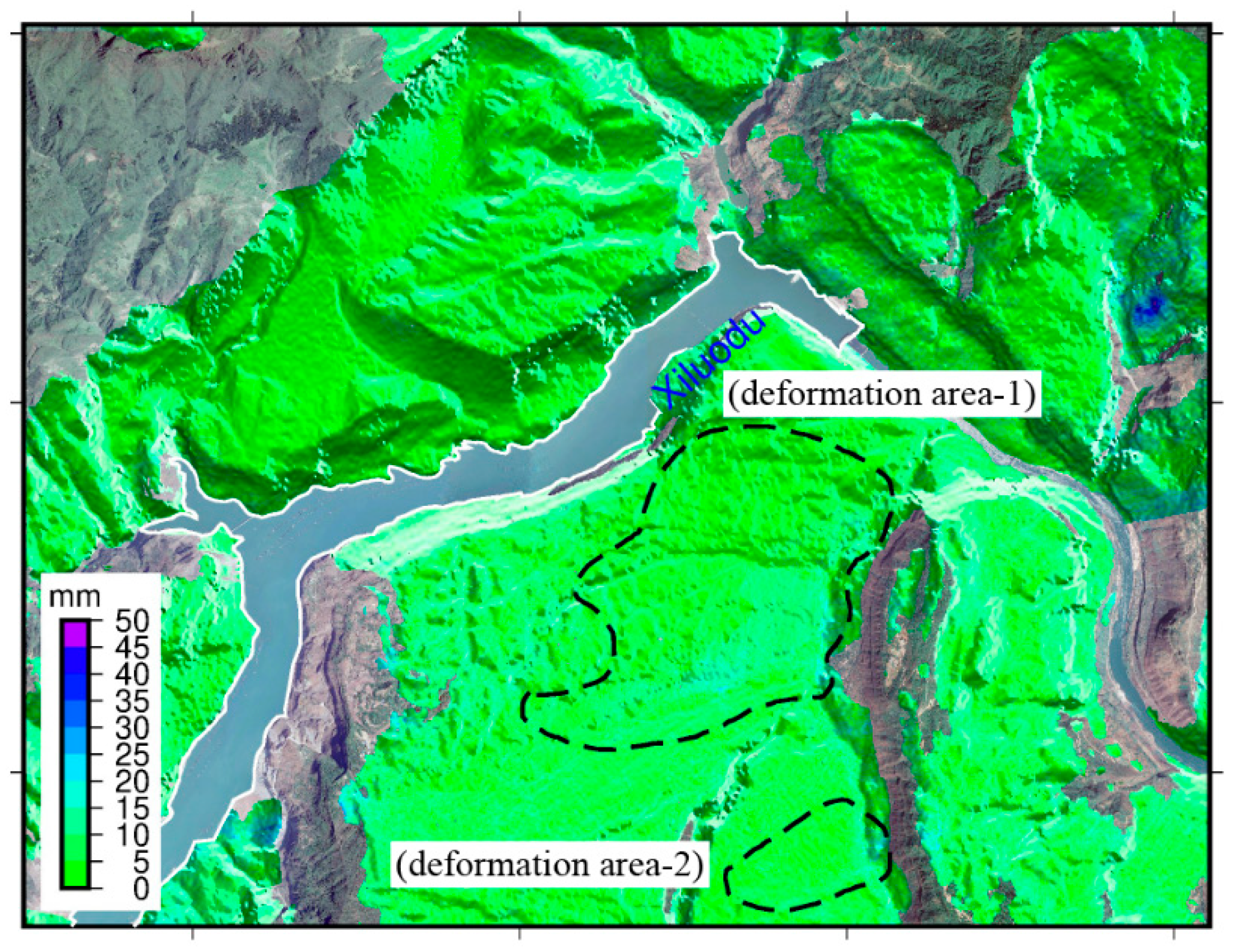
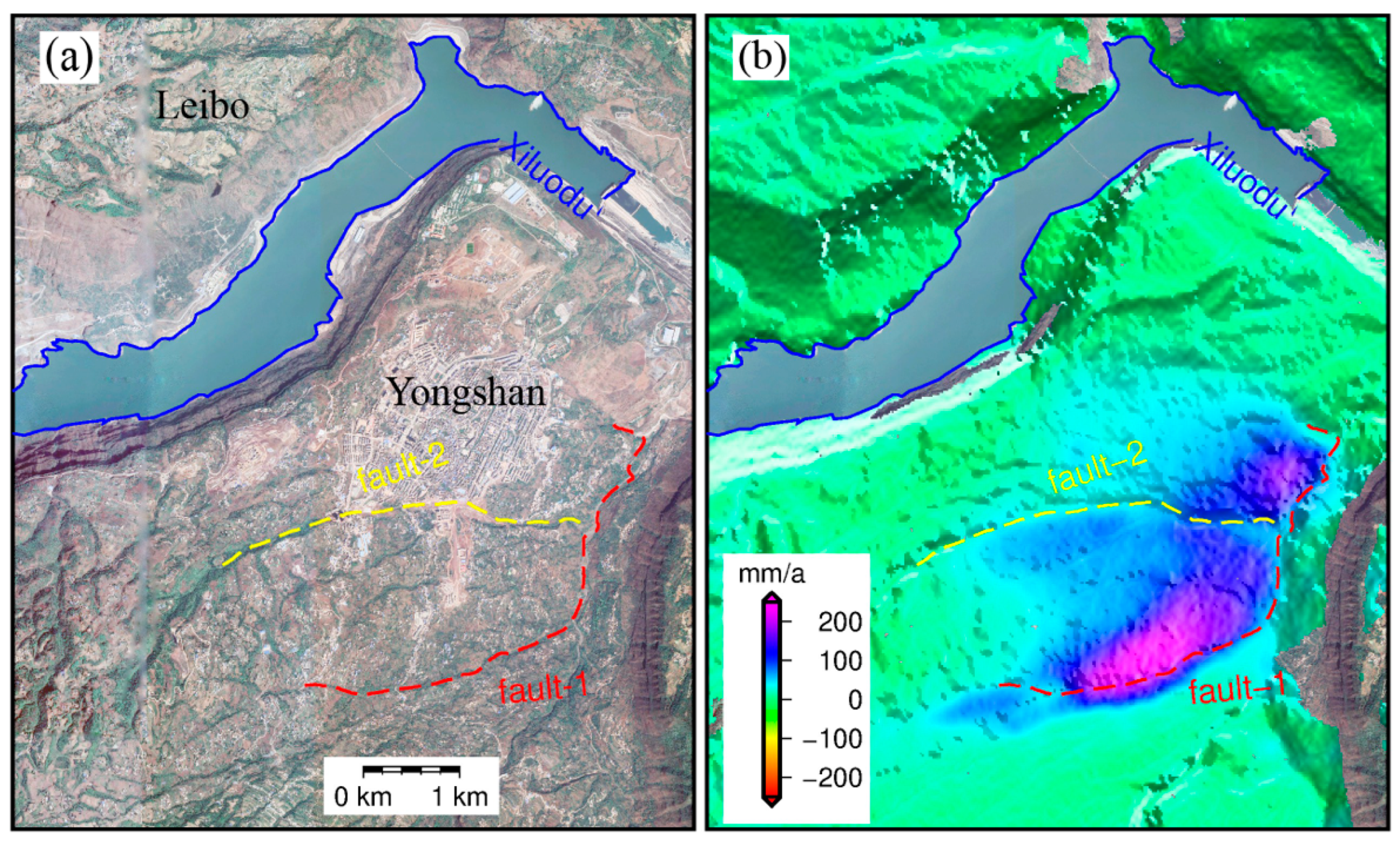
5.3. Potential Geological Hazards

According to the National Geological Hazard Bulletin, there were 2966 geological disasters in 2018, resulting in 105 deaths and seven missing people. The direct economic losses amounted to RMB 1.47 billion. Among them, the southwestern region suffered the most serious disasters, accounting for 35.2% of national geological disasters. Therefore, monitoring geological disasters is vital. As a wide-ranging monitoring method, InSAR can undoubtedly provide necessary observation of geological disasters. However, due to the limitation of satellite side-view imaging, the SAR satellite of a single platform may have overlapping, shadow, and top–bottom inversion in complex mountainous areas, which may easily cause blind spots of identification, resulting in misjudgment [37]. Therefore, through a variety of data (ascending and descending data), the true strength of InSAR technology can be realized in complex mountainous areas. In this paper, we used the data of multiple orbits to decompose the study area horizontally and vertically, thus restoring the deformation of the entire study area. According to the analysis in Section 5.1, combined with the optical image (as shown in Figure 17a), we found that the deformation of the trailing edge (fault-1) of the significant region of deformation was large, and then through the analysis in Section 5.2, we speculate that the region will continue to move along the coast, which may lead to cracks at the trailing edge, and the formation of geological disasters such as ground fissures and collapses, which require following up. At the same time, the left side of the area has a distinct block in the deformed area on the right. As the deformation in the horizontal direction continues to accumulate, the unequal horizontal forces in the two areas may cause relative shear, causing the middle area to form a fault (Fault-2), which may lead to geological disasters such as landslides and ground fissures. As can be seen from the foregoing, the geological conditions in the area are relatively fragile. Therefore, in order to avoid large casualties, the area should be continuously monitored.

6. Conclusions

As China’s demand for power resources continues to increase, hydropower has become increasingly important as a clean and recyclable energy source. However, the artificial construction of a reservoir undoubtedly changes the hydrogeological conditions of the hydropower station’s attached structures, resulting in deformation of the surface near the hydropower station, which can lead to landslides, mudslides, earthquakes, etc. In this paper, using time-series InSAR technology, through a variety of data (ALOS2 ascending, Sentinel-1 ascending and descending), large-scale surface deformation monitoring was carried out near the Xiluodu reservoir area after water storage and power generation. The conclusions are as follows:

(1)

For a variety of data, the space is not synchronized, and the deformation sequence decomposition cannot be directly performed. A new solution was proposed, and the horizontal and vertical deformation values of the entire time series were obtained. The results show that the maximum average velocity is perpendicular to the bank edge, the maximum average velocity is 250 mm/a, and the maximum vertical velocity is 60 mm/a, which indicates that the surface deformation near the Xiluodu reservoir area is mainly horizontal and the vertical direction is supplemented. At the same time, we used the residuals to analyze the accuracy of the deformation solution. The results show that the deformation accuracy can reach 10 mm within the 95% confidence interval, indicating that the accuracy of this experiment is reliable.

(2)

By analyzing the relationship between horizontal displacement and vertical displacement and water level, it was found that after the Xiluodu water storage, the vertical bank direction displacement continued to increase. This indicates that the deformation caused by the water storage was not due to the elastic displacement caused by the load but caused instead by the irreversible shaping displacement. According to its development trend, we speculate that the vertical shore direction displacement will continue to increase and finally stabilize. According to its development trend, we speculate that the displacement in the vertical shore direction will continue to increase and finally stabilize; the displacement in the vertical direction increases rapidly at the initial stage of water storage. After two water-storage cycles, the vertical deformation begins to stabilize, and the vertical deformation will change with the change in storage period.

(3)

Through the analysis of the results and potential faults, we speculate that there may be two faults at this location. As the horizontal deformation continues to accumulate, it may cause cracking, which will aggravate the geological vulnerability of the site.

This experiment failed to obtain GPS data, so it is impossible to verify the decomposition results of InSAR data with external data. At the same time, the acquisition date of this experimental data was after the Xiluodu Hydropower Station started operating. In subsequent analysis, we can try to obtain the InSAR data before the Xiluodu Reservoir was stored and thus gain a clearer understanding of the landmark deformation near the Xiluodu Reservoir.

References

1. Bartle, A. Hydropower potential and development activities. Energy Policy 2002, 30, 1231–1239. [Google Scholar] [CrossRef]
2. Hennig, T.; Wang, W.; Feng, Y.; Xiaokun, O.U.; Daming, H.E. Review of Yunnan’s hydropower development. Comparing small and large hydropower projects regarding their environmental implications and socio-economic consequences. Renew. Sustain. Energy Rev. 2013, 27, 585–595. [Google Scholar] [CrossRef]
3. Wang, L.; Chao, C.; Rong, Z.; Du, J. Surface gravity and deformation effects of water storage changes in China’s Three Gorges Reservoir constrained by modeled results and in situ measurements. J. Appl. Geophys. 2014, 108, 25–34. [Google Scholar] [CrossRef]
4. Xiao Shirong, L.D.; Hu, Z. Engineering geologic study of three actual dip bedding rockslides associated with reservoirs in world. J. Eng. Geol. 2010, 18, 52–59. [Google Scholar]
5. Bosa, S.; Petti, M. Shallow water numerical model of the wave generated by the Vajont landslide. Environ. Model. Softw. 2011, 26, 406–418. [Google Scholar] [CrossRef]
6. Zhang, L.; Liao, M.; Balz, T.; Shi, X.; Jiang, Y. Monitoring Landslide Activities in the Three Gorges Area with Multi-frequency Satellite SAR Data Sets. In Modern Technologies for Landslide Monitoring and Prediction; Springer: Berlin/Heidelberg, Germany, 2015; pp. 181–208. [Google Scholar]
7. Pingue, F.; Obrizzo, F.; Serio, C. Vertical ground movements in the Colli Albani area (central Italy) from recent precise levelling. Appl. Geomat. 2013, 5, 203–214. [Google Scholar] [CrossRef]
8. Fastellini, G.; Radicioni, F.; Stoppini, A. The Assisi landslide monitoring: A multi-year activity based on geomatic techniques. Appl. Geomat. 2011, 3, 91–100. [Google Scholar] [CrossRef]
9. Barazzetti, L.; Gianinetto, M.; Scaioni, M. A New Approach to Satellite Time-series Co-registration for Landslide Monitoring. In Modern Technologies for Landslide Monitoring and Prediction; Springer: Berlin/Heidelberg, Germany, 2015. [Google Scholar]
10. Liu, P.; Li, Z.; Hoey, T.; Kincal, C.; Zhang, J.; Zeng, Q.; Muller, J.P. Using advanced InSAR time series techniques to monitor landslide;movements in Badong of the Three Gorges region, China. Int. J. Appl. Earth Obs. Geoinf. 2013, 21, 253–264. [Google Scholar] [CrossRef]
11. Massonnet, D.; Feigl, K.L.; Massonnet, D.; Feigl, K.L. Radar interferometry and its application to changes in the Earth’s surface. Rev. Geophys. 1998, 36, 441–500. [Google Scholar] [CrossRef] [Green Version]
12. Fruneau, B.; Achache, J.; Delacourt, C. Observation and Modelling of the Saint-Etienne-de-Tinée Landslide Using SAR Interferometry. Tectonophysics 1996, 265, 181–190. [Google Scholar] [CrossRef]
13. Simons, M.; Fialko, Y.; Rivera, L. Coseismic Deformation from the 1999 Mw 7.1 Hector Mine, California, Earthquake as Inferred from InSAR and GPS Observations. Bull. Seismol. Soc. Amer. 2002, 92, 1390–1402. [Google Scholar] [CrossRef]
14. Hooper, A.; Zebker, H.; Segall, P.; Kampes, B. A new method for measuring deformation on volcanoes and other natural terrains using InSAR persistent scatterers. Geophys. Res. Lett. 2004, 31, L23611. [Google Scholar] [CrossRef]
15. Bing, X.; Feng, G.; Li, Z.; Wang, Q.; Wang, C.; Xie, R. Coastal Subsidence Monitoring Associated with Land Reclamation Using the Point Target Based SBAS-InSAR Method: A Case Study of Shenzhen, China. Remote Sens. 2016, 8, 652. [Google Scholar]
16. Zebker, H.A.; Villasenor, J. Decorrelation in interferometric radar echoes. IEEE Trans. Geosci. Remote Sens. 1992, 30, 950–959. [Google Scholar] [CrossRef] [Green Version]
17. Li, Z.W.; Xu, W.B.; Feng, G.C.; Hu, J.; Wang, C.C.; Ding, X.L.; Zhu, J.J. Correcting atmospheric effects on InSAR with MERIS water vapour data and elevation-dependent interpolation model. Geophys. J. Int. 2012, 189, 898–910. [Google Scholar] [CrossRef] [Green Version]
18. Ferretti, A.; Prati, C.; Rocca, F. Nonlinear subsidence rate estimation using permanent scatterers in differential SAR interferometry. IEEE Trans. Geosci. Remote Sens. 2000, 38, 2202–2212. [Google Scholar] [CrossRef] [Green Version]
19. Mora, O.; Lanari, R.; Mallorquί, J.J.; Berardino, P. A new algorithm for monitoring localized deformation phenomena based on small baseline differential SAR interferograms. In Proceedings of the IEEE International Geoscience & Remote Sensing Symposium, Toronto, ON, Canada, 24–28 June 2002. [Google Scholar]
20. Zhao, C.Y.; Kang, Y.; Zhang, Q.; Zhu, W.; Li, B. Landslide detection and monitoring with InSAR technique over upper reaches of Jinsha River, China. In Proceedings of the IGARSS 2016, Beijing, China, 10–15 July 2016. [Google Scholar]
21. Yin, Y.; Sun, P.; Zhu, J.; Yang, S. Research on catastrophic rock avalanche at Guanling, Guizhou, China. Landslides 2011, 8, 517–525. [Google Scholar] [CrossRef]
22. Liang, G.H.Y.; Fan, Q.; Li, Q. Analysis on valley deformation of Xiluodu high arch dam during impoundment and its influence factors. J. Hydroelectr. Eng. 2016, 35, 101–110. [Google Scholar]
23. Zhou, Z.L.M.; Zhuang, C.; Guo, Q. Impact factors and forming conditions of valley deformation of Xiluodu Hydropower Station. J. Hohai Univ. (Nat. Sci.) 2018, 46, 497–505. [Google Scholar]
24. Li, L.Y.X.; Zhou, Z.; Feng, X.; Liu, X. The deformation characteristics of a large landslide before and after impoundment in the xiluodu area based on insar technology. In Proceedings of the 2017 National Engineering Geology Academic Annual Meeting, Guilin, China, 28–29 October 2017; p. 5. [Google Scholar]
25. Li, L.; Yao, X.; Yao, J.; Zhou, Z.; Feng, X.; Liu, X. Analysis of deformation characteristics for a reservoir landslide before and after impoundment by multiple D-InSAR observations at Jinshajiang River, China. Nat. Hazards 2019, 98, 719–733. [Google Scholar] [CrossRef]
26. Zhu, Y.; Yao, X.; Yao, L.; Zhou, Z.; Ren, K.; Li, L.; Yao, C.; Gu, Z. Identifying the Mechanism of Toppling Deformation by InSAR: A Case Study in Xiluodu Reservoir, Jinsha River. Landslides 2022, 19, 2311–2327. [Google Scholar] [CrossRef]
27. Zhongli, R. Main Environmental Problems at Xiluodu Waterpower Project. Sichuan Water Power 1994, 40–47 + 94. [Google Scholar]
28. Hongyan, D.W.C. Analysis on Engineering Geological Characteristics and Genesis Mechanism of Ku’an Lao Landslide in Xiluodu Reservoir Area. Soil Water Conserv. China 2011, 59–62. [Google Scholar]
29. Wu, D.C.; Li, Y.S.; Liu, W.L.; Deng, J.H.; Wang, D.Y.; Xiao, Y.F. Activity of the Majiahe Dam fault and stability of engineering works in the Xiluodu Hydropower Station in the lower reaches of the Jinsha River, southwestern China. Geol. Bull. China 2006, 25, 506–511. [Google Scholar]
30. Hu, J.; Li, Z.W.; Ding, X.L.; Zhu, J.J.; Zhang, L.; Sun, Q. Resolving three-dimensional surface displacements from InSAR measurements: A review. Earth-Sci. Rev. 2014, 133, 1–17. [Google Scholar] [CrossRef]
31. Hu, J.; Li, Z.W.; Zhu, J.J.; Zhang, L.; Sun, Q. 3D coseismic Displacement of 2010 Darfield, New Zealand earthquake estimated from multi-aperture InSAR and D-InSAR measurements. J. Geod. 2012, 86, 1029–1041. [Google Scholar] [CrossRef]
32. Samsonov, S.V.; D’Oreye, N. Multidimensional Small Baseline Subset (MSBAS) for Two-Dimensional Deformation Analysis: Case Study Mexico City. Can. J. Remote Sens. 2017, 43, 318–329. [Google Scholar] [CrossRef]
33. Pepe, A.; Solaro, G.; Calo, F.; Dema, C. A Minimum Acceleration Approach for the Retrieval of Multiplatform InSAR Deformation Time Series. IEEE J. Sel. Top. Appl. Earth Obs. Remote Sens. 2016, 9, 3883–3898. [Google Scholar] [CrossRef]
34. Xuguo Shi, L.Z.; Zhou, C.; Li, M.; Liao, M. Retrieval of time series three-dimensional landslide surface displacements from multi-angular SAR observations. Landslides 2018, 15, 1015–1027. [Google Scholar]
35. Aster, R.C.; Borchers, B.; Thurber, C.H. Parameter Estimation and Inverse Problems; Elsevier: Amsterdam, The Netherlands, 2018. [Google Scholar]
36. Li, M.; Zhang, L.; Shi, X.; Liao, M.; Yang, M. Monitoring active motion of the Guobu landslide near the Laxiwa Hydropower Station in China by time-series point-like targets offset tracking. Remote Sens. Environ. 2019, 221, 80–93. [Google Scholar] [CrossRef]
37. Zhao, C.; Liu, X.; Zhang, Q.; Peng, J.; Xu, Q. Research on Loess Landslide Identification, Monitoring and Failure Mode with InSAR Technique in Herfangtai, Gansu. Geomat. Inf. Sci. Wuhan Univ. 2019, 44, 996–1007. [Google Scholar]
Figure 1. Topography profile of Western—Eastern China.
Remotesensing 15 00168 g001
Figure 2. Basic geological structural map of Xiluodu area. F1 is the Majingzi fault, F2 is the Jiziba fault, and F3 is the Majiahe fault.
Remotesensing 15 00168 g002
Figure 3. (a) Water level of Xiluodu reservoir; (b) distribution of aquifers (along the red line in Figure 2) of Xiluodu after water impoundment. A is the river reservoir, B is the area of Yongshan County. S is the Rammell aquifuge layer; P1 m is the limestone permeable bed layer; P2βn is the Rammell aquifuge layer; P2β is the basalt permeable bed layer; P2x is the sandy shale layer; Q is the Quaternary loose accumulation layer; the green arrow indicates the direction of water flow; the red arrow indicates the direction of deformation along the Jinsha River valley. L1 is the water level before constructing Xiluodu Hydropower Station, and L2 is the water level after its construction.
Remotesensing 15 00168 g003
Figure 4. Schematic diagram of LOS decomposition. The red arrow represents the local east, north, up (ENU) coordinates; the blue arrow represents the flight direction of the satellite; the green arrow indicates the LOS direction; φ and θ are the azimuth and incident angle of the satellite, respectively; δ is the azimuth angle of a predefined direction; n and p directions are defined local coordinate systems.
Remotesensing 15 00168 g004
Figure 5. Time series of Sentinel-1 ascending and descending data, and ALOS2 ascending data.
Remotesensing 15 00168 g005
Figure 6. Flowchart of the proposed method.
Remotesensing 15 00168 g006
Figure 7. (a) Study area; (b) SAR data coverage area. The white dashed box represents the Sentinel-1 ascending data, and the black dashed box represents the Sentinel-1 descending data. The blue dashed box represents the ALOS2 ascending data.
Remotesensing 15 00168 g007
Figure 8. Two-connection network mode. The black triangles represent the SAR images in chronological order from left to right, and the red lines represent different interference pairs.
Remotesensing 15 00168 g008
Figure 9. (a) Mean velocity map of ALOS2 ascending; (b) mean velocity map of Sentinel-1 ascending; (c) mean velocity map of Sentinel-1 descending.
Remotesensing 15 00168 g009
Figure 10. (a) Mean rate perpendicular to the shore direction; (b) vertical mean rate.
Remotesensing 15 00168 g010
Figure 11. (a) Horizontal time-series deformation; (b) vertical time-series deformation.
Remotesensing 15 00168 g011
Figure 12. (a) is the horizontal displacement rate of profile line A–B; (b) is the vertical displacement rate of profile line A–B; (c) is the horizontal displacement rate of profile line C–D; (d) is the vertical displacement rate of profile line C–D; (e) is the horizontal displacement rate of profile line E–F; (f) is the vertical displacement rate of profile line E–F. The green line represents the suspected fault.
Remotesensing 15 00168 g012
Figure 13. Root mean square error chart. (a) Total mean square error; (b) deformation significant regional mean square error; (c) deformation non-significant area mean square error.
Remotesensing 15 00168 g013
Figure 14. Overall root mean square error map.
Remotesensing 15 00168 g014
Figure 15. Relationship between horizontal displacement and impoundment. (a) is the relationship between the deformation sequence and water level in the horizontal direction of point P1 in Figure 10; (b) is the deformation sequence in (a) that removes the linear trend; (c) is the relationship between the deformation sequence and water level in the horizontal direction of point P2 in Figure 10; (d) is the deformation sequence in (c) that removes the linear trend.
Remotesensing 15 00168 g015
Figure 16. Relationship between vertical displacement and water storage. (a) is the relationship between the deformation sequence and water level in the vertical direction of point P1 in Figure 10; (b) is the deformation sequence in (a) that removes the linear trend; (c) is the relationship between the deformation sequence and water level in the vertical direction of point P2 in Figure 10; (d) is the deformation sequence in (c) that removes the linear trend.
Remotesensing 15 00168 g016
Figure 17. (a) Optical image; (b) potential fault.
Remotesensing 15 00168 g017