Multi-Scale Response Analysis and Displacement Prediction of Landslides Using Deep Learning with JTFA: A Case Study in the Three Gorges Reservoir, China

Abstract

Reservoir water and rainfall, leading to fluctuations groundwater levels, are the main triggering factors that induce landslides in the Three Gorges Reservoir area. This study investigates the response mechanism of landslide deformation under reservoir water and rainfall variations through long-time on-site observations. To address the non-stationary characteristics of the time-series records, joint time-frequency analysis (JTFA) is first introduced into our landslide prediction model. This model employs optimal variational mode decomposition (VMD) to obtain specific signal components with clear physical meaning, such as trend component and periodic components. Then, multi-scale response analysis between the displacement and external factors three wavelet methods was conducted. The analysis results show a 1 year primary cycle of the time series associated with the landslide evolution. The reservoir water level and rainfall show anti-phase fluctuations. The periodic displacement correlates significantly with rainfall, lagging by about two months. The reservoir water is anti-phase with the landslide displacement, preceding it by approximately three months (−51 ± 8° phase difference). For landslide displacement prediction, the gated recurrent units (GRU) neural network model is integrated into the deep learning forecasting architecture. The model takes into account the correlation and hysteresis effect of input variables. Through six experiments, we investigate the effect of data volume on model predictions to determine the optimal model. The results demonstrate that our proposed model ensures high performance in landslide prediction. Moreover, a comparison with six other intelligent algorithms shows the advantages of our model in terms of time-effectiveness and long-sequence forecasting.

1. Introduction

Since the Three Gorges Reservoir (TGR) was put into operation in June 2003, the stability of slopes along the TGR bank has changed dramatically in response to the periodic fluctuation of the rainfall intensity and the reservoir storage [1,2,3], resulting in thousands of reactivated landslides. The geomechanical and hydrologic characteristics of these landslides are continually affected by the consistent water levels and rainfall changes, leading to catastrophic events [4]. For example, the July 2003 Qianjiangping landslide developed during the initial reservoir impoundment, causing 24 fatalities and significant economic losses [5]. Since then, research on long-term monitoring and early warning of these landslides has steadily expanded, leading to a deeper understanding of the inherent patterns and the response mechanism of reservoir landslides.

Studies have revealed that the evolution of the reservoir landslide involves a complex, non-stationary and nonlinear dynamic process [6,7]. Consequently, the long-term observations collected on the landslide’s behavior exhibit non-stationary time-varying characteristics with specific trends and/or seasonality. Although the deformation evolution and response analysis of reservoir landslides in TGR have been extensively studied and discussed in the time domain [8,9,10], their characteristics in the frequency domain are relatively unexplored, concealing valuable spectral information. Furthermore, non-stationary time series show time-frequency characteristics [6,11,12], making time-frequency representation of the signal essential for identifying the dominant fluctuation modes/spectra of different signals and understanding how those modes vary over time.

The empirical mode decomposition (EMD), developed by Huang et al. [13], is well-known for its time-frequency analysis, which is suitable for processing non-stationary time series. This method decomposes the data into different band-limited intrinsic mode functions (IMFs), but is sensitive to noise and sampling [14]. The variational modal decomposition (VMD), a more recent signal decomposition technique, enables fully intrinsic and adaptive decomposition [14]. In addition, Isham et al. also pointed out the importance of determining the number of VMD modes to obtain specific signal components with explicitly physical meaning [15]. To achieve efficient decomposition, the Shannon entropy, reflecting the uniformity of probability distribution, can be used as a fitness function to derive optimal parameters through an optimization method, such as the harmony search (HS) algorithm [16] and the wolf optimization algorithm (GWO) [17] employed in this study. GWO is easily implemented and exhibits advantages in strong convergence with few parameters.

Moreover, it is crucial to explore the response mechanisms of landslide deformation [18] to unveil the changing patterns of specific signal components at different scales. In 1998, Torrence et al. proposed wavelet analysis (WA) to study non-stationary time series in signal processing [19]. Presently, wavelet decomposition and denoising are the most popular WA methods in time series analysis widely used in Geophysics [19], Geography [20] and Meteorology [21]. However, WA methods, such as continuous wavelet transform (CWT), cross-wavelet transform (XWT) and wavelet coherency (WTC), are more suitable for analyzing non-stationary time series at different scales [7,22,23,24]. Unfortunately, they are rarely used to analyze long-term non-stationary observations associated with landslide behavior. As a result, this study will extend WA methods and optimized VMD into a deep learning framework to conduct a joint time-frequency analysis (JTFA) before establishing a landslide forecasting model.

So far, various approaches have been developed for landslide hazards research, ranging from physics-based to statistics-based models [9,25,26]. Over the past decades, the integration of machine learning (ML) methods into landslide research has led to significant advancements [2,8,9]. In recent years, deep-learning approaches, like recurrent neural networks (RNN) and their variants, designed to address the gradient explosion problem, have shown impressive success in predicting landslide displacements based on GNSS time series data [4,10,27,28]. Among these variants, the gated recurrent unit (GRU) proposed by Chung et al. [29] stands out, surpassing other RNN variants, such as the LSTM, in terms of training time, parameter update and generalization ability. Its outstanding performance extends to diverse fields, including economics [30], flood control [31] and disaster reduction [10], among others.

This paper presents a deep learning neural network model for predicting landslide displacement, incorporating a joint time-frequency analysis (JTFA) module. The JTFA employs optimal variational mode decomposition (VMD) to obtain specific signal components with clear physical meaning (e.g., trend component and periodic component). Subsequently, multi-scale response analysis between the displacement and external factors is carried out by wavelet transform (CWT), cross-wavelet transform (XWT) and wavelet coherency (WTC). The enhanced GRU model based on deep learning architecture is employed to forecast landslide displacement (Figure 1e–g). Additionally, the model considers the correlation and hysteresis effect of input variables, such as impact factors, during the modeling process.

2. Methodology

As can be seen in Figure 1, the forecasting model consists of seven parts: Figure 1 (a) signal decomposition of landslide displacement, Figure 1 (b) signal decomposition of the impacting factors, Figure 1 (c) multi-scale response analysis of landslide deformation by JTFA, Figure 1 (d) data packet preparation for the deep-learning neural network model, Figure 1 (e) trend displacement prediction by DES, Figure 1 (f) periodic and random displacement prediction by GRU, and Figure 1 (g) cumulative displacements prediction by the optimal model.

First, the on-site measured landslide displacements and the pre-selected impact factor sequences are decomposed into specific IMF components by an optimal VMD (Figure 1a,b). The number and parameters of the VMD modes with explicit physical meanings are determined by employing the Shannon entropy as a fitness function and the GWO optimization method. Then, a multi-scale response analysis between the displacement and external factors is carried out by three wavelet analysis methods to investigate landslide deformation response mechanisms and to reveal the changing patterns of specific signal components at different scales (Figure 1c). Finally, the enhanced GRU and DES model based on deep learning architecture is used to predict the landslide displacement (Figure 1e–g).

2.1. Joint Time-Frequency Analysis (JTFA)

The collected long-term observations associated with the landslide’s behavior are non-stationary time series with specific trends or/and seasonality. The landslide displacement is a time-series function controlled by geological conditions, reflecting long-term deformation trends. While subject to external influences, the landslide displacement behaves as a periodic variation with near-white noise associated with random factors. Therefore, the landslide displacement time series can be expressed as follows:

$$Y_t=T_t+P_t+R_t$$

(1)

where Y_t is the landslide displacement at time t; while T_t, P_t and R_t are the trend, periodic and random terms, respectively.

While studies on the deformation characteristics of landslides have been extensively explored in the time domain, the significance of time-frequency analysis of the signal should not be overlooked. Time-frequency analysis reveals the time-frequency features, and it provides access to the implicit spectral information of displacement Y_t with different spectra, enabling a time-frequency perspective of information mining. Having a time-frequency representation is indispensable to investigate the dominant fluctuation spectra of deformation signals and understand how those spectra vary over time. This involves one-dimensional time series converting into a diffuse two-dimensional time-frequency image, allowing for a comprehensive examination of the signal’s temporal and frequency properties.

2.1.1. Grey Wolf Optimized Variational Mode Decomposition (GWO-VMD)

The VMD enables fully intrinsic and adaptive signal decomposition [14], by which the input displacement signal could be divided into several intrinsic mode functions (IMFs) with specific characteristics determined in advance. To ensure that (1) the central frequency bandwidth of each IMF is limited, (2) the sum of the estimated bandwidths is minimized, and (3) the sum of each IMF equals the original signal f so that the constrained variational equation can be expressed as follows:

$$\begin{array}{l}\underset{\left\{u_k\right\},\left\{w_k\right\}}{\min }\left\{{\displaystyle \sum _k{\Vert {\partial }_t\left[\left(\delta \left(t\right)+j/\pi t\right)\ast u_k\left(t\right)\right]e^{-j{\omega }_{k}t}\Vert }_2^2}\right\}\\ s.t. \hspace{1em} {\displaystyle \sum _k^K{u}_k=f}\end{array}$$

(2)

where u_k is the kth decomposed IMF with a center frequency w_k; and δ(t) and * indicate the Dirac function and the convolution operator, respectively.

Then, the Lagrange multipliers λ and decomposition parameter ε are introduced to transform the constrained problem into an unconstrained variational one, yielding the augmented Lagrange expression:

$$\begin{array}{l}L\left(\left\{u_k\right\},\left\{{\omega }_k\right\},\lambda \right)=\\ \epsilon {\displaystyle \sum _k{\Vert {\partial }_t\left[\left(\delta \left(t\right)+j/\pi t\right)\ast u_k\left(t\right)\right]e^{-j{\omega }_{k}t}\Vert }_2^2}+\\ {\Vert f\left(t\right)-{\displaystyle \sum _k{u}_k\left(t\right)}\Vert }_2^2+\langle \lambda \left(t\right),f\left(t\right)-{\displaystyle \sum _k{u}_k\left(t\right)}\rangle \end{array}$$

(3)

Here, the alternating direction multiplier method (ADMM) is used to search the saddle points of the unconstrained model to obtain the optimal IMFs and the center frequency of the constrained model. This process is defined as a function f_VMD in the Algorithm 1.

The VMD is used to decompose complex digital signals, and the empirical decomposition parameter ε is usually K > 3. This value will not be physically meaningful when applied to the landslide displacement decomposition. Thus, obtaining suitable VMD modes is crucial to getting specific signal components with explicitly physical meaning. At this point, the Shannon entropy (Equation (4)) is introduced to obtain the optimal IMFs with sparse features: the larger the value is, the better the uniformity of the probability distribution is [32].

$$H\left(u_k\right)=-{\displaystyle \sum _{i=1}^n{u}_k^i\log u_k^i}$$

(4)

As for the landslide’s periodic displacement, the probability distribution is relatively uniform and sparse. Thus, the value of ε is optimized using the grey wolf optimizer (GWO) with H(u_k) as the fitness function [26] to obtain the periodic displacement with a uniform probability distribution and strong sparsity along with the trend and random terms.

The landslide displacement Y_t is used as input. The population size P of the grey wolf, the upper bound X_up and lower bound X_low of the individual grey wolves are initialized. Then, the algorithm iterates and updates N times to obtain the optimal value of ε (see the Algorithm 1). In the Algorithm 1, both A and C are coefficient vectors with $A=2a\cdot r_1-a$ and $C=2\cdot r_2$. r₁ and r₂ are random values between 0 and 1. The convergence factor, $a=2-2\mathrm{n}/N$, decreases linearly from 2 to 0 during the iteration.

Algorithm 1 The GWO-VMD

Initialize ${\epsilon }_{\alpha },{\epsilon }_{\beta },{\epsilon }_{\delta },n \leftarrow 0$ ${\epsilon }_p^1 \leftarrow X_{low}+\left(X_{up}-X_{low}\right)\times rand\left(0,1\right)$      (5) repeat $n \leftarrow n+1$ $\left\{u_k^p\right\} \leftarrow f_{VMD}\left(Y_t,{\epsilon }_p^n\right)$                 (6) Update ${\epsilon }_{\alpha },{\epsilon }_{\beta },{\epsilon }_{\delta }$: ${\epsilon }_{\alpha },{\epsilon }_{\beta },{\epsilon }_{\delta } \leftarrow \underset{1,2,3}{\max }H\left(\left\{u_{k=2}^p\right\}\right)$              (7) for $p=1:P$   do                     Update ${\epsilon }_p$: $X_1 \leftarrow {\epsilon }_{\alpha }-A_1\left|C_1{\epsilon }_{\alpha }-{\epsilon }_p^n\right|$                 (8) $X_2 \leftarrow {\epsilon }_{\beta }-A_2\left|C_2{\epsilon }_{\beta }-{\epsilon }_p^n\right|$                 (9) $X_3 \leftarrow {\epsilon }_{\delta }-A_3\left|C_3{\epsilon }_{\delta }-{\epsilon }_p^n\right|$                 (10) ${\epsilon }_p^{n+1} \leftarrow mean\left(X_1,X_2,X_3\right)$                   (11) end for until $n=N$.

2.1.2. Wavelet Analysis (WA)

Torrence and Compo [22] proposed WA to study non-stationary time series in signal processing. The most popular WA methods in time series analysis include wavelet decomposition and denoising. Additionally, there are other WA methods, such as the continuous wavelet transform (CWT), the cross-wavelet transform (XWT) and the wavelet coherency (WTC), which excel at non-stationary time series analysis at various scales. However, despite their effectiveness, these WA methods are still rarely used in non-stationary time series analysis associated with the behavior of landslides.

For a discrete time-series x_n (n = 1, …, N) with equal time spacing δt, the CWT is used for mapping the changing properties of non-stationary signals. CWT is defined as the convolution of x_n with a scaled and translated version of the wavelet basis function:

$$W_n(s)={\displaystyle \sum _{n^{\prime }=1}^{N-1}{x}_{n^{\prime }}\psi \ast \left[\frac{\left(n^{\prime }-n\right)\delta t}{s}\right]}$$

(12)

where * indicates the complex conjugate, s represents the wavelet scale, and n is the localized time index. The non-orthogonal Morlet wavelets are chosen as the basis function: ${\psi }_0\left(\eta \right)={\pi }^{-1/4}{e}^{i{w}_0\eta }{e}^{-{\eta }^2/2}$, where $\eta$ and $w_0$ are non-dimensional parameters of time and frequency, respectively. When w₀ = 6, the wavelet scale s equals the Fourier period. The wavelet basis functions ${\psi }_0$ are then normalized to have unit energy, and the CWT is conducted in the Fourier space to improve efficiency.

In Equation (12), W_n(s) is a complex value, and thus, |W_n(s)|² denotes the wavelet power spectrum that clearly discriminates the periodic fluctuation and intensity in the time series. As the input data is assumed to be cyclic, edge effects appear in the power spectrum when dealing with finite-length time series. Hence, the cone of influence (COI) is defined, representing the corresponding edge effects within the region of the power spectrum. In addition, a Fourier power spectrum is constructed by Monte Carlo to represent the red noise background spectrum and later performs a χ² test with a specific confidence level, e.g., 95%, to calculate each scale and construct the confidence contour with a 95% confidence level.

The XWT of two time-series x_n and y_n is defined as W^XY = W^XW^Y*, which measures the similarity between two waveforms. The arg(W^XY) is the relative local phase between x_n and y_n in the time-frequency space. The mean and confidence interval must be estimated to analyze the phase difference. The phase relation is quantified using the periodic mean of phases over a region with a significance level of 5% outside the COI. The periodic mean of a set of phase angles is defined as follows:

$$a_m=\arg \left(X,Y\right) \mathrm{with} X={\displaystyle \sum _{i=1}^n\cos \left({\alpha }_i\right)} \mathrm{and} Y={\displaystyle \sum _{i=1}^n\sin \left({\alpha }_i\right)}$$

(13)

Because the phase angles are not independent, it is difficult to calculate the confidence interval of the mean angle. Thus, the solution is obtained by calculating the scatter around the mean using the circular standard deviation $er=\sqrt{-2\ln \left(\sqrt{X^2+Y^2}/n\right)}$.

The power spectrum of XWT only shows the high common power part, while the WTC measures the coherence of the XWT in the time-frequency space. The WTC of two-time series is defined as follows:

$$R_n^2\left(s\right)=\frac{{\left|S\left(s^{-1}{W}_n^{XY}\left(s\right)\right)\right|}^2}{S\left(s^{-1}{\left|W_n^X\left(s\right)\right|}^2\right)\cdot S\left(s^{-1}{\left|W_n^Y\left(s\right)\right|}^2\right)}$$

(14)

where S is the smooth operator, and S(W) = S_scale(S_time(W_n(S))). S_scale and S_time indicate smoothing along the wavelet scale axis and over time, separately.

2.2. Deep Learning Forecasting Model

2.2.1. Gated Recurrent Unit (GRU)

The gated recurrent unit (GRU) is a variant of recurrent neural networks (RNN), which outperforms other RNN variants, e.g., the LSTM [29], in terms of training time, and has fewer parameters. The GRU enables each recurrent unit to capture dependencies adaptively at different time scales. As a refinement of the general RNN structure, GRU is more straightforward, owing to the absence of a separate storage unit (see Figure 2) regulating the internal information flow via a gated unit. Moreover, it is more efficient in training time, parameter update and generalization ability than other RNNs [29].

The update gate z_t is responsible for determining how much of the past information is to be neglected, while the reset gate r_t is responsible for deciding how much past knowledge needs to be passed along into the future. Assume that the current input at t is x_t, then one forward calculation of GRU is as follows:

$$z_t=\sigma \left(W_z\cdot \left[h_{t-1},x_t\right]+b_z\right)$$

(15)

$$r_t=\sigma \left(W_r\cdot \left[h_{t-1},x_t\right]+b_r\right)$$

(16)

$${\tilde{h}}_t=\tanh \left(W_{\tilde{h}}\cdot \left[r_t\ast h_{t-1},x_t\right]+b_{\tilde{h}}\right)$$

(17)

where $\sigma$ indicates the sigmoid function, and $W$ and $b$ are the weight and bias parameters, respectively.

The hidden state at the present moment $h_t$ ht of the network is determined by the update gate, the candidate state of the previous time step $h_{t-1}$ and the current moment ${\tilde{h}}_t$. The output of the loop ${\widehat{y}}_t$ can be calculated by

$$h_t=\left(1-z_t\right)\ast h_{t-1}+z_t\ast {\tilde{h}}_t$$

(18)

$${\widehat{y}}_t=\sigma (W_o\cdot h_t)+b_o$$

(19)

During the training process, the mean-square error (MSE) is used to measure the errors, and the loss function is defined as $loss={\displaystyle \sum _{t=1}^T{\left({\widehat{y}}_t-x_t\right)}^2/T}$, which is optimized by the adaptive moment estimation (Adam) [33] to obtain the minimization loss, and update $W$ and $b$ iteratively.

2.2.2. Double Exponential Smoothing (DES)

Double exponential smoothing (DES) is a weighted moving average method suitable for predicting time series with certain trends. This method operates by adopting a weighted combination of the past observations and recent observations, with relatively higher weights assigned to the more recent data points. The slope component is updated through exponential smoothing [34], making it well-suited for time-sensitive landslide displacement prediction. Thus, DES is employed to predict the trend component of the landslide displacement.

Given a displacement time series with a specific trend x_t, t = 1, …, N. s_t represents the exponential smoothing value, b_t represents the optimal trend estimate. The model’s output ${\widehat{y}}_{t+m}$ is an estimate of x_t+m at t + m (where m ≥ 1) and can be written as:

$$s_t=\zeta x_t+(1-\zeta )(s_{t-1}+b_{t-1})$$

(20)

$$b_t=\xi (s_t-s_{t-1})+(1-\xi )b_{t-1}$$

(21)

$${\widehat{y}}_{t+m}=s_t+m{b}_t$$

(22)

where s₁ = x₁ and b₁ = x₁ − x₀. The ζ and ξ are smoothing factors for the data and the trend, respectively, that range from 0 to 1 and are usually set as ζ = 0.98 and ξ = 0.99.

2.2.3. Evaluation Indicators

Two evaluation indicators, namely the coefficient of determination (R²) and the root mean square error (RMSE), are introduced to evaluate the performance of the deep learning architecture forecasting mode. These indicators are widely used in deep learning regression tasks and are defined as follows:

$$R^2=1-\frac{{\displaystyle {\sum }_{t=1}^N{\left(y_t-{\widehat{y}}_t\right)}^2}}{{\displaystyle {\sum }_{t=1}^N{\left(y_t-\overline{y}\right)}^2}}$$

(23)

$$RMSE=\sqrt{\frac{1}{N}{\displaystyle {\sum }_{t=1}^N{\left(y_t-{\widehat{y}}_t\right)}^2}}$$

(24)

where y_t and ${\widehat{y}}_t$ are the observations and the predicted value at time t, respectively, and $\overline{y}$ represents the mean of the N observed measures.

3. Multi-Scale Response Analysis with JTFA

3.1. Pre-Processing of the Collected Data Sequence

Baishuihe landslide is a typical loose mound landslide in the TGR, about 56 km west of the Three Gorges Dam in Zigui County, Hubei Province (see Figure 3a). The landslide slope is about 30° with an average thickness of about 30 m, and the volume is about 1260 × 10⁴ m³. The sliding surface is a contact zone between residual slope deposit and bedrock that is about 0.9–3.1 m thick. Its bedrock lithology is a medium-thick sandstone layer with a thin mudstone layer, yielding 15° ∠ 36°, with joints and fissures developed in the rock layer. The slide material consists mainly of residual Quaternary slope deposits of gravelly soil with a gravel content of 20% to 40% [35].

As shown in Figure 3b, 11 GNSS monitoring stations (with a plane accuracy of 5 ± 1 ppm) were deployed on the Baishuihe landslide; six stations, namely the ZG93, ZG118, XD-01, XD-02, XD-03 and XD-04, are located in the warning zone. The observed displacements and the corresponding rainfall and reservoir levels are illustrated in Figure 4. The TGR is in the wet season from May to September when the reservoir begins to play a regulatory role of releasing flood water in moderation per annum. At this time of year, a clear pattern of a step increase in the cumulative displacement appears, indicating a combined effect of the changing reservoir water levels and rainfall on the landslide evolution. However, monitoring stations in the non-warning area give a relatively small displacement variation with an average annual amount of around 35 mm. In the warning zone, the ZG93 station is located on profile III. As shown in Figure 3c, the mid-slip zone runs the entire slope length; the leading edge of the landslide has been submerged in water for years, making the stability of the slope within this area vulnerable to the reservoir water level.

In the subsequent analysis, the site monitoring data collected by ZG93 is selected as the data source of displacement. Other synchronous on-site data include the monthly reservoir water level data and the local rainfall data in the TGR between July 2003 and December 2012. As shown in Figure 4, the time-series displacement of the landslide shows specific trends, seasonality and noise-induced fluctuations, indicating the need to obtain IFMs based on VMD. Setting K = 3 in VMD allow us to acquire three IMFs in an increasing order of frequency. The influence factors, e.g., the reservoir level and rainfall, mainly contribute to the periodic terms, showing cyclical fluctuations. At this point, the Shannon entropy is introduced as the fitness function to obtain the optimal IMFs by searching for the optimum ε using the GWO. The population size of the GWO is set to 20, the number of iterations to 100, and the upper-lower bounds to [0.01,100]. The optimal ε of ZG93 was determined to be 0.55; it is then utilized in the VMD to obtain the trend, the periodic and the random components of the displacement (Figure 5).

3.2. Pre-Selection of the Impact Factors

Surface water infiltration is an essential factor affecting slope stability, especially concerning the matrix suction of the unsaturated zone. When the slope experiences rainfall infiltration, the bulk density increases, causing the matrix suction to decrease, which in turn raises the sliding forces and reduces the shear strength [36]. Moreover, rainfall infiltration into fractures enhances the split effect and raises the groundwater table, resulting in an increase in porewater pressure [37], thus affecting the stability of the landslide. As shown in Figure 6, the effect of rainfall on landslide displacement has an evident hysteresis. For example, the wet season in the TGR area typically begins in May, but the response of landslide deformation does not manifest until July or August. This delayed response highlights the complex interactions between rainfall, infiltration and subsequent landslide movements.

Studies have shown that the periodic deformation highly correlates with the cumulative rainfall of the current month and the preceding two months [2]. In this study, grey correlation analysis gives a correlation degree of 0.79 and 0.78, further confirming their close relationship with the displacement time series. Thus, the monthly rainfall V₂ and the two-month cumulative rainfall V₃ are selected to characterize the rainfall effects on landslide displacement, thereby avoiding transitional redundancy.

The periodical variation of reservoir level alters the distribution of the seepage field and the stress state of the rock mass, directly influencing the stability of the landslide. The rapid decline in reservoir water results in a higher hydraulic gradient inside and outside the slope [38]. The seepage force along the slope greatly affects the landslide’s stability, especially during the late reservoir water decline when rainfall concentration occurs. The landslide deformation and failure process are further accelerated [39]. As shown in Figure 7, the changes in the periodical deformation are consistent with the reservoir level fluctuation.

To characterize the reservoir level effects on landslide displacement, the monthly mean water level V₁, the monthly variation V₄, the monthly change rate V₅ and the bi-monthly variation V₆ of the reservoir water level are selected. These variables exhibit a grey correlation degree of 0.78, 0.81, 0.8 and 0.76, respectively, signifying their significant relationship with the displacement of the landslide.

During the decomposition of the influence factors, we set K = 2 because they mainly show cyclical fluctuations. The other VMD settings are the same as those used for the landslide displacement. The Shannon entropy of the periodic term of the factors serves as the fitness function to obtain the optimal ε. The six obtained values of ε are 0.23, 0.99, 0.13, 0.98, 0.11 and 0.95, respectively. The results are given in Figure 8, where subscript p indicates the periodic term and subscript s indicates the random term.

3.3. Multi-Scale Response Analysis

Investigating the deformation characteristics and the response analysis at different scales is crucial to revealing the landslide mechanism. To achieve this, the JTFA is introduced to conduct a multi-scale response analysis between the displacement and external factors by three WA methods to investigate the deformation response mechanisms and reveal the changing patterns of specific signal components at different scales. The WA methods employed in this study include the continuous wavelet transform (CWT), the cross-wavelet transform (XWT) and the wavelet coherency (WTC).

3.3.1. Analysis of CWT

The CWT extends time series analysis into a time-frequency domain to intuitively map the changing properties of non-stationary signals. Through CWT, we have observed an apparent yearly periodicity (1 year cycle) in the time series data associated with the Baishuihe landslide. This periodicity is evident in the landslide displacement, rainfall intensity and reservoir levels fluctuation, all coinciding with the primary cycle.

As critical external factors influencing landslides displacement, the variation of the rainfall and reservoir water level (R.w.l) also exhibits specific patterns. With a subtropical monsoon climate, the precipitation in the TGR shows seasonal features characterized by a total rainfall exceeding 1000 mm per year. The rainfall is concentrated mainly in summer and winter [40], which aligns with the 1 year cycle (12 months) of monsoon-related patterns obtained by the CWT analysis (see Figure 9a).

The storage of the TGR can be categorized into three stages: Stage I (June 2003–August 2006) with an average storage level of 135 m; Stage II (August 2006–August 2008) with the highest storage level raised to 156 m; Stage III starting from November 2008 with the highest storage level regulated to 175 m. Since then, the reservoir water level has fluctuated between 145 m and 175 m, exhibiting a contrary periodic fluctuation to the precipitation intensity due to artificial flood control. As shown in Figure 9b, a clear 1 year cycle (12 months) of R.w.l has been observed since 2006.

Generally, the displacement dominated by geological conditions is approximately monotonic over time, indicating the long-term trend. The displacement affected by external triggering factors (e.g., rainfall and R.w.l variation) can be expressed as a proximate periodic function, leading to different deformation features. Thus, the periodical displacement is the optimal option to illustrate the multi-scale response relationship with the impact factors.

Figure 9c gives the CWT power spectrum of the displacement at ZG93, showing a 1 year cyclic period (12 months), indicating a combined effect of changing reservoir water levels and rainfall on the landslide displacement. In addition, a 2 years cyclic period (24 months) is observed during extreme changes in the landslide displacement. This phenomenon seems related to the deformation responding to the overall rise of the R.w.l, but further research is still needed to confirm the underlying causes. Thus, cross-analysis between the displacement and the influence factors are performed via XWT and WTC later to further study the effect of rainfall and R.w.l variation on the kinematics of the Baishuihe landslide.

3.3.2. Analysis of XWT and WTC

XWT is a measure of similarity between two waveforms, showing the presence of high common power part. On the other hand, the WTC, which combines wavelet transform and coherence analysis, measures the coherence of the XWT in the time-frequency space. It reproduces the consistency and correlation of the sequence in different periods and scales through time-frequency analysis of the time series data [41]. Thus, employing XWT and WTC with dual time series will contribute to further elucidating the characteristics of landslide displacements and impact factors in terms of local coherence and detailed variation.

To explore the underlying correlations and causes in multiple time periods and scales (e.g., monthly or yearly time scales), we construct, the XWT power and the WTC coherence spectrum of the periodic displacement and the six pre-selected impact factors. The red noise standard spectrum is used to verify the reliability of the results, with a 95% confidence level obtained through the standard red noise test enclosed by the heavy solid black line. The thin solid black line enclosed area represents the cone of influence (COI) of the wavelet analysis, where edge effects are significant; thus, the response relationships will not be analyzed outside the COI.

As can be seen from Figure 10, there is a high common power area shared by the R.w.l and the rainfall time series on a time scale of 1 year (12 months) throughout the study period (2003–2012). The two time series are anti-phase relationship within the whole high common power area, with a mean phase difference of about −178 ± 3°, confirming a fluctuation pattern of the R.w.l opposite to the precipitation conditions and thereby guaranteeing the safe operation of the TGR and preventing flooding disasters.

As shown in Figure 11, the periodic displacement and the associated impact factors have a significant power area throughout the study period. Rainfall shows a natural cyclic fluctuation pattern. Figure 11a,b shows that the periodic displacement shares a continuous significant power sector with the rainfall at a time scale of 1 year (12 months) and is highly coherent. The two time series are in-phase throughout the study period, with a phase difference of about 34 ± 12°, indicating about a two-month lag behind the displacement than the rainfall. In addition, a 2 years cyclic period (24 months) coincides with the extreme change in the landslide displacement between 2006 and 2009, showing an anti-phase with the R.w.l. This phenomenon seems related to the deformation response to the rapid rise of the R.w.l; since it is the first time the water level R.w.l has reached its maximum, further research is still needed to confirm the underlying causes of this behavior.

As previously stated, the fluctuation of the R.w.l shows a cyclical pattern opposite to the precipitation conditions. As shown in Figure 11c–f, the periodic displacement and the associated four R.w.l factors also have a significant power sector with a 1 year (12 months) cyclic period. However, there is a notable difference with the monthly mean water level V₁ during the rapid impounding of the TGR (2006–2009), as it shows an inverse phase with the displacement. These four factors all contain a significant power sector with a 2 years (24 months) cyclic period, showing anti-phase relations, which may share a similar cause as that seen in the power spectrum of displacement and rainfall. This finding suggests that the rise of the reservoir level is closely related to the extraordinary change in landslide displacement, providing valuable insights into the influence of the reservoir water level on landslide behavior during specific periods.

As shown in Figure 11c, there is a phase difference of −51 ± 8° between the landslide displacement and the monthly mean level of the reservoir water, indicating the displacement change occurs ahead of the change in reservoir water level by about three months. This phenomenon is likely due to the fact that rising reservoir levels contribute to landslide stability, and the displacement increase often occurs before the reservoir level rises or after it falls. In-phase relations are observed between the displacement and the monthly variation V4, the monthly change rate V5 and the bi-monthly variation V6 of the R.w.l, with a mean phase difference of −13 ± 9°, indicating a consistent variation pattern. All pre-selected impact factors show strong coherence over a 1 year cyclic period (12 months), except during the period from 2006 to 2009.

The analysis above confirms the preselected six impact factors have a strong correlation with the variation trends of landslide displacements. The periodic variation of the rainfall intensity and the reservoir storage leads to regularly varying underground water levels and the seepage field distribution, which adversely affects the Baishuihe landslide’s stability. These regular variations alter the equilibrium of the slope and cause periodic changes in landslide displacements time series. The JFTA helps illustrate the periodically changing patterns and the response between the displacement and external factors at multi-scales to reveal the landslide mechanism behind the landslide behavior. By employing JTFA, we gain valuable insights into how the landslide responds to the dynamic interplay of various factors, providing a deeper understanding of the landslide’s complex behavior and contributing to the advancement of landslide research and prediction.

4. Model Forecast and Discussion

4.1. Training Dataset and Parameter Setting

In the experiments, monthly GNSS-measured displacements at ZG93 were acquired from July 2003 to March 2013. Additionally, the corresponding monthly reservoir water level and precipitation data are used in the subsequent analysis and modeling. For the training process, datasets collected from July 2003 to June 2009, comprising 72 sets of data, are utilized as model inputs, while 25 sets of data collected from July 2009 to July 2010 are used as forecast datasets, and the reserved 17 sets of data from August 2011 to December 2012 are used for model validation.

Six training sets with different data volumes are obtained by dividing the dataset based on natural years (see

Table 1. The designed training dataset.

Model Number	Data Packet Time						Date Volume
	200307–200407	200407–200507	200507–200607	200607–200707	200707–200807	200807–200907
1						√	12
2					√	√	24
3				√	√	√	36
4			√	√	√	√	48
5		√	√	√	√	√	60
6	√	√	√	√	√	√	72

). Using these datasets, six training models are constructed, and the optimal data volume for the prediction model is determined by comparing the model performance. Throughout this process, a sequential prediction strategy is implemented, considering the timeliness of monitoring GNSS displacement.

In the experiment, the deep learning architecture of the forecasting model in this paper is built using the Deep Learning Toolbox of Matlab2020. We empirically set the learning rate to 0.01 and the training number to 250. However, the number of hidden neurons is a crucial factor that can affect the prediction precision, and therefore, it should be determined through carefully designed comparison experiments. The results of the seven comparison experiments are shown in

Table 2. The performance of the GRU using different numbers of neurons.

Number of Neurons	RMSE (mm)	Time (s)
20	28.581	55.295
40	19.602	56.638
60	17.988	57.699
80	12.603	60.307
100	10.175	60.649
120	10.894	61.635
140	11.131	62.281

. According to Table 2, the model performance is proportional to its number of neurons. As the number of neurons increases, the RMSE of the model first decreases and then increases, with the optimal RMSE achieved when the number of neurons is 100. However, the computation time keeps growing as the number of neurons increases. Consequently, the number of hidden neurons is set to 100 in the following experiments.

4.2. Prediction Results and Analyses

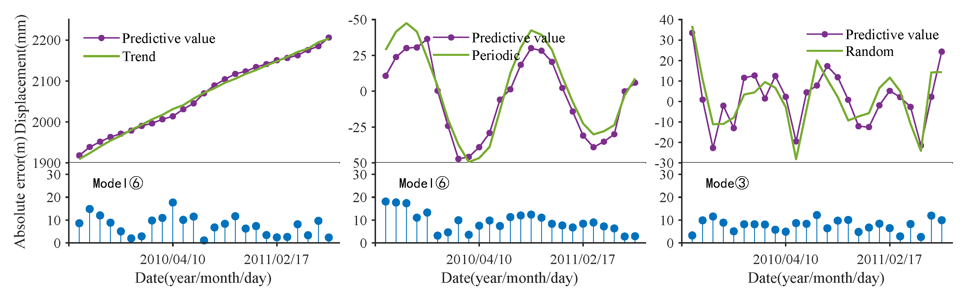
4.2.1. Displacement Components Prediction

The DES is employed to predict the trend component of the landslide displacement by using a weighted combination of past observations with recent observations given relatively higher weights than the older ones. Thus, despite the data volume difference between the designed six training datasets, the predicted trend component displacement is almost identical. Here, the prediction of Model 6 is taken as the final trend result. The DES results and the absolute error are shown in Figure 12a, with R² = 0.998 and RMSE = 2.741 mm.

The GRU could adaptively capture dependencies at different time scales, especially suitable for handling non-linear problems, and is thus used to forecast landslide displacements for periodic and random terms. The performance of the GRU in predicting the periodic component of the landslide displacement is shown in

Table 3. The performance of the GRU in predicting periodic and random displacement.

Model Number	ZG93
	Periodic		Random
	RMSE (mm)	R2	RMSE (mm)	R2
1	21.562	0.503	9.647	0.507
2	20.722	0.541	8.729	0.597
3	18.741	0.624	8.127	0.651
4	14.042	0.789	9.107	0.569
5	11.171	0.867	9.196	0.552
6	10.175	0.889	9.468	0.514

. According to Table 3, the GRU performance increases as the training data volume increases; thus, the optimal result is achieved with Model 6. However, the model performance of the random component displacement first increases and then decreases; the optimal results come from Model 3.

The above results indicate that better periodic component prediction needs more trained data; of the six designed models, the larger the amount of the training data, the better. However, it does not apply to random components; for random component forecasts, an appropriate amount of datasets works best.

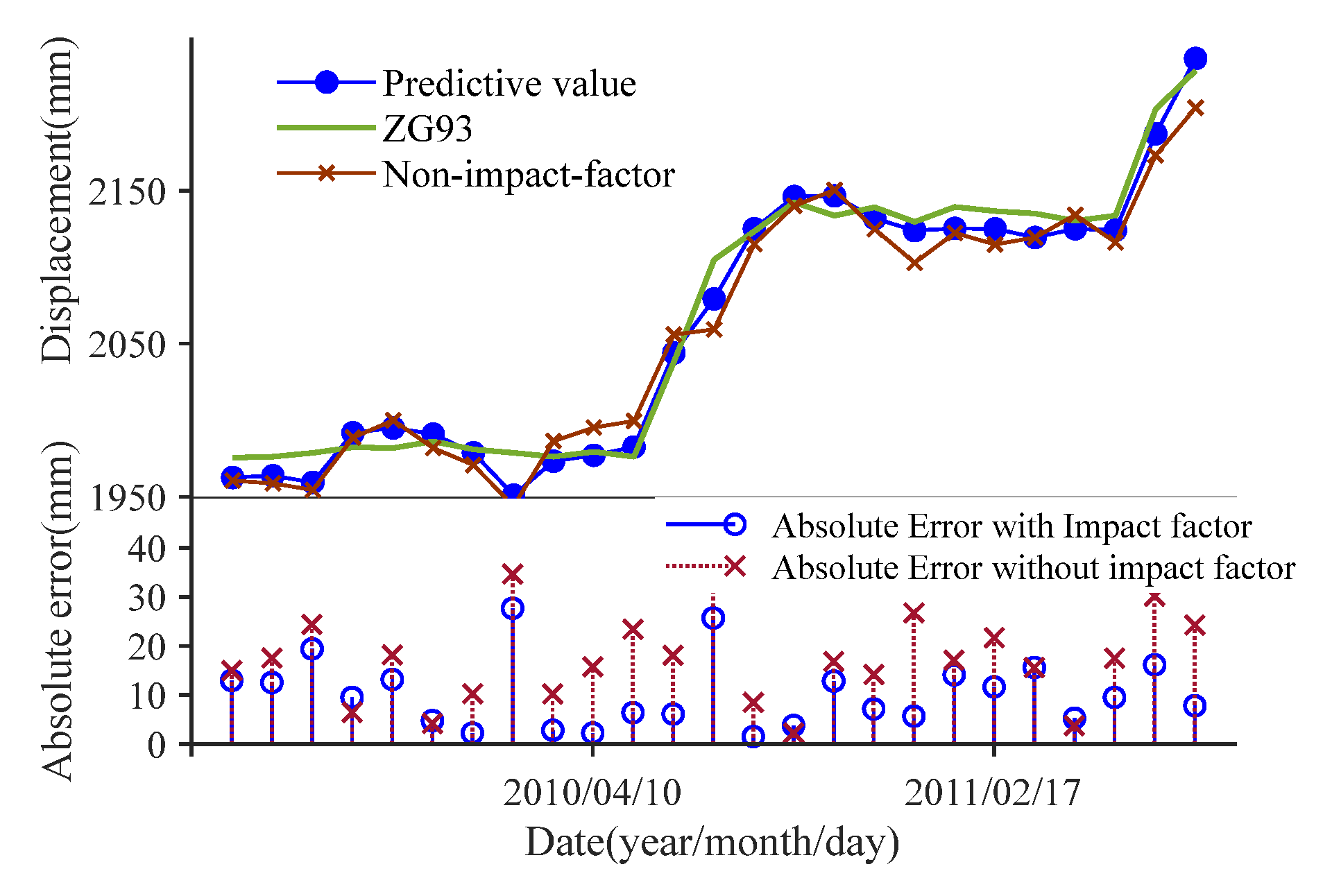
4.2.2. Cumulative Displacement Prediction

The predicted cumulative displacements can be derived by combining the trend, the periodic and the random predicted components. The optimal prediction of each component is illustrated in Figure 12. According to Figure 12, the absolute forecast error of the trend component remains small (<20 mm) and does not vary much, despite the deformation being around 2 m. In contrast, the absolute forecast error of the periodic component follows a certain regularity and shows a tendency to decrease, and that of the random component shows randomness.

The evaluation indicators, as listed in

Table 4. Predictions of the cumulative landslide displacement.

Model Number	ZG93
	RMSE (mm)	R2
1	24.165	0.917
2	26.043	0.904
3	20.367	0.941
4	18.582	0.952
5	20.106	0.943
6	18.742	0.951
Optimal model	12.301	0.979

, assess the performance of the six models. According to Table 4, both indicators experience an increase and then a decrease as the volume of the training dataset increases. A maximum RMSE of 26.043 mm and a minimum R² of 0.904 comes from Model 2 with a data volume of two natural years. The turning point found at Model 4 with four years of data volume shows the best results among the six models, with R² of 0.952 and RMSE of 18.582 mm.

According to Section 4.2.1, Model 6 is the best model for predicting the periodic component, while Model 3 gives the best performance for predicting the random part. Consequently, based on this, an optimal combination prediction model for landslide displacement is constructed. The evaluation indicators of the optimal model, shown in Table 4, outperform the other six models in terms of both evaluation indicators, with an RMSE of 12.301 mm and R² of 0.979. Compared with Model 4, the best forecast model among the six, the RMSE decreases by 6.281 mm and R² increases by 0.027 for the optimal model.

4.2.3. Comparative Experiments and Analyses

In Section 3.2, we conducted a pre-selection of the impact factors, and later, through the multi-scale response analysis in Section 3.3, we gained valuable insights into how the landslide responds to the dynamic interplay of the selected factors. The analysis revealed an apparent 1 year primary cycle of the time series associated with the landslide evolution. Of particular interest were the delayed response results, which highlight the complex interactions between the reservoir water level (R.w.l) and rainfall with the subsequent landslide movements. This provides a deeper understanding of the landslide’s complex behavior and guides the selection of the landslide prediction model.

GRU and other recurrent neural networks (RNNs) excel at handling the non-linear dynamic characteristics present in complex time series. The GRU model, in particular, has the ability to capture dependencies at different time scales, making it well-suited for time series landslide displacement prediction. Considering the outstanding performance of GRU in time-series forecasting, we conducted comparative experiments to analyze the performance differences of the optimal model screened in Section 4.2.2, both when considering impact factors and when not considering them.

Figure 13 displays the predicted cumulative displacements and absolute errors. Notably, when the impact factors are ignored, the model exhibits more significant deviations, indicating a decline in prediction performance. The calculated RMSE and R² are 20.218 mm and 0.942, respectively. However, when considering the impact factors, the model produces an improved performance, yielding an RMSE of 12.301 mm and R² of 0.979. This results in a reduction in the RMSE by 7.917 mm and an increase in R2 by 0.037, respectively.

As a result, the impact factors selected in Section 3.2 have been proven to be indispensable for multi-scale response analysis and the prediction model training process. Despite the exceptional performance of GRU in time-series forecasting, it is evident that the influence factors of landslides displacement have a significant impact on the predictions. Hence, the analysis and selection of the impact factors during the modeling process are crucial, underscoring the comprehensiveness of the proposed model.

At this stage, the 17 reserved sets of data from August 2011 to December 2012 are utilized for model validation to further verify the model’s performance. Figure 14 displays the cumulative landslide displacement prediction (17 sets) and the absolute errors of the proposed model, resulting in a calculated RMSE of 9.715 mm and R² of 0.967. The results demonstrate that the optimal combination prediction model exhibits a reliable capacity for predicting landslide displacement.

To further illustrate the superiority of the proposed method compared to existing state-of-the-art methods, such as the GWO-MIC-SVR [42], the V/S-LSTM [43], the Chaotic DWT-ELM [44] and the Multi-Chaotic ELM [45], we conduct a comparative analysis of the forecasts generated by these models. The performance of the forecast models is shown in

Table 5. Comparison of model prediction results.

Model Name	Forecast Duration (month)	RMSE (mm)
The method proposed	17	9.715
PSO-SVR	12	20.770
GWO-MIC-SVR	18	14.024
M-EEMD-ELM	15	-
V/S-LSTM	8	8.950
Chaotic DWT-ELM	15	23.330
Multi-Chaotic ELM	20	23.710

.

According to Table 5, the proposed model achieves a competitive high-accuracy result in terms of RMSE, ranking in the top two, with an RMSE of 9.715 mm, closely following the V/S-LSTM with an RMSE of 8.950 mm. However, what makes the proposed model stands out is its ability to makes 17 sets of consecutive forecasts, while V/S-LSTM only forecasts 8 sets.

Considering that forecast errors can accumulate over time, the proposed model’s RMSE of 0.765 mm for 17 sets of consecutive forecasts demonstrates its capability for precise and reliable long-term predictions. Thus, from a comprehensive perspective, the proposed model exhibits both time-effectiveness and long-sequence forecasting advantages over the other six intelligent algorithms.

5. Conclusions

This paper presents a novel deep learning architecture specifically designed for predicting reservoir landslide displacement. The evolution of reservoir landslides involves highly complicated and nonlinear dynamics, characterized by specific time-frequency features. To address the complexities, the joint time-frequency analysis (JTFA) module is designed. This module integrates the GWO-optimized VMD and WA methods, facilitating the extraction of essential signal components with clear physical implications. Additionally, the module conducts multi-scale response analysis, thereby revealing deformation variation patterns in the underlying mechanisms governing the landslide’s response behavior. For the actual displacement prediction, The GRU is integrated, which possesses the capability of adaptively capturing dependencies at multiple time scales. Moreover, during the modeling process, the correlation and hysteresis effect of the impact factors are also considered, further enhancing the accuracy and reliability of the predictions. The model experiments show that as the amount of training data increases, the periodic component prediction improves significantly. For the random component forecast, an appropriate amount of datasets yields the best results, while the trend component remains almost identical regardless of the data size. This insight led to the construction of an optimal combination prediction model, surpassing the performance of the other six designed models in cumulative landslide displacement predictions. This model achieved impressive results, with a minimum RMSE of 12.301 mm and a maximum R2 of 0.979. Moreover, the proposed architecture’s superiority in time-effectiveness and its ability to accurately predict long-sequence landslide displacement have been firmly established through comparative experiments and analyses, in which we evaluated its performance against six other state-of-the-art intelligent methods. The favorable outcomes and impressive forecasting capabilities of our proposed architecture solidify its position as an efficient and accurate tool for landslide displacement prediction.

References

1. Yin, Y.; Huang, B.; Wang, W.; Wei, Y.; Ma, X.; Ma, F.; Zhao, C. Reservoir-Induced Landslides and Risk Control in Three Gorges Project on Yangtze River, China. J. Rock Mech. Geotech. Eng. 2016, 8, 577–595. [Google Scholar] [CrossRef] [Green Version]
2. Zhou, C.; Yin, K.; Cao, Y.; Ahmed, B. Application of Time Series Analysis and PSO–SVM Model in Predicting the Bazimen Landslide in the Three Gorges Reservoir, China. Eng. Geol. 2016, 204, 108–120. [Google Scholar] [CrossRef]
3. Tang, H.; Wasowski, J.; Juang, C.H. Geohazards in the Three Gorges Reservoir Area, China–Lessons Learned from Decades of Research. Eng. Geol. 2019, 261, 105267. [Google Scholar] [CrossRef]
4. Wang, F.; Li, T. (Eds.) Landslide Disaster Mitigation in Three Gorges Reservoir, China; Environmental Science and Engineering; Springer: Berlin/Heidelberg, Germany, 2009; ISBN 978-3-642-00131-4. [Google Scholar]
5. Wang, F.-W.; Zhang, Y.-M.; Huo, Z.-T.; Matsumoto, T.; Huang, B.-L. The July 14, 2003 Qianjiangping Landslide, Three Gorges Reservoir, China. Landslides 2004, 1, 157–162. [Google Scholar] [CrossRef]
6. Schulte, J.A. Wavelet Analysis for Non-Stationary, Nonlinear Time Series. Nonlin. Process. Geophys. 2016, 23, 257–267. [Google Scholar] [CrossRef] [Green Version]
7. Rhif, M.; Ben Abbes, A.; Farah, I.R.; Martínez, B.; Sang, Y. Wavelet Transform Application for/in Non-Stationary Time-Series Analysis: A Review. Appl. Sci. 2019, 9, 1345. [Google Scholar] [CrossRef] [Green Version]
8. Huang, F.; Huang, J.; Jiang, S.; Zhou, C. Landslide Displacement Prediction Based on Multivariate Chaotic Model and Extreme Learning Machine. Eng. Geol. 2017, 218, 173–186. [Google Scholar] [CrossRef]
9. Jiang, Y.; Xu, Q.; Lu, Z.; Luo, H.; Liao, L.; Dong, X. Modelling and Predicting Landslide Displacements and Uncertainties by Multiple Machine-Learning Algorithms: Application to Baishuihe Landslide in Three Gorges Reservoir, China. Geomat. Nat. Hazards Risk 2021, 12, 741–762. [Google Scholar] [CrossRef]
10. Zhang, W.; Li, H.; Tang, L.; Gu, X.; Wang, L.; Wang, L. Displacement Prediction of Jiuxianping Landslide Using Gated Recurrent Unit (GRU) Networks. Acta Geotech. 2022, 17, 1367–1382. [Google Scholar] [CrossRef]
11. He, B.; Chang, J.; Wang, Y.; Wang, Y.; Zhou, S.; Chen, C. Spatio-Temporal Evolution and Non-Stationary Characteristics of Meteorological Drought in Inland Arid Areas. Ecol. Indic. 2021, 126, 107644. [Google Scholar] [CrossRef]
12. Su, L.; Miao, C.; Duan, Q.; Lei, X.; Li, H. Multiple-Wavelet Coherence of World’s Large Rivers with Meteorological Factors and Ocean Signals. J. Geophys. Res. Atmos. 2019, 124, 4932–4954. [Google Scholar] [CrossRef]
13. Huang, N.E.; Shen, Z.; Long, S.R.; Wu, M.C.; Shih, H.H.; Zheng, Q.; Yen, N.-C.; Tung, C.C.; Liu, H.H. The Empirical Mode Decomposition and the Hilbert Spectrum for Nonlinear and Non-Stationary Time Series Analysis. Proc. R. Soc. Lond. A 1998, 454, 903–995. [Google Scholar] [CrossRef]
14. Dragomiretskiy, K.; Zosso, D. Variational Mode Decomposition. IEEE Trans. Signal Process. 2014, 62, 531–544. [Google Scholar] [CrossRef]
15. Isham, M.F.; Leong, M.S.; Lim, M.H.; Ahmad, Z.A. Variational Mode Decomposition: Mode Determination Method for Rotating Machinery Diagnosis. J. Vibroengineering 2018, 20, 2604–2621. [Google Scholar] [CrossRef] [Green Version]
16. Haghshenas, S.S.; Haghshenas, S.S.; Geem, Z.W.; Kim, T.-H.; Mikaeil, R.; Pugliese, L.; Troncone, A. Application of Harmony Search Algorithm to Slope Stability Analysis. Land 2021, 10, 1250. [Google Scholar] [CrossRef]
17. Mirjalili, S.; Mirjalili, S.M.; Lewis, A. Grey Wolf Optimizer. Adv. Eng. Softw. 2014, 69, 46–61. [Google Scholar] [CrossRef] [Green Version]
18. Fang, K.; Tang, H.; Li, C.; Su, X.; An, P.; Sun, S. Centrifuge Modelling of Landslides and Landslide Hazard Mitigation: A Review. Geosci. Front. 2023, 14, 101493. [Google Scholar] [CrossRef]
19. Olsen, J.; Anderson, N.J.; Knudsen, M.F. Variability of the North Atlantic Oscillation over the Past 5200 Years. Nat. Geosci 2012, 5, 808–812. [Google Scholar] [CrossRef]
20. Gan, T.Y.; Gobena, A.K.; Wang, Q. Precipitation of Southwestern Canada: Wavelet, Scaling, Multifractal Analysis, and Teleconnection to Climate Anomalies. J. Geophys. Res. Atmos. 2007, 112, D10110. [Google Scholar] [CrossRef]
21. Torrence, C.; Webster, P.J. Interdecadal Changes in the ENSO–Monsoon System. J. Clim. 1999, 12, 2679–2690. [Google Scholar] [CrossRef]
22. Torrence, C.; Compo, G.P. A Practical Guide to Wavelet Analysis. Bull. Amer. Meteor. Soc. 1998, 79, 61–78. [Google Scholar] [CrossRef]
23. Grinsted, A.; Moore, J.C.; Jevrejeva, S. Application of the Cross Wavelet Transform and Wavelet Coherence to Geophysical Time Series. Nonlin. Process. Geophys. 2004, 11, 561–566. [Google Scholar] [CrossRef]
24. Tomás, R.; Li, Z.; Lopez-Sanchez, J.M.; Liu, P.; Singleton, A. Using Wavelet Tools to Analyse Seasonal Variations from InSAR Time-Series Data: A Case Study of the Huangtupo Landslide. Landslides 2016, 13, 437–450. [Google Scholar] [CrossRef] [Green Version]
25. Hu, X.; Wu, S.; Zhang, G.; Zheng, W.; Liu, C.; He, C.; Liu, Z.; Guo, X.; Zhang, H. Landslide Displacement Prediction Using Kinematics-Based Random Forests Method: A Case Study in Jinping Reservoir Area, China. Eng. Geol. 2021, 283, 105975. [Google Scholar] [CrossRef]
26. Fang, K.; Dong, A.; Tang, H.; An, P.; Zhang, B.; Miao, M.; Ding, B.; Hu, X. Comprehensive Assessment of the Performance of a Multismartphone Measurement System for Landslide Model Test. Landslides 2023, 20, 845–864. [Google Scholar] [CrossRef]
27. Jiang, Y.; Luo, H.; Xu, Q.; Lu, Z.; Liao, L.; Li, H.; Hao, L. A Graph Convolutional Incorporating GRU Network for Landslide Displacement Forecasting Based on Spatiotemporal Analysis of GNSS Observations. Remote Sens. 2022, 14, 1016. [Google Scholar] [CrossRef]
28. Zhang, X.; Zhu, C.; He, M.; Dong, M.; Zhang, G.; Zhang, F. Failure Mechanism and Long Short-Term Memory Neural Network Model for Landslide Risk Prediction. Remote Sens. 2022, 14, 166. [Google Scholar] [CrossRef]
29. Chung, J.; Gulcehre, C.; Cho, K.; Bengio, Y. Empirical Evaluation of Gated Recurrent Neural Networks on Sequence Modeling. arXiv 2014, arXiv:1412.3555. [Google Scholar]
30. Wang, B.; Wang, J. Energy Futures and Spots Prices Forecasting by Hybrid SW-GRU with EMD and Error Evaluation. Energy Econ. 2020, 90, 104827. [Google Scholar] [CrossRef]
31. Gao, S.; Huang, Y.; Zhang, S.; Han, J.; Wang, G.; Zhang, M.; Lin, Q. Short-Term Runoff Prediction with GRU and LSTM Networks without Requiring Time Step Optimization during Sample Generation. J. Hydrol. 2020, 589, 125188. [Google Scholar] [CrossRef]
32. Shannon, C.E. A Mathematical Theory of Communication. Mob. Comput. Commun. Rev. 1997, 5, 53. [Google Scholar]
33. Kingma, D.P.; Ba, J. Adam: A Method for Stochastic Optimization. arXiv 2017, arXiv:1412.6980. [Google Scholar]
34. Zhu, X.; Xu, Q.; Tang, M.; Li, H.; Liu, F. A Hybrid Machine Learning and Computing Model for Forecasting Displacement of Multifactor-Induced Landslides. Neural Comput. Appl. 2018, 30, 3825–3835. [Google Scholar] [CrossRef]
35. Lian, C.; Zeng, Z.; Yao, W.; Tang, H. Multiple Neural Networks Switched Prediction for Landslide Displacement. Eng. Geol. 2015, 186, 91–99. [Google Scholar] [CrossRef]
36. Li, X.; Zhang, N.X.; Liao, Q.L.; Wu, J. Analysis on Hydrodynamic Field Influenced by Combination of Rainfall and Reservoir Level Fluctuation. Chin. J. Rock Mech. Eng. 2004, 23, 3714–3720. [Google Scholar]
37. Yang, B.; Yin, K.; Lacasse, S.; Liu, Z. Time Series Analysis and Long Short-Term Memory Neural Network to Predict Landslide Displacement. Landslides 2019, 16, 677–694. [Google Scholar] [CrossRef]
38. Wu, Q.; Tang, H.M.; Wang, L.Q.; Lin, Z.H. Analytic Solutions for Phreatic Line in Reservoir Slope with Inclined Impervious Bed under Rainfall and Reservoir Water Level Fluctuation. Rock Soil Mech. 2009, 30, 3025–3031. [Google Scholar]
39. Guo, Z.; Chen, L.; Gui, L.; Du, J.; Yin, K.; Do, H.M. Landslide Displacement Prediction Based on Variational Mode Decomposition and WA-GWO-BP Model. Landslides 2020, 17, 567–583. [Google Scholar] [CrossRef]
40. Fang, Z.; Hang, D.; Xinyi, Z. Rainfall Regime in Three Gorges Area in China and the Control Factors: Rainfall regime in three gorges area in china. Int. J. Climatol. 2010, 30, 1396–1406. [Google Scholar] [CrossRef]
41. Yao, Y.; Luo, Y.; Zhang, J.; Zhao, C. Correlation Analysis between Haze and GNSS Tropospheric Delay Based on Coherent Wavelet. Geomat. Inf. Sci. Wuhan Univ. 2018, 43, 2131–2138. [Google Scholar]
42. Li, L.; Wu, Y.; Miao, F.; Liao, K.; Zhang, L. Displacement Prediction of Landslides Based on Variational Mode Decomposition and GWO-MIC-SVR Model. Chin. J. Rock Mech. Eng. 2018, 37, 1395–1406. [Google Scholar]
43. Feng, F.; Wu, X.; Niu, R.; Xu, S. A Landslide Deformation Analysis Method Using V/S and LSTM. Landslide Deform. Anal. Method. 2019, 44, 784–790. [Google Scholar]
44. Huang, F.; Yin, K.; Zhang, G.; Gui, L.; Yang, B.; Liu, L. Landslide Displacement Prediction Using Discrete Wavelet Transform and Extreme Learning Machine Based on Chaos Theory. Env. Earth Sci. 2016, 75, 1376. [Google Scholar] [CrossRef]
45. Huang, F.; Yin, K.; Yang, B.; Li, X.; Liu, L.; Fu, X.; Li, X. Step-like Displacement Prediction of Landslide Based on Time Series Decomposition and Multivariate Chaotic Model. Earth Sci. 2018, 43, 887–898. [Google Scholar]
Figure 1. Architecture of the forecasting model.
Remotesensing 15 03995 g001
Figure 2. The network structure of GRU.
Remotesensing 15 03995 g002
Figure 3. (a) Location of the landslide. (b) monitoring layout diagram. (c) geological profile III through point ZG93.
Remotesensing 15 03995 g003
Figure 4. Monitoring data in time series of the Baishuihe landslide.
Remotesensing 15 03995 g004
Figure 5. Decomposition result of displacement at ZG93.
Remotesensing 15 03995 g005
Figure 6. Rainfall effects on landslide displacement.
Remotesensing 15 03995 g006
Figure 7. Relations between the periodical deformation and the reservoir level fluctuation.
Remotesensing 15 03995 g007
Figure 8. Decomposition results of the six influence factors (V1V6), with the subscript p indicates the periodic term and subscript s indicates the random term.
Remotesensing 15 03995 g008
Figure 9. The CWT power spectrum of the rainfall (a), the reservoir water level (R.w.l) (b) and the displacement at ZG93 (c). Regions enclosed by the heavy solid black line show a greater than 95% confidence level of the red noise standard spectrum. The cross-hatched regions on either end indicate the “cone of influence”, where edge effects become important. Color changes mean different magnitudes of power.
Remotesensing 15 03995 g009
Figure 10. The XWT power and WTC coherence spectrum of R.w.l and rainfall. The arrow direction reflects the phase correlation between the two time series. The arrow points from left to right indicate the in-phase relation, and the opposite suggests the anti-phase. In XWT, the color change indicates the magnitude of power. In WTC, the color differences suggest different magnitudes of coherence.
Remotesensing 15 03995 g010
Figure 11. The XWT power and WTC coherence spectrum of the periodic term and six impact factors. (a,b) indicate rainfall-type factors V2 and V3. The remainder indicates reservoir-type factors, where (cf) indicate monthly mean level V1, monthly variation V4, single-month rate of change V5 and bi-monthly variation V6.
Remotesensing 15 03995 g011
Figure 12. Predictions of each displacement component.
Remotesensing 15 03995 g012
Figure 13. Predictions of the cumulative landslide displacement. The red marker indicates the absolute error without considering influencing factors, while the blue circle indicates the absolute error of our proposed method.
Remotesensing 15 03995 g013
Figure 14. Predictions of the cumulative landslide displacement. The blue circles stands for the absolute errors of the proposed model.
Remotesensing 15 03995 g014