Article

Improved Object-Based Mapping of Aboveground Biomass Using Geographic Stratification with GEDI Data and Multi-Sensor Imagery

1
Institute of Remote Sensing and Earth Sciences, School of Information Science and Technology, Zhejiang Provincial Key Laboratory of Urban Wetlands and Regional Change, Hangzhou Normal University, Hangzhou 311121, China
2
Key Laboratory of Wetland Ecology and Environment, Northeast Institute of Geography and Agroecology, Chinese Academy of Sciences, Changchun 130102, China
3
Fujian Key Laboratory of Big Data Application and Intellectualization for Tea Industry, Wuyi University, Wuyishan 354300, China
4
National Earth System Science Data Center, Beijing 100101, China
5
Hebei Key Laboratory of Mining Development and Security Technology, Hebei Industrial Technology Institute of Mine Ecological Remediation, College of Mining Engineering, North China University of Science and Technology, Tangshan 063210, China
*
Author to whom correspondence should be addressed.
Remote Sens. 2023, 15(10), 2625; https://doi.org/10.3390/rs15102625
Submission received: 27 March 2023 / Revised: 15 May 2023 / Accepted: 16 May 2023 / Published: 18 May 2023

Abstract

:
Aboveground biomass (AGB) mapping using spaceborne LiDAR data and multi-sensor images is essential for efficient carbon monitoring and climate change mitigation actions in heterogeneous forests. The optimal predictors of remote sensing-based AGB vary greatly with geographic stratification, such as topography and forest type, while the way in which geographic stratification influences the contributions of predictor variables in object-based AGB mapping is insufficiently studied. To address the improvement of mapping forest AGB by geographic stratification in heterogeneous forests, satellite multisensory data from global ecosystem dynamics investigation (GEDI) and series of advanced land observing satellite (ALOS) and Sentinel were integrated. Multi-sensor predictors for the AGB modeling of different types of forests were selected using a correlation analysis of variables calculated from topographically stratified objects. Random forests models were built with GEDI-based AGB and geographically stratified predictors to acquire wall-to-wall biomass values. It was illustrated that the mapped biomass had a similar distribution and was approximate to the sampled forest AGB. Through an accuracy comparison using independent validation samples, it was determined that the geographic stratification approach improved the accuracy by 34.79% compared to the unstratified process. Stratification of forest type further increased the mapped AGB accuracy compared to that of topography. Topographical stratification greatly influenced the predictors’ contributions to AGB mapping in mixed broadleaf–conifer and broad-leaved forests, but only slightly impacted coniferous forests. Optical variables were predominant for deciduous forests, while for evergreen forests, SAR indices outweighed the other predictors. As a pioneering estimation of forest AGB with geographic stratification using satellite multisensory data, this study offers optimal predictors and an advanced method for obtaining carbon maps in heterogeneous regional landscapes.

Graphical Abstract

1. Introduction

Forest biomass serves as an essential factor in determining the status of ecosystem functions and terrestrial carbon stock [1]. Regional wall-to-wall estimations of forest aboveground biomass (AGB) are in great demand for the rational utilization of forest resources and alleviating climate change [2,3]. Consequently, decreasing the uncertainty and upgrading the efficiency of precise forest AGB mapping is an urgent matter.
Satellite remote sensors for monitoring forests in an efficient and spatiotemporally consistent way have become a fundamental technology for wall-to-wall AGB estimation [4]. Passive or active remote sensing techniques exhibit both strengths and weaknesses in retrieving forest AGB; reflectance and spectral indices from optical sensors are sensitive to the chlorophyll content and horizontal structure of vegetation cover, but are subject to climate and saturation problems [5]. Backscatters with different polarization and penetrability from radar sensors, especially from SAR, directly relate to AGB in water-cloud models [6,7]. Moreover, topographic indices from interferometric SAR (InSAR), on behalf of the local hydrothermal condition, are conventional variables for forest AGB prediction. However, fine-resolution satellite radar images are relatively inaccessible and still suffer from signal saturation in heterogeneous forests with a biomass above 150 Mg/ha [8,9]. LiDAR has earned a reputation for excellent penetrability into dense canopy cover and provides three-dimensional structure features to facilitate biomass prediction [10,11]. Because of the coverage, LiDAR variables are conventionally integrated with optical and radar images [12,13]. Satellite GEDI LiDAR with assistance from series of Sentinel and ALOS has become the primary efficient, spatiotemporally uniform method for AGB estimation, owing to its open-access global coverage and finer spatiotemporal resolution [14,15].
A point–line–polygon framework is generally constructed to achieve the above-mentioned integration of spaceborne footprint LiDAR signals and images to yield accurate biomass maps [16]. Indeed, field-measured AGB points calculated from ground samples are predicted by LiDAR variables. Polygon-level biomass prediction is then conventionally modeled based on a pixel-size relationship between the LiDAR AGB lines and predictors from multi-sensor images [12,17]. In other words, the values of multi-sensor variables and predicted AGB are the exact values within the pixel. Meanwhile, LiDAR-estimated AGB lines are subsequently modeled by predictor variables from SAR and optical imagery based on an object’s size for lessening uncertainty in the positional discrepancy and local heterogeneity [17]. Different from the pixel-based approach, multi-sensor variable values are calculated as the mean values within optimal objects during object-based mapping, and the final modeling unit is also the object. This modeling is commonly conducted using machine learning methods, due to the complex nonlinear relationships between remote sensing indices and forest AGB [1,12]. In contrast, AGB estimations of heterogeneous forests are still a massive challenge due to the uncertainty that results from significant variation in optimal predictors with geographic stratification such as topography and forest type [18,19]. In spite of a few studies on the influence of geographic stratification on pixel-based AGB mapping, how geographic stratification influences the uncertainty of object-based AGB mapping deserves further exploration. Hence, the comparative development of geographic stratification with the unstratified approach enables precise object-based AGB mapping.
Aiming to facilitate full-cover forest AGB estimation, this study established geographically stratified object-based mapping using satellite data from LiDAR, SAR and MSI. Specific objectives were targeted: (1) quantifying the connections between forest AGB and multi-sensor variables using geographical stratification or an unstratified process by optimal predictors and attribute importance; (2) contrastively analyzing geographically stratified and unstratified object-based estimation by modeling comparison; (3) mapping heterogeneous forest AGB by geographical stratification.

2. Materials and Methods

2.1. The Study Area

As part of the Changbai Mountains mixed forests ecoregion within eastern Jilin Province in Northeast China, this heterogeneous mountainous area includes eight forest farms and covers 54,040.79 ha of forests (Figure 1). It has a monsoon-affected moist continental climate with four distinct seasons. This area’s distribution is mainly deciduous broad-leaved forest (82.59%) and mixed broadleaf–conifer forest (11.61%). The typical regional species are Quercus mongolica Fisch. ex Ledeb. and Betula platyphylla Suk. for the deciduous broad-leaved forests, Pinus koraiensis Siebold et Zuccarini for the evergreen coniferous forests, Larix gmelinii (Rupr.) Kuzen for the deciduous coniferous forests, and Betula and Picea asperata Mast. for the mixed broadleaf–conifer forests.

2.2. Data

2.2.1. Ground-Sampled Measurements

The forest type map was provided by the local forestry bureau in a vector format, as shown in Figure 1a. The sampling sites, randomly covering forest areas, were generated in the lab. Then, the field campaign across the study area began in May 2019 and continued for four months, with unavailable samples being substituted by the nearest homogeneous plots for the measurements. Then, 1111 samples with a square of approximately 25 m on one side were observed (Figure 1a), including 826, 143, 116, and 26 plots in deciduous broad-leaved, mixed broadleaf–conifer, deciduous coniferous, and evergreen coniferous forests, respectively. Calculating from the measured diameter at breast height and tree height and from allometric equations (Table 1), the values of field-based AGB were the sum of the trunks, branches and leaves.

2.2.2. Pre-Processing of Multi-Sensor Data

The canopy cover and height from spaceborne LiDAR signals have been widely verified in previous research, which generalized linearly related to AGB [21,22]. The GEDI level 2B canopy cover and vertical profile metrics product (GEDI L2B) was derived from each original waveform based on the directional gap probability profile, which provided accurate location, height, and canopy cover data. Using the rGEDI R Package [23], the canopy cover and height were extracted from downloaded GEDI L2B data from the NASA Earthdata Search as reported in Table 2, spatiotemporally in line with the field campaign. Then, 15,893 valid pairs of canopy cover and height were obtained (Figure 1b and Figure 2).
A total of 891 training points contained in the valid pairs were chosen from the 1111 field-measured AGB samples for the biomass modeling. The remaining 220 samples served as validation points for comparing the model performance (Figure 1).
The adopted multi-sensor images are as shown in Table 2. All mosaic images were pretreated with topographical correction and obtained using the Google Earth Engine (GEE) platform [24]. Specifically, an ALOS-2 yearly mosaic image in 2019 (Figure 1c) was selected, masked, and transformed to a normalized backscatter coefficient [25]. The Sentinel-1 mosaic (Figure 1d) was produced from 40 images at a ground-range-detected level from May to September 2019 using Lee filtering, masking, converting and mosaicking [24]. The S2 mosaic was composited after the disposal of cloud and noise, as the median of multispectral bands from 61 Sentinel-2A L2A images (Figure 1e). The ALOS-1 DSM products were downloaded from the GEE (Figure 1f) for calculations of topographic indicators (Figure 2). After that, the preprocessed images were converted to the same projection and spatial resolution.
On the basis of the predictor variables in correlational research on AGB modeling [26,27], a total of 53 variables were elected, including 4, 24, 19, and 6 from A2, S1, S2, and DSM, respectively (Table 3). Taking advantage of the reflections of forest structures but insusceptibility to terrain, multi-frequency SAR-estimated normalized backscatter coefficients and their calculations, as well as texture features from S1, were generated from the mosaic images in SNAP software [28]. The reflectance and vegetation indices from the S2 mosaic, the commonly used variables for AGB modeling, were calculated [29,30]. Topographic indicators, as proxies of potential solar radiation and moisture distribution for the partial explanation of spatial patterns in AGB, were extracted from DSM [31].

2.3. Methods

For enhancing forest AGB mapping with geographic stratification, the methodology comprised three main elements (Figure 2). The improvement was quantified with an accuracy comparison among four models, i.e., the stratification of geography, topography, forest type, and the unstratified process. Indeed, these models’ processes were different, as were the units of variable calculation and AGB prediction.
The geographically stratified mapping included two-step stratification of topography and forest type: (1) the variable calculated as an average in each object was segmented from DSM and S2, which was defined as a step of topographical stratification, and the prediction unit was also this object; (2) predictor selection and AGB modeling were conducted separately among deciduous broad-leaved, evergreen coniferous, deciduous coniferous, and mixed broadleaf–conifer forests, which was a step of stratification by forest type. The final geographically stratified prediction was the mosaic of four AGB maps from four forest types. In unstratified mapping, the variables’ values and predicted AGB were the mean values inside each object segmented only from S2, and the predictor selection and modeling were based on the whole forests.

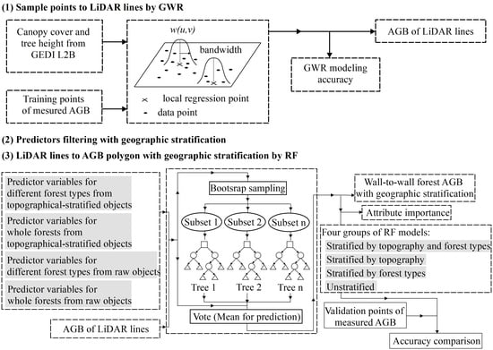
2.3.1. GWR Modeling for GEDI-Derived AGB Lines

The substantial literature indicated the potential for AGB estimations based on solving generalized linear models and spaceborne LiDAR-derived canopy cover and height [32,33], but their relationships change according to the location. Therefore, geographically weighted regression (GWR) was adopted in this study, as shown in Figure 3 [34]. As an extension of orthogonal least squares, the GWR incorporated geographic information into GEDI-based AGB modeling, with individual calculation of the local parameters that followed the distance attenuation [35,36]. GWR4 software was used to establish a GWR model to estimate GEDI-based AGB by quantifying parameters, such as the types of model and kernel, as well as the method and criteria of bandwidth selection [37].

2.3.2. Filtering Predictors for Different Forest Types from Topographically Stratified Objects

The object-based approach, minimizing positional discrepancy and local heterogeneity issues, was adopted to acquire variable values and conduct forest AGB mapping [16]. The object was conventionally obtained based on optical images [17,38], which was used as a comparison in this study, i.e., non-topographical stratification (Figure 2). For acquiring the object in the topographical stratification, multiresolution segmentation was performed on images combining S2 and DSM by assigning 0.1, 0.5, and 25 to the shape, compactness, and scale, respectively, with eCognition software. The conventional objects from a segmented S2 mosaic image, as a non-topographical stratification, were also obtained by setting the same parameter values. Then, the variable calculation was the mean inside an object linked to an AGB plot.
The predictor variables of AGB object-based mapping were determined using correlation analysis. The candidate was chosen from the significantly related variables (p < 0.05). Due to the influence of redundancy on the prediction precision of random forests (RF), the candidate’s collinearity was disposed (r ≥ 0.8), and the predictors were the most related [39,40].

2.3.3. Prediction Stratified or Raw AGB Polygons by RF

Owing to its lower sensitivity to the noise of training samples, RF is extensively employed in remote sensing-based AGB mapping and exhibits higher precision through the contrastive analysis [41,42]. Four groups of object-based RF models were built after setting the number of features and trees, and the variable importance was identified according to the mean-variance decrease [43,44]. For an explicit comparison of the contributions of the predictor variables, the relative variable importance was calculated as Xi/Xmax, where “Xi” and “Xmax” were the mean variance of predictor i and the maximum values of all predictors in an RF model, respectively. The AGB value was predicted as the average of all trees (Figure 4). Then, the precision was compared using the root-mean-square error (RMSE), mean error (ME), coefficient of determination (R2), and the relative improvement (RI) from 220 independent validation points [45,46]. A final AGB map was drawn using object-based RF mapping with geographic stratification.

3. Results

3.1. GEDI LiDAR-Extracted AGB Lines Using GWR

The sampled AGB was 0.35–548.22 Mg/ha, and the majority were less than 200 Mg/ha (Figure 5a). To visually display the distribution similarity of the mapped results with the measured values, the sampled AGB was divided by five levels at an equal frequency. The average, median, and standard deviation (SD) values were 140.56, 126.93, and 83.76 Mg/ha, respectively (Figure 5b). Among the different forest types, the mean of the sampled AGB had a peak of 154.64 Mg/ha in the mixed broadleaf–conifer forests, and a low of 72.92 Mg/ha in deciduous coniferous forests.
The GEDI-derived canopy cover values were 0.001–0.99, and those of canopy height were 1.35–54.39 m (Table 4). Based on the 891 training samples, a GWR model was established with the GEDI-derived canopy cover and height using a Gaussian approach weighted by a fixed Gaussian kernel, which achieved a smaller RMSE value than adaptive bandwidth. The optimal bandwidth was 2.36, determined by the golden selection method and small sample bias corrected Akaike information criterion (AICc). The AGB lines from 15,893 spaceborne LiDAR pairs ranged from 4.51 to 544.90 Mg/ha (Table 4). The mid-value was 142.53 Mg/ha and the SD value was 38.22 Mg/ha.

3.2. Predictor Variables for Different Forest Types from Topographically Stratified Objects

In total, 10 groups of predictor variables were obtained for RF modeling, after filtering by significant relations to AGB and disposing the redundancy, marked as “Yes” in Table S1. Overall, the related MSI variables had the highest redundancy, followed by variables from C and L band SAR. The 26 predictors were filtered out, including four from A2, eight from S1, 11 from S2, and three from DSM. Among them, HH was extensively chosen by seven groups; then B2 and red-edge vegetation indices that red-edge bands were involved in; RVI, EVI, VV_VAR, and NP; finally, the topographical indices followed.
With the topographical stratification, 31 variables were significantly related to the sampled AGB; 13 predictors were selected, including two from L band SAR, three from C band SAR, five from MSI, and three from DSM. In the unstratified process, VV_MEA additionally correlated significantly with AGB, and the 14 chosen predictors were also different from the topographical stratification. In detail, VV_ENT was included in the topographically stratified process but was replaced by VV_MAX in the unstratified approach, and EVI was extra filtered out as predictors without topographical stratification.
As for the stratification by forest type, the predictors were separately selected as shown in Table S1. On the whole, in both the topographically stratified and unstratified processes, optical variables were in the majority in predicting the AGB of deciduous forests, while SAR variables were dominant for evergreen coniferous and mixed broadleaf–conifer forests. Topographical stratification primarily distinguished the relationships between the measured AGB and SAR variables for deciduous broad-leaved and mixed broadleaf–conifer forests. In detail, with the topographical stratification, A2 predictors at a coarser resolution were replaced by S1 variables. For deciduous broad-leaved forests, HH was significantly related to AGB without redundancy in the unstratified process, which was replaced by VV in the topographically stratified process. In addition, VV_MEA was a substitute predictor for RFDI in mixed broadleaf–conifer forests with topographical stratification.

3.3. RF Models for AGB Prediction

The number of randomly chosen attributes as numFeatures in Weka software was set as the default, i.e., the integer value of (log2 M + 1), with ”M“ as the attribute number [47]. The tree number as numTrees was 500 in all RF models.
The results of the relative attribute importance showed that among the 26 predictors of the 10 RF models, optical variables were prominent, among which RVI was the most impressive (Figure 6). For whole forests, the sensors sorted by attribute importance were MSI from S2, InSAR from DSM, C band SAR from S1, and L band SAR from A2. The top five predictors of RF modeling with topographical stratification were RVI, MCARI, H, B2 and A. The change that non-stratification brought was the addition of EVI, filtered out in the topographically stratified predictor selection. In deciduous broad-leaved forests, the modeling contributions of sensors differed from whole forests. Specifically, C band SAR from S1 had a greater impact on AGB modeling than InSAR from DSM, and the vast majority of MSI—which derived all top-five variables, i.e., MCARI, RVI, MTCI, EVI, and SAVI—were outstanding. Moreover, the overwhelming majority of the MSI variables were enhanced by topographical stratification, with all optical predictors obtaining higher importance than the variables from S1. As for evergreen coniferous forests, L band SAR was the most contributive, and the predictors ranked by the attribute importance were V_H_L, HH, and VV_COR. In deciduous coniferous forests, the order was RVI, B3 and MTCI for the topographically stratified AGB modeling, but S2REP, B3, MTCI and EVI for the unstratified RF model. For mixed broadleaf–conifer forests, the attribute importance was considerably different between the topographically stratified and unstratified AGB modeling. In the topographically stratified modeling, S2 was more critical than S1, DSM, and A2, consistent with the sensor sorting in deciduous broad-leaved forests. Nonetheless, without topographical stratification, the predictors from A2 had a greater influence than S2, DSM and S1.
Overall, the vegetation indices from S2 MSI, the texture features from VV backscatters, and elevation were the primary variables for forest AGB prediction. The topographical stratification increased the advantages of optical predictors, but required finer-resolution SAR variables. The predictor variables, as well as their importance, largely varied according to forest type.
Table 5 shows the model accuracy calculated from 220 validation samples. The ME and RMSE are also expressed as a percentage in order to contrastively evaluate the accuracy to related studies, after being divided by the mean value of the measured AGB. The absolute values of ME denoted that four groups of RF modeling underestimated forest AGB. The validation results also demonstrated that geographic stratification by topography and forest type improved the prediction accuracy compared to the unstratified approach (Figure 7). The geographically stratified prediction lowered the RMSE values by 34.79%.

3.4. Forest AGB Map Predicted by Geographic Stratification

The forest AGB was illustrated using geographically stratified RF models (Figure 8a) and symbolized the same as the sampled AGB (Figure 5a). Generally, the mapped AGB had a similar value distribution to the measured biomass and was approximate to the observed values, described by the same pattern at each level. From the object-based RF model with multi-sensor data and geographical stratification, the mapped forest AGB ranged from 8.41 to 504.82 Mg/ha and had an average of 142.58 Mg/ha with an SD of 90.21 Mg/ha. The western and northern deciduous broad-leaved forests with a median elevation of 600–800 m had the largest AGB values, ranging from 190.58 to 504.82 Mg/ha. The deciduous coniferous forests with an altitude above 800 m exhibited the smallest AGB of 8.41–79.49 Mg/ha.

4. Discussion

4.1. Role of Topographical Stratification in AGB Estimation

The topographical stratification improved the prediction accuracy by modifying the objects of variable extraction and the AGB mapping (Figure 2). In other words, when the topographic variations are also taken into consideration, the segmented object as the basic unit can better relate predictors from multi-sensor images to AGB lines. The influence of the topographically stratified mapping was reflected in the selection of finer-resolution predictors and their contributions in mixed broadleaf–conifer and broad-leaved forests, but slightly impacted coniferous forests (Table S1). Indeed, the variables from the A2 predictors were replaced by the S1 variables, and the contributions of the S2 predictors were enhanced (Table S1 and Figure 6). The greater impact of topographical stratification on the AGB predictors of broad-leaved forests was possible because of more complex habitats, whereas conifer forests are chiefly located at higher altitudes with pure stands and simple structures [48]. In addition, selecting predictors with a finer resolution rather those with a stronger penetrability infers that vertical heterogeneity was reduced by topographical stratification, highlighting the horizontal variations in the broad-leaved forests. These relationships between forest type and topography are also called as the vertical zonality. In other words, the role of topographical stratification can be enhanced through application to other regions with distinguished vertical zonality.
The topographically stratified mapping was slightly more accurate than the unstratified prediction with an RIRMSE value of 3.40% (Table 5 and Figure 7). This implies that finer-resolution topographic data enhances the contribution. The precision of topographically stratified and unstratified mapping was less than the major regional maps of forest AGB, with RMSE values ranging from 21% to 67% [49], which may be explained by the benefits of multi-sensor integration and fine resolution. This is consistent with previous studies, which concluded that the integration of GEDI and series from ALOS and Sentinel was adequate for biomass mapping on a large scale [50].
In short, topographical stratification lowers vertical heterogeneity and is particularly essential for AGB mapping in broad-leaved forests. It should be emphasized that topographic data with higher spatiotemporal resolution are crucial for increasing the contribution of topographical stratification.

4.2. Influence of Stratification by Forest Type for AGB Estimation

Stratification by forest type increased the precision by separately selecting optimal predictors and building different RF models for the four forest types (Figure 2 and Table S1). Specifically, the optical variables from S2 MSI had closer relationships with AGB in broad-leaved forests, although the SAR indices had the most dominant response to forest biomass where evergreen trees were involved. This distinction is in agreement with the principle and characteristics of optical and SAR sensors. Optical remote sensing techniques retrieve AGB based on the typical reflectance of leaf chlorophyll, water content, and geometric structures [51]. Fittingly, the forest AGB of dense broad-leaved trees is closely linked to remote sensing-based canopy horizontal variables [52]. Nonetheless, the electromagnetic waves from SAR sensors interact with trunks and branches, generating particular indices as proxies of volume scattering and vertical information, which constitute the principal factors of AGB in evergreen forests [53]. The SAR predictors from A2 and S1 had different levels of importance among the forests. Namely, S1 was obviously more important than A2 in those forests where broad-leaved trees were involved. This can be explained by the coarser spatiotemporal resolution of A2 imagery and the horizontal variations discussed in Section 4.1. The independent validation showed that stratification by forest type vastly upgraded the precision of the unstratified model with an RIRMSE value of 24.4%. Simultaneously, this improvement was more considerable than the topographical stratification. Despite the above-mentioned coarse resolution of the topographic data, the independent validation also revealed that the primary heterogeneous factor in the study area was the forest type, whereas the vertical zonality was inconspicuous.
This study concludes that stratification by forest type is especially vital for forest AGB mapping in regions dominated by horizontal variations among canopies. Optical variables were required for the retrieval of deciduous forest biomass, and SAR indices were necessary for that of evergreen forests.

4.3. Uncertainty of Geographic Stratification-Based AGB Mapping

The improvement in remote sensing-based AGB mapping is particularly reflected in the reduction in uncertainty and increased accuracy. The independent validation revealed that the geographic stratification approach improved the accuracy by 34.79% more than the unstratified process when estimating the AGB of heterogeneous forests (Table 5). The relative RMSE value of AGB estimation using geographically stratified mapping was 23.28%, which dramatically increased the accuracy.
The mapping uncertainty of remote-sensing-based AGB in this study was generated and controlled among the ground observations, sampled AGB calculation, geographic stratification, predictor selection, and modeling algorithms. By extension, the in-site measures followed national guidelines for forest resource surveys [54], and up-to-date allometric growth equations were adopted to calculate the measured biomass (Table 1). The topographical stratification modified the mapping objects, whose lower uncertainty depended on the finer spatial resolution and an updated DEM. The forest type distribution was provided by the local forestry bureau, which lowered the uncertainty. The uncertainty of the multi-sensor predictors was reduced by closely monitoring data with in-site measurements. Selecting predictors separately and establishing RF models according to the forest type were considered to control the mapping uncertainty in heterogeneous forests. In contrast to the related study on object-based mapping without stratification, the geographically stratified approach made great progress in solving the problems of patches and strips, which resulted from the coarser spatiotemporal resolution of the spaceborne LiDAR data [55]. It also revealed that geographic stratification lessened the impact of multi-sensor data of different spatiotemporal resolutions, and linked GEDI LiDAR lines better between field points and image objects.
On the whole, object-based mapping with geographic stratification by topography and forest type using spaceborne LiDAR data and multi-sensor imagery is a promising approach for improving the accuracy and reducing the uncertainty. It should be emphasized that up-to-date DEM data with higher spatial resolution and the reality of forest-type distribution are crucial.

5. Conclusions

To improve object-based AGB mapping, this pioneering study created a geographically stratified methodology using GEDI LiDAR data and images from Sentinel and ALOS series and generated a spatially explicit AGB map with relative RMSE values of 23.28% in heterogeneous forests by exploring the contributions of geographic stratification by topography and forest type to object-based mapping. It also elucidated the detailed relationships among geographic stratification, multi-senor variables, and forest AGB for large-scale carbon estimation. The following results were observed:
(1)
The geographic stratification approach precisely estimated the biomass of heterogeneous forests, and improved the accuracy by 34.79% more than the unstratified process. The stratification of forest types further increased the mapped AGB accuracy compared to that of topography. Topographical data with a finer spatiotemporal resolution and forests with distinguished vertical zonality may enhance this contribution.
(2)
The relationships between multi-sensor variables and AGB varied within the different approaches of geographic stratification. Generally, vegetation indices from S2 MSI, texture features from VV backscatters, and elevation were the most important predictors in AGB modeling. Topographical stratification greatly influenced the predictors’ contributions to AGB mapping in mixed broadleaf–conifer and broad-leaved forests, but only slightly impacted coniferous forests. Optical variables were predominant for deciduous forests, while for evergreen forests, the SAR indices outweighed the other predictors.
(3)
The mapped values from 8.41 and 504.82 Mg/ha were approximate to the ground-observed forest AGB. The western and northern deciduous broad-leaved forests, with elevations of 600–800 m, had the largest AGB values. The smallest values were distributed in deciduous coniferous forests with an altitude above 800 m.

Supplementary Materials

The following supporting information can be downloaded at: https://www.mdpi.com/article/10.3390/rs15102625/s1, Table S1: The result of predictors which were significantly related to sampled AGB with marks *, and ** as p-values of a t-test below 0.05 and 0.01, respectively.

Author Contributions

L.C.: conceptualization, data curation, formal analysis, funding acquisition, investigation, methodology, validation, visualization, writing-original draft. C.R.: conceptualization, funding acquisition, supervision, project administration, resources, writing—review & editing. B.Z.: conceptualization, supervision, writing—review & editing. Z.W.: supervision, funding acquisition, writing—review & editing. W.M.: investigation, software, validation. M.L.: investigation, software, validation. All authors have read and agreed to the published version of the manuscript.

Funding

This research was funded by Natural Science Foundation of Zhejiang Province, China (No. LQ22D010001), National Natural Science Foundation of China (No. 42101323 and No. 42171367), Scientific Research Foundation for Scholars of HZNU (No. 4085C50220204092) and National Earth System Science Data Center of China.

Data Availability Statement

The GEDI L2B data were downloaded from Land Processes Distributed Active Archive Center (https://lpdaac.usgs.gov/, accessed on 1 March 2022). Images from ALOS and Sentinel series were pre-processed and downloaded from Google Earth Engine (https://code.earthengine.google.com/, accessed on 1 March 2022).

Acknowledgments

The authors thank the data support from National Earth System Science Data Center, National Science & Technology Infrastructure of China (http://www.geodata.cn, accessed on 26 March 2023).

Conflicts of Interest

The authors declare no conflict of interest.

References

  1. Luo, K.; Wei, Y.; Du, J.; Liu, L.; Luo, X.; Shi, Y.; Pei, X.; Lei, N.; Song, C.; Li, J.; et al. Machine learning-based estimates of aboveground biomass of subalpine forests using Landsat 8 OLI and Sentinel-2B images in the Jiuzhaigou National Nature Reserve, Eastern Tibet Plateau. J. Forestry Res. 2022, 33, 1329–1340. [Google Scholar] [CrossRef]
  2. Harris, N.L.; Gibbs, D.A.; Baccini, A.; Birdsey, R.A.; de Bruin, S.; Farina, M.; Fatoyinbo, L.; Hansen, M.C.; Herold, M.; Houghton, R.A.; et al. Global maps of twenty-first century forest carbon fluxes. Nat. Clim. Chang. 2021, 11, 234–240. [Google Scholar] [CrossRef]
  3. Chopping, M.; Wang, Z.; Schaaf, C.; Bull, M.A.; Duchesne, R.R. Forest aboveground biomass in the southwestern United States from a MISR multi-angle index, 2000–2015. Remote Sens. Environ. 2022, 275, 112964. [Google Scholar] [CrossRef]
  4. Liang, M.; Duncanson, L.; Silva, J.A.; Sedano, F. Quantifying aboveground biomass dynamics from charcoal degradation in Mozambique using GEDI Lidar and Landsat. Remote Sens. Environ. 2023, 284, 113367. [Google Scholar] [CrossRef]
  5. Qin, Y.; Xiao, X.; Wigneron, J.P.; Ciais, P.; Canadell, J.G.; Brandt, M.; Li, X.; Fan, L.; Wu, X.; Tang, H.; et al. Large loss and rapid recovery of vegetation cover and aboveground biomass over forest areas in Australia during 2019–2020. Remote Sens. Environ. 2022, 224, 1–11. [Google Scholar] [CrossRef]
  6. Cartus, O.; Santoro, M.; Kellndorfer, J. Mapping forest aboveground biomass in the Northeastern United States with ALOS PALSAR dual-polarization L-band. Remote Sens. Environ. 2012, 124, 466–478. [Google Scholar] [CrossRef]
  7. Santoro, M.; Cartus, O.; Fransson, J.E.S. Integration of allometric equations in the water cloud model towards an improved retrieval of forest stem volume with L-band SAR data in Sweden. Remote Sens. Environ. 2021, 253, 112235. [Google Scholar] [CrossRef]
  8. Cutler, M.E.J.; Boyd, D.S.; Foody, G.M.; Vetrivel, A. Estimating tropical forest biomass with a combination of SAR image texture and Landsat TM data: An assessment of predictions between regions. ISPRS J. Photogramm. 2012, 70, 66–77. [Google Scholar] [CrossRef]
  9. Poorazimy, M.; Shataee, S.; McRoberts, R.E.; Mohammadi, J. Integrating airborne laser scanning data, space-borne radar data and digital aerial imagery to estimate aboveground carbon stock in Hyrcanian forests, Iran. Remote Sens. Environ. 2020, 240, 111669. [Google Scholar] [CrossRef]
  10. Clark, M.L.; Roberts, D.A.; Ewel, J.J.; Clark, D.B. Estimation of tropical rain forest aboveground biomass with small-footprint lidar and hyperspectral sensors. Remote Sens. Environ. 2011, 115, 2931–2942. [Google Scholar] [CrossRef]
  11. Mahoney, M.J.; Johnson, L.K.; Bevilacqua, E.; Beier, C.M. Filtering ground noise from LiDAR returns produces inferior models of forest aboveground biomass in heterogenous landscapes. GISci. Remote Sens. 2022, 59, 1266–1280. [Google Scholar] [CrossRef]
  12. Su, Y.; Guo, Q.; Xue, B.; Hu, T.; Alvarez, O.; Tao, S.; Fang, J. Spatial distribution of forest aboveground biomass in China: Estimation through combination of spaceborne lidar, optical imagery, and forest inventory data. Remote Sens. Environ. 2016, 173, 187–199. [Google Scholar] [CrossRef]
  13. Nandy, S.; Srinet, R.; Padalia, H. Mapping forest height and aboveground biomass by integrating ICESat-2, Sentinel-1 and Sentinel-2 data using random forest algorithm in northwest Himalayan foothills of India. Geophys. Res. Lett. 2021, 48, e2021GL093799. [Google Scholar] [CrossRef]
  14. Shendryk, Y. Fusing GEDI with earth observation data for large area aboveground biomass mapping. Int. J. Appl. Earth Obs. 2022, 115, 103108. [Google Scholar] [CrossRef]
  15. Silveira, E.M.O.; Radeloff, V.C.; Martinuzzi, S.; Pastur, G.J.M.; Bono, J.; Politi, N.; Lizarraga, L.; Rivera, L.O.; Ciuffoli, L.; Rosas, Y.M.; et al. Nationwide native forest structure maps for Argentina based on forest inventory data, SAR Sentinel-1 and vegetation metrics from Sentinel-2 imagery. Remote Sens. Environ. 2023, 285, 113391. [Google Scholar] [CrossRef]
  16. Tamiminia, H.; Salehi, B.; Mahdianpari, M.; Beier, C.M.; Johnson, L. Mapping two decades of New York State forest aboveground biomass change using remote sensing. Remote Sens. 2022, 14, 4097. [Google Scholar] [CrossRef]
  17. Silveira, E.M.O.; Silva, S.H.G.; Acerbi-Junior, F.W.; Carvalho, M.C.; Carvalho, L.M.T.; Scolforo, J.R.S.; Wulder, M.A. Object-based random forest modeling of aboveground forest biomass outperforms a pixel-based approach in a heterogeneous and mountain tropical environment. Int. J. Appl. Earth Obs. 2019, 78, 175–188. [Google Scholar]
  18. Fassnacht, F.E.; Hartig, F.; Latifi, H.; Berger, C.; Hernández, J.; Corvalán, P.; Koch, B. Importance of sample size, data type and prediction method for remote sensing-based estimations of aboveground forest biomass. Remote Sens. Environ. 2014, 154, 102–114. [Google Scholar] [CrossRef]
  19. Narine, L.L.; Popescu, S.; Neuenschwander, A.; Zhou, T.; Srinivasan, S.; Harbeck, K. Estimating aboveground biomass and forest canopy cover with simulated ICESat-2 data. Remote Sens. Environ. 2019, 224, 1–11. [Google Scholar] [CrossRef]
  20. Zhou, G.; Yi, G.; Tang, X.; Wen, Z.; Liu, C.; Kuang, Y.; Wang, W. Carbon Stock of Forest Ecosystems in China—Biomass Equations; Science Press: Beijing, China, 2018. [Google Scholar]
  21. Huang, W.; Dolan, K.; Swatantran, A.; Johnson, K.; Tang, H.; O’Neil-Dunne, J.; Dubayah, R.; Hurtt, G. High-resolution mapping of aboveground biomass for forest carbon monitoring system in the Tri-State region of Maryland, Pennsylvania and Delaware, USA. Environ. Res. Lett. 2019, 14, 095002. [Google Scholar] [CrossRef]
  22. Jiang, F.; Deng, M.; Tang, J.; Fu, L.; Sun, H. Integrating spaceborne LiDAR and Sentinel-2 images to estimate forest aboveground biomass in Northern China. Carbon Bal. Manag. 2022, 17, 12. [Google Scholar] [CrossRef] [PubMed]
  23. Silva, C.A.; Hamamura, C.; Valbuena, R.; Hancock, S.; Cardil, A.; Broadbent, E.N.; Almeida, D.R.A.; Silva Junior, C.H.L.; Klauberg, C. rGEDI: NASA’s Global Ecosystem Dynamics Investigation (GEDI) Data Visualization and Processing. 2020. version 0.1.2. 2020. Available online: https://CRAN.R-project.org/package=rGEDI (accessed on 1 April 2020).
  24. Hird, J.N.; DeLancey, E.R.; McDermid, G.J.; Kariyeva, J. Google Earth Engine, open-access satellite data, and machine learning in support of large-area probabilistic wetland mapping. Remote Sens. 2017, 9, 1315. [Google Scholar] [CrossRef]
  25. Fernandez-Carrillo, A.; McCaw, L.; Tanase, M.A. Estimating prescribed fire impacts and post-fire tree survival in eucalyptus forests of Western Australia with L-band SAR data. Remote Sens. Environ. 2019, 224, 133–144. [Google Scholar] [CrossRef]
  26. Liu, Y.; Gong, W.; Xing, Y.; Hu, X.; Gong, J. Estimation of the forest stand mean height and aboveground biomass in Northeast China using SAR Sentinel-1B, multispectral Sentinel-2A, and DEM imagery. ISPRS J. Photogramm. 2019, 151, 277–289. [Google Scholar] [CrossRef]
  27. Fremout, T.; Cobián-De Vinatea, J.; Thomas, E.; Huaman-Zambrano, W.; Salazar-Villegas, M.; la Fuente, D.L.; Bernardino, P.N.; Atkinson, R.; Csaplovics, E.; Muys, B. Site-specific scaling of remote sensing-based estimates of woody cover and aboveground biomass for mapping long-term tropical dry forest degradation status. Remote Sens. Environ. 2022, 276, 113040. [Google Scholar] [CrossRef]
  28. Castillo, J.A.A.; Apan, A.A.; Maraseni, T.N.; Salmo, S.G., III. Estimation and mapping of above-ground biomass of mangrove forests and their replacement land uses in the Philippines using Sentinel imagery. ISPRS J. Photogramm. 2017, 134, 70–85. [Google Scholar] [CrossRef]
  29. Forkuor, G.; Zoungrana, J.B.B.; Dimobe, K.; Ouattara, B.; Vadrevu, K.P.; Tondoh, J.E. Above-ground biomass mapping in West African dryland forest using Sentinel-1 and 2 datasets—A case study. Remote Sens. Environ. 2020, 236, 111496. [Google Scholar] [CrossRef]
  30. Kearney, S.P.; Porensky, L.M.; Augustine, D.J.; Gaffney, R.; Derner, J.D. Monitoring standing herbaceous biomass and thresholds in semiarid rangelands from harmonized Landsat 8 and Sentinel-2 imagery to support within-season adaptive management. Remote Sens. Environ. 2022, 271, 112907. [Google Scholar] [CrossRef]
  31. Wang, Y.; Zhang, X.; Guo, Z. Estimation of tree height and aboveground biomass of coniferous forests in North China using stereo ZY-3, multispectral Sentinel-2, and DEM data. Ecol. Indic. 2021, 126, 107645. [Google Scholar] [CrossRef]
  32. Bell, D.M.; Gregory, M.J.; Kane, V.; Kane, J.; Kennedy, R.E.; Roberts, H.M.; Yang, Z. Multiscale divergence between Landsat- and lidar-based biomass mapping is related to regional variation in canopy cover and composition. Carbon Bal. Manag. 2018, 13, 15. [Google Scholar] [CrossRef]
  33. Yang, Q.; Su, Y.; Hu, T.; Jin, S.; Liu, X.; Niu, C.; Liu, Z.; Kelly, M.; Wei, J.; Guo, Q. Allometry-based estimation of forest aboveground biomass combining LiDAR canopy height attributes and optical spectral indexes. For. Ecosyst. 2022, 9, 100059. [Google Scholar] [CrossRef]
  34. Brunsdon, C.; Fotheringham, A.S.; Charlton, M.E. Geographically weighted regression: A method for exploring spatial nonstationarity. Geogr. Anal. 1996, 28, 281–298. [Google Scholar] [CrossRef]
  35. Fotheringham, A.S.; Brunsdon, C.; Charlton, M.E. Geographically Weighted Regression: The Analysis of Spatially Varying Relationships; Wiley: Chichester, UK, 2002. [Google Scholar]
  36. Shin, J.; Temesgen, H.; Strunk, J.L.; Hilker, T. Comparing modeling methods for predicting forest attributes using LiDAR metrics and ground measurements. Can. J. Remote Sens. 2016, 42, 739–765. [Google Scholar] [CrossRef]
  37. Nakaya, T.; Charlton, M.; Lewis, P.; Brunsdon, C.; Yao, J.; Fotheringham, S. GWR4 User Manual, Windows Application for Geographically Weighted Regression Modelling; Ritsumeikan University: Kyoto, Japan, 2014. [Google Scholar]
  38. Zhang, C.; Denka, S.; Cooper, H.; Mishra, D.R. Quantification of sawgrass marsh aboveground biomass in the coastal Everglades using object-based ensemble analysis and Landsat data. Remote Sens. Environ. 2018, 204, 366–379. [Google Scholar] [CrossRef]
  39. Millard, K.; Richardson, M.C. On the importance of training data sample selection in RF classification: A case study in peatland ecosystem mapping. Remote Sens. 2015, 7, 8489–8515. [Google Scholar] [CrossRef]
  40. Xu, C.; Manley, B.; Morgenroth, J. Evaluation of modeling approaches in predicting forest volume and stand age for small-scale plantation forests in New Zealand with RapidEye and LiDAR. Int. J. Appl. Earth Obs. 2018, 73, 386–396. [Google Scholar]
  41. Lu, D.; Chen, Q.; Wang, G.; Liu, L.; Li, G.; Moran, E. A survey of remote sensing-based aboveground biomass estimation methods in forest ecosystems. Int. J. Digit. Earth 2016, 9, 63–105. [Google Scholar] [CrossRef]
  42. Zhao, Q.; Yu, S.; Zhao, F.; Tian, L.; Zhao, Z. Comparison of machine learning algorithms for forest parameter estimations and application for forest quality assessments. Forest Ecol. Manag. 2019, 434, 224–234. [Google Scholar] [CrossRef]
  43. Wittke, S.; Yu, X.W.; Karjalainen, M.; Hyyppä, J.; Puttonen, E. Comparison of two-dimensional multitemporal Sentinel-2 data with three dimensional remote sensing data sources for forest inventory parameter estimation over a boreal forest. Int. J. Appl. Earth Obs. 2019, 76, 167–178. [Google Scholar] [CrossRef]
  44. Cao, J.; Liu, K.; Zhuo, L.; Liu, L.; Zhu, Y.; Peng, L. Combining UAV-based hyperspectral and LiDAR data for mangrove species classification using the rotation forest algorithm. Int. J. Appl. Earth Obs. 2021, 102, 102414. [Google Scholar] [CrossRef]
  45. Naidoo, L.; Mathieu, R.; Main, R.; Kleynhans, W.; Wessels, K.; Asner, G.; Leblon, B. Savannah woody structure modeling and mapping using multi-frequency (X-, C- and L-band) Synthetic Aperture Radar data. ISPRS J. Photogramm. 2015, 105, 234–250. [Google Scholar] [CrossRef]
  46. Zhang, Y.; Ma, J.; Liang, S.; Li, X.; Liu, J. A stacking ensemble algorithm for improving the biases of forest aboveground biomass estimations from multiple remotely sensed datasets. GISci. Remote Sens. 2022, 59, 234–249. [Google Scholar] [CrossRef]
  47. Nevalainen, O.; Honkavaara, E.; Tuominen, S.; Viljanen, N.; Hakala, T.; Yu, X.; Hyyppä, J.; Saari, H.; Pölönen, I.; Imai, N.N.; et al. Individual tree detection and classification with UAV-based photogrammetric point clouds and hyperspectral imaging. Remote Sens. 2017, 9, 185. [Google Scholar] [CrossRef]
  48. Schwaab, J.; Davin, E.L.; Bebi, P.; Duguay-Tetzlaff, A.; Waser, L.T.; Haeni, M.; Meier, R. Increasing the broad-leaved tree fraction in European forests mitigates hot temperature extremes. Sci. Rep. 2020, 10, 14153. [Google Scholar] [CrossRef] [PubMed]
  49. Rodríguez-Veiga, P.; Quegan, S.; Carreiras, J.; Persson, H.J.; Fransson, J.E.S.; Hoscilo, A.; Ziółkowski, D.; Stereńczak, K.; Lohberger, S.; Stängel, M.; et al. Forest biomass retrieval approaches from earth observation in different biomes. Int. J. Appl. Earth Obs. 2019, 77, 53–68. [Google Scholar] [CrossRef]
  50. Chen, L.; Ren, C.; Zhang, B.; Wang, Z.; Liu, M.; Man, W.; Liu, J. Improved estimation of forest stand volume by the integration of GEDI LiDAR data and multi-sensor imagery in the Changbai Mountains Mixed Forests Ecoregion (CMMFE), Northeast China. Int. J. Appl. Earth Obs. 2021, 100, 102326. [Google Scholar] [CrossRef]
  51. Le Maire, G.; François, C.; Soudani, K.; Berveiller, D.; Pontailler, J.-Y.; Bréda, N.; Genet, H.; Davi, H.; Dufrêne, E. Calibration and validation of hyperspectral indices for the estimation of broadleaved forest leaf chlorophyll content, leaf mass per area, leaf area index and leaf canopy biomass. Remote Sens. Environ. 2008, 112, 3846–3864. [Google Scholar] [CrossRef]
  52. Mao, P.; Qin, L.; Hao, M.; Zhao, W.; Luo, J.; Qiu, X.; Xu, L.; Xiong, Y.; Ran, Y.; Yan, C.; et al. An improved approach to estimate above-ground volume and biomass of desert shrub communities based on UAV RGB images. Ecol. Indic. 2021, 125, 107494. [Google Scholar] [CrossRef]
  53. Galeana-Pizaña, J.M.; López-Caloca, A.; López-Quiroz, P.; Silván-Cárdenas, J.L.; Couturier, S. Modeling the spatial distribution of above-ground carbon in Mexican coniferous forests using remote sensing and a geostatistical approach. Int. J. Appl. Earth Obs. 2014, 30, 179–189. [Google Scholar] [CrossRef]
  54. MOF (Ministry of Forestry). Standards for Forestry Resource Survey. China; Forestry Publisher: Beijing, China, 1982. [Google Scholar]
  55. Chen, L.; Ren, C.; Bao, G.; Zhang, B.; Wang, Z.; Liu, M.; Man, W.; Liu, J. Improved object-based estimation of forest aboveground biomass by integrating LiDAR data from GEDI and ICESat-2 with multi-sensor images in a heterogeneous mountainous region. Remote Sens. 2022, 14, 2743. [Google Scholar] [CrossRef]
Figure 1. The study area and ground measured sites (a), with a preprocessed remote sensing dataset, including filtered global ecosystem dynamics investigation (GEDI) light detection and ranging (LiDAR) L2B products (b), a yearly mosaic image of 2019 from advanced land observing satellite-2 (ALOS-2) synthetic aperture radar (SAR) (c), mosaic images during May to September of 2019 from Sentinel-1 (S1) SAR (d), and Sentinel-2 (S2) multispectral instrument (MSI) L2A (e), as well as advanced land observing satellite-1 (A1) digital surface model (DSM) data (AW3D30) (f).
Remotesensing 15 02625 g001
Figure 2. The outlines of object-based AGB mapping with geographic stratification by topography and forest types using spaceborne LiDAR data and multi-sensor imagery.
Remotesensing 15 02625 g002
Figure 3. Illustration of estimating AGB lines from GEDI LiDAR data using geographically weighted regression (GWR) modeling. W(u, v) is a weight matrix to ensure that those observations obeyed the distance decay principle.
Remotesensing 15 02625 g003
Figure 4. Delineation of AGB mapping with geographic stratification by random forests (RF) object-based modeling.
Remotesensing 15 02625 g004
Figure 5. The AGB profiles of the observed samples from Plot 1 to 1111 (a) and values of different forest types (b). The boxes depict values in the range of the mean ± standard deviation (SD), the lines in the boxes are the medians, and the squares denote means with the dash as a whisker of 5–95%, as well as crosses as the minimum and maximum values. The abbreviations DB, EC, DC and MBC refer to deciduous broad-leaved, evergreen coniferous, deciduous coniferous, and mixed broadleaf–conifer forests, respectively.
Remotesensing 15 02625 g005
Figure 6. The relative attribute importance of multi-sensor predictor variables for RF modeling with geographic stratification by topography and forest type. The postfix of “_DSM” represents topographical stratification.
Remotesensing 15 02625 g006
Figure 7. Estimated AGB versus observations from geographically stratified modeling.
Remotesensing 15 02625 g007
Figure 8. Mapped forest AGB (a) and its statistical diagram (b).
Remotesensing 15 02625 g008
Table 1. The allometric growth equation [20] of field-based forest aboveground biomass (AGB) based on diameter at breast height (D, 1.3 m above the ground) and tree height (H).
Tree Species/Family/TypesTrunkBranchLeaf
Betula platyphylla Suk.0.0789 × (D2 × H)0.86070.0090 × (D2 × H)0.87420.0051 × (D2 × H)0.7552
Betula dahurica Pall.0.0842 × (D2 × H)0.79650.0033 × (D2 × H)1.06300.0035 × (D2 × H)0.8603
Pinus koraiensis Siebold et Zuccarini0.0204 × (D2 × H)0.98220.0119 × (D2 × H)0.74570.0594 × (D2 × H)0.5125
Quercus mongolica Fisch. ex Ledeb.0.1131 × (D2 × H)0.86310.0049 × (D2 × H)1.10160.0156 × (D2 × H)0.7295
Populus davidiana Dode0.1281 × (D2 × H)0.69520.0234 × (D2 × H)0.74960.0103 × (D2 × H)0.8309
Pinus sylvestris var. mongolica Litv.0.0995 × (D2 × H)0.76560.0464 × (D2 × H)0.67780.0422 × (D2 × H)0.6372
Picea asperata Mast./Abies fabri (Mast.) Craib/Abies nephrolepis (Trautv.) Maxim.0.0408 × (D2 × H)0.90200.0953 × (D2 × H)0.67140.1049 × (D2 × H)0.6249
Betula0.1040 × (D2 × H)0.79260.0087 × (D2 × H)0.88550.0064 × (D2 × H)0.7453
Larix gmelinii (Rupr.) Kuzen.0.0242 × (D2 × H)0.94450.0040 × (D2 × H)0.92720.0091 × (D2 × H)0.7482
Populus L.0.0340 × (D2 × H)0.91600.0090 × (D2 × H)0.91500.0060 × (D2 × H)0.7890
Other broad-leaved trees0.0256 × (D2 × H)0.95530.0119 × (D2 × H)0.75660.0477 × (D2 × H)0.5390
Other coniferous trees0.1295 × (D2 × H)0.80760.0062 × (D2 × H)0.95870.0139 × (D2 × H)0.7245
Mixed broadleaf–conifer forests0.0768 × (D2 × H)0.85630.0085 × (D2 × H)0.87070.0219 × (D2 × H)0.6526
Table 2. The adopted remote sensing data.
SourceLevelSpatial ResolutionDateCompositions
GEDI2B25 m20190507, 0514, 0521, 0526, 0620, 0627, 0716, 0821, 0829, 0912, 0921T00592, 04708, 04555, 01522, 01675, 01862, 04368, 00286, 04062, 00745, 00099
A2Yearly mosaic25 m2019N44E128
S1Ground Range Detected (GRD) scenes10 m20190504, 0511, 0523, 0604, 0616, 0628, 0710, 0722, 0803, 0815, 0827, 0901, 0908, 0913, 0920S1A_030CEC_BAD6, 3104D_D943, 315C5_02E2, 31B36_1AB8, 3207F_6ECF, 325B7_5070, 32B0B_A562, 33052_8A6E, 335A7_6B96, 33B72_1513, 34189_C444, 34415_C219, 3479D_8BE2/597F, 34A27_6CE3, 34DA7_F7A5
20190503, 0508, 0515, 0520, 0527, 0601, 0608, 0613, 0620, 0625, 0702, 0714, 0719, 0726, 0731, 0807, 0812, 0819, 0831, 0905, 0912, 0917, 0924, 0929S1B_1E41C_0156, 1E671_A592, 1E9A3_82B7, 1EBD2_6809, 1EEFF_609F, 1F128_409B, 1F438_BCD5, 1F65C_83E3, 1F96F_D10F, 1FB87_7017, 1FE9A_FD21, 203C2_FF18, 205CF_82EE, 208D7_1E72, 20B01_ED20, 20E22_CBD8, 2105F_16BB, 21398_3093, 21909_FCDD, 21B40_B939, 21E81_83FB, 220BA_9277, 223E8_5B7B, 2261D_6C27
S22A, orthorectified atmospherically corrected surface reflectance10 m20190503, 0506, 0513, 0516, 0523, 0526, 0602, 0605, 0612, 0615, 0622, 0625, 0702, 0705, 0712, 0715, 0722, 0725, 0801, 0804, 0811, 0814, 0821, 0824, 0831, 0903, 0910, 0913, 0920, 0923, 0930There is one image on each date as S2A_T52TDP.
20190501, 0508, 0511, 0518, 0528, 0531, 0607, 0610, 0617, 0620, 0627, 0630, 0707, 0710, 0717, 0720, 0727, 0730, 0806, 0809, 0816, 0819, 0826, 0829, 0905, 0908, 0915, 0918, 0925, 0928There is one image on each date as S2B_T52TDP.
A1DSM30 mDerived from A1 SAR data from 2006 to 2011N043E128
Table 3. Modeling variables for forest AGB estimations.
ImagesVariablesExplanation
A2 mosaicBackscatterHHNormalized backscatter coefficient of the horizontal transmit-horizontal channel in dB
HVNormalized backscatter coefficient of the vertical transmit-vertical channel in dB
RFDIRadar forest degradation index
V/H_LHV/HH
S1 mosaicBackscatterVVNormalized backscatter coefficient of the vertical transmit-vertical channel in dB
VHNormalized backscatter coefficient of the vertical transmit-horizontal channel in dB
NPNormalized polarization
V/H_CVV/VH
TextureVV/VH_CONContrast
VV/VH_DISDissimilarity
VV/VH_HOMHomogeneity
VV/VH_ASMAngular second moment
VV/VH_ENEEnergy
VV/VH_MAXMaximum probability
VV/VH_ENTEntropy
VV/VH_MEAGray-level co-occurrence matrix (GLCM) mean
VV/VH_VARGLCM variance
VV/VH_CORGLCM correlation
S2 mosaicMultispectral bandsB2Blue
B3Green
B4Red
B5Red edge
B6Red edge
B7Red edge
B8Near-infrared
B8aNear-infrared
B11Short-wave infrared
B12Short-wave infrared
Vegetation indicesRVIRatio vegetation index
DVIDifference vegetation index
NDVINormalized difference vegetation index
EVIEnhanced vegetation index
S2REPSentinel-2 red-edge position index
REIPRed-edge infection point index
SAVISoil adjusted vegetation index
MTCIMeris terrestrial chlorophyll index
MCARIModified chlorophyll absorption ratio index
DSMTopographic indicatorsHElevation
βSlope
AAspect
MSurface roughness
TWITopographic wetness index
SPIStream power index
Table 4. Statistics of the GEDI-extracted AGB, and canopy cover (C) and height (Ht).
VariablesMinimumMaximumMeanMediumSD
C0.0010.990.600.730.31
Ht (m)1.3554.3918.1719.669.62
AGB (Mg/ha)4.51544.90137.33142.5338.22
Table 5. Accuracy comparison between geographic stratified and unstratified approaches for AGB prediction by independent validation samples.
GroupMERMSER2RIRMSE (%)
Mg/ha%Mg/ha%
Stratified by topography and forest types12.298.7432.7223.280.9234.79
Stratified by topography14.1510.0748.4834.490.813.40
Stratified by forest types15.2910.8837.9426.990.9024.40
Unstratified13.699.7450.1935.700.790
Disclaimer/Publisher’s Note: The statements, opinions and data contained in all publications are solely those of the individual author(s) and contributor(s) and not of MDPI and/or the editor(s). MDPI and/or the editor(s) disclaim responsibility for any injury to people or property resulting from any ideas, methods, instructions or products referred to in the content.

