Article

A Two-Stage Aerial Target Localization Method Using Time-Difference-of-Arrival Measurements with the Minimum Number of Radars

Xi’an Institute of Space Radio Technology, Xi’an 710100, China
*
Author to whom correspondence should be addressed.
These authors contributed equally to this work.
Remote Sens. 2023, 15(11), 2829; https://doi.org/10.3390/rs15112829
Submission received: 21 April 2023 / Revised: 25 May 2023 / Accepted: 25 May 2023 / Published: 29 May 2023
(This article belongs to the Special Issue Spaceborne High-Resolution SAR Imaging)

Abstract

:
Distributed radar systems promise to significantly enhance target localization by virtue of the superiority of multi-view observations from widely separated radars, compared to their monostatic counterparts. Nevertheless, when the radar number is limited, performing target localization bears the brunt of the parameter identifiability requirement that the parameter number must be no less than the number of independent measurements. In this way, the canonical two-stage target localization method, as well as its developments, is no longer appropriate for direct application. Hence, in this paper, we propose a novel target localization method using time-difference-of-arrival (TDOA) measurements with the minimum number of radars under platform position uncertainties. The referred distributed system is a bistatic multi-receiver system, where the primary signal is transmitted by a geostationary Earth orbit (GEO) satellite while receivers are equipped on several unmanned aerial vehicles (UAVs). In the first stage, the reference range from the reference radar to the target is estimated by a quadratic function, and then the weighted least squares (WLS) solution of the target location is updated by substituting the range estimate back into it. In the second stage, we invoke the Taylor series approximation to further refine the target localization obtained by the first stage. It can be foreseen that the developed method is beneficial for scenarios with a limited number of radars, including engineering projects such as fire control, surveillance, and guidance, to support high-accuracy target localization. The simulation results show the superiority of the localization performance of the proposed method over other existing methods.

1. Introduction

Target localization with spatially distributed radars has drawn more and more attention to provide a location for the effective implementation of information-snooping electronic countermeasures (ECM) and even-final precision strikes in the background of modern warfare [1,2,3]. Generally, target localization with multiple radars can be categorized into direct methods and indirect methods. For the former type, target parameters are directly estimated from received echo signals [4,5,6]. For the latter type, the target measurements are extracted from the returns followed by solving linearized equations to acquire those parameters [7,8,9,10]. Although the direct approach seems to have a more intuitive formulation, solving the direct localization problem is more difficult. Moreover, the direct approach is vulnerable to parametric model mismatch and bears a heavy computational burden. Therefore, we resort to the indirect approach for our work in this paper.
Similar to the application of satellite navigation and positioning [11,12], the key to both problems lies in determining the location of the target of interest using received target echoes or obtained target measurements. However, satellite navigation and positioning are different from target localization in that the relationship between the radar system and the object is cooperative. In this case, the ground observation station sends the precise satellite ephemerides to the user, and then the user calculates its current location itself by combining the ephemerides and the received echoes/measurements, or by saying that the user obtains its 3D coordinates in an active way. For the target localization, this relationship is noncooperative. The target is detected first and then localized using the received data at the processing center in a passive manner.
Before performing target localization, whether or not target parameters are identifiable is a required prerequisite. If time-of-arrival (TOA) measurements are employed to localize an aerial target, there are at least three radars required excluding pathological configurations. On the other hand, if time-difference-of-arrival (TDOA) measurements are used, the number should be no less than four [2]. Furthermore, it is worthwhile to note that the parameter identifiability condition does not necessarily satisfy the localization accuracy. If one stipulates a localization accuracy, the radar network should be optimized involving more radars [13,14,15].
The TDOA target localization problem has been intensively investigated in the fields of communication, radar, and sonar. Although the measurements obtained are distinct, their localization processes are analogous. In early times, Fang et al. developed a closed-form solution [16] for when the number of TDOA measurements is equal to the target parameter number, whereby an additional piece of information is invoked. The more general case was researched by Smith [7], Friedlander [17], and Schau [18]. However, their developments were not optimum. With an initial guess, the Taylor series method [19,20] is a good candidate, but its estimates suffer from local minima once the initial guess deviates from the true values to some extent. The two-stage hyperbolic location estimator [21] proposed by Chan and Ho is one of the most efficient methods for target localization using TDOA measurements. In the first stage, the target location, as well as the reference range, i.e., the range from the reference radar to the target, is collected as a parameter vector to be estimated, and the arranged parameter vector is resolved by transforming the group of nonlinear equations into linear equations. In the second stage, the target location can be refined by a combination of the estimated reference range and the obtained statistics of target location estimates in the first stage. Although the case of three sensors was considered in this study, the sensor positions were exactly known. To take the platform position uncertainty into account, at the 2004 International Symposium on Circuits and Systems (ISCAS) conference, Ho and Parith further improved the two-stage method to dispose of the problem related to erroneous positions [22]. Accordingly, a two-stage target localization method using both TDOA and frequency-difference-of-arrival (FDOA) measurements [23], where positions are imprecisely known, was developed by Ho and Lu to improve target location accuracy to a certain extent, in addition to the extra ability to acquire the target velocity estimation using FDOA measurements. However, the introduction of the stated nonlinear relationships led to a notable degradation of the localization accuracy with the increase in platform position errors. Moreover, the authors of [24,25] applied the first-order Taylor series approximation process, instead of the refinement in the second stage, to avoid a nonlinear operation for the target location. As a result, the localization accuracy was ameliorated even with large position errors. Another improved method was proposed in [26], dedicated to improving target localization accuracy by directly exploiting the connection between the reference range and the target location in the first stage. However, it was designed for the case of absent position errors, while also lacking the target location refinement in the second stage. Furthermore, TDOA localization for locating multiple disjoint sources was studied in [27], where the fact that TDOA measurements from different targets produce the same position displacements was exploited to improve performance. Furthermore, Sun dealt with this problem using both TDOA and FDOA measurements in [28], while Lu improved the technique in [29] via new second-stage processing. To handle robust target localization, Cheung and Ma established a network of sensors within the framework of maximum likelihood estimation (MLE) [30]. By converting the original nonconvex problems into convex ones, the SDP solver was employed to yield a satisfying solution. The authors of [31,32] further tackled this problem from the perspective of convex optimization, and the estimation results matched the optimal performance. Additionally, in a similar way, TDOA-based target localization was extensively investigated in distributed multiple-input multiple-output (MIMO) systems by Amiri and Behnia [33,34,35,36], and they also extended their research to the case of clock synchronization errors [37].
In summary, the stated localization techniques involve a variety of system perturbations in practical scenarios. However, the fact that the number of deployed radars is limited was ignored during their design. Actually, the radar number is extraordinarily valuable, especially for some military applications. Therefore, it is desired to achieve the required localization accuracy by reducing the radar number as much as possible. In this regard, we find out that the state-of-the-art two-stage methods add the reference range into the parameter vector of interest; thus, the required minimum number of deployed radars decreases to five, which brings about an additional burden of required radars. Therefore, in this paper, a novel two-stage aerial target localization method using TDOA measurements with a minimum number of receiving radars is proposed. By exploiting the relationship between the reference range and target location, as well as a priori statistics of platform position errors, we update the reference range and the target location in an iterative way to avoid the estimation of the reference range. As a result, the required minimum number of radars is reduced. Lastly, the effectiveness of our proposed methods is verified by simulation results.
The remaining sections are structured as follows: in Section 2, the multi-radar localization model and the proposed two-stage method using TDOA measurements are discussed in detail; numerical results are presented in Section 3 to verify the effectiveness of the proposed method, and the corresponding advantages are summarized in Section 4; lastly, we draw a brief conclusion in Section 5.
Notation: In this paper, vectors are denoted by boldface lowercase letters and matrices are represented by boldface uppercase letters. Superscripts T and H on a matrix or a vector denote the transpose and Hermitian transpose operations, respectively. E { } is used to denote the statistical expectation operator, and ( ) 1 the inverse operator. I m is an m × m identity matrix, while 1 m × 1 is a vector of all ones. Lastly, | | | | represents the l 2 Euclidean norm.

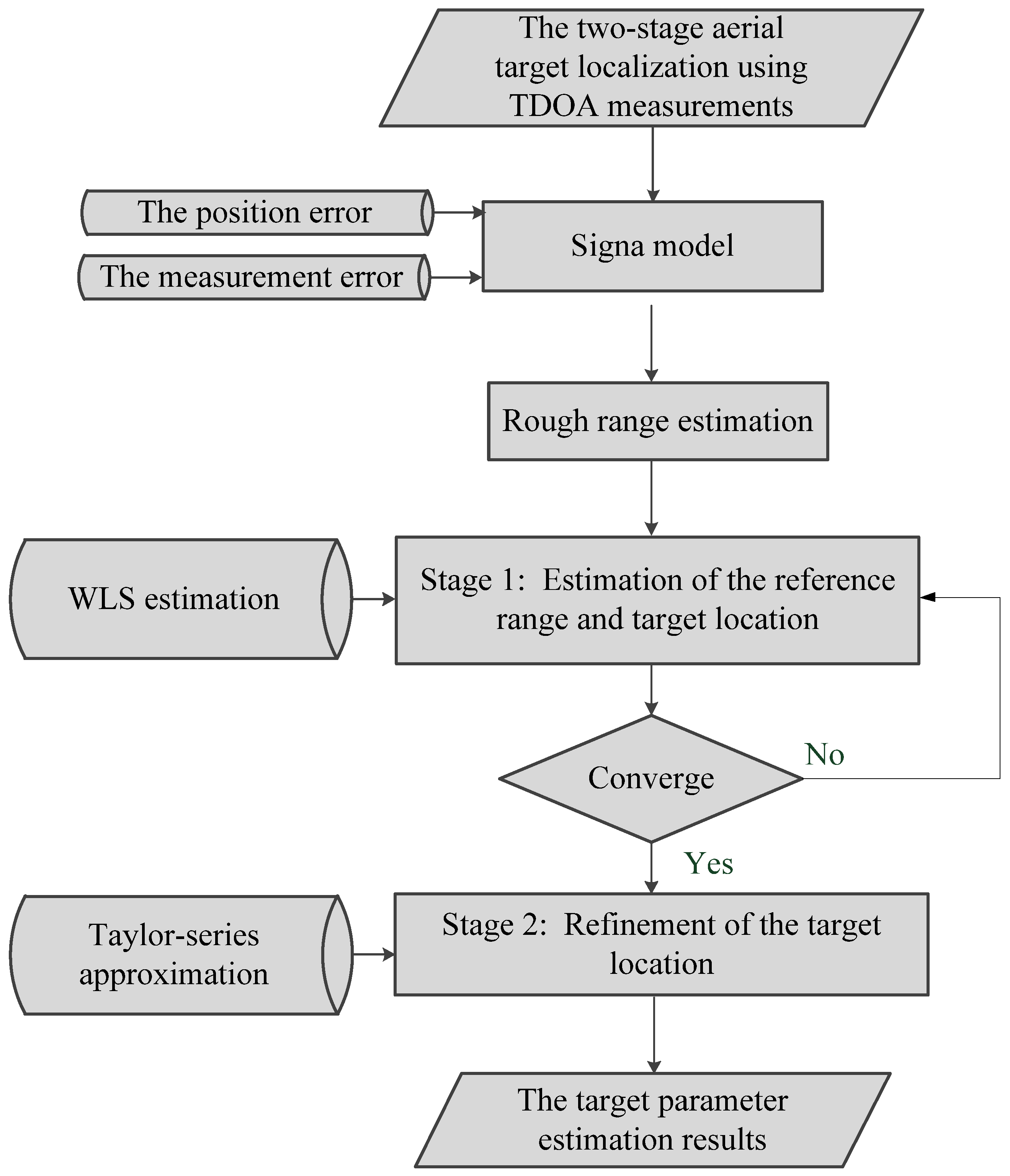
2. Materials and Methods

2.1. Basic Signal Model

Consider a space–air integrated distributed radar system composed of a geostationary Earth orbit (GEO) spaceborne radar, served as a transmitter and K unmanned aerial vehicle (UAV) airborne radars as receivers, as shown in Figure 1. When the measurement error and the satellite orbit error are considered, we can obtain the GEO satellite navigation position s ¯ = [ s ¯ x , s ¯ y , s ¯ z ] T by invoking the imprecise information from the Global Navigation Satellite System (GNSS). However, the actual position s = [ s x , s y , s z ] T is unknown and is expressed by s = s ¯ + Δ s , where Δ s = [ Δ s x , Δ s y , Δ s z ] T represents the three-dimensional (3D) GEO satellite position error. Without loss of generality, Δ s obeys Gaussian distribution with zero mean and the following covariance matrix:
Q s = E Δ s Δ s T .
Likewise, the actual position of the k-th UAV position u k = [ u x k , u y k , u z k ] T is perturbed from the navigation position u ¯ k = [ u ¯ x k , u ¯ y k , u ¯ z k ] T by its 3D platform position error Δ u k = [ Δ u x k , Δ u y k , Δ u z k ] T due to the measurement uncertainty and nonstationary flight motion. Here, position errors among different UAVs are assumed uncorrelated with each other, and the k-th UAV position error is Gaussian distributed with zero mean and the following covariance matrix:
Q u = E Δ u Δ u T ,
where Δ u = [ Δ u 1 T , Δ u 2 T , , Δ u K T ] T .
To cater to a more practical localization scenario, the range measurements from the GEO satellite to an aerial target of interest, to UAVs are gathered to perform the target localization, with the assistance of the prior statistics of position errors, in our designed framework. In view of the relationship between the TDOA and the range difference of arrival (RDOA), τ = r / c , where c is the speed of light. It is worthwhile to note that we interchange the terms TDOA and RDOA hereafter for their equivalence. The aerial target to be located is at the coordinate p = [ x p , y p , z p ] T ; then, the bistatic range between the navigation position from the GEO satellite and the k-th UAV navigation position is expressed as
r T k o = r T o + r k o = s ¯ p 2 + u ¯ k p 2 .
Furthermore, the corresponding bistatic pseudo-range for the transmit/receive pair ( T , k ) , where T denotes the transmitter, is given by
r T k = r ¯ T + r k ,
where r ¯ T = | | s p | | 2 represents the noiseless range from the GEO satellite to the target, and r k = r ¯ k + n k indicates the noisy range measurement from the target to the k-th receiving radar; r ¯ k = | | u k p | | 2 is the noiseless range, and n k is the measurement noise. By differencing the range measurement r T k to the reference one, i.e., r T 1 , we can obtain the k-th TDOA measurement as follows:
r k 1 = r T k r T 1 = u k p 2 u 1 p 2 + n k 1 ,
where n k 1 = n k n 1 is the TDOA noise measurement. Collecting the TDOA measurements from all receiving radars into a vector, Equation (5) can be written as
r 1 = r 21 , , r K 1 T = r ¯ 1 + n 1 ,
where r ¯ 1 = [ r ¯ 21 , , r ¯ K 1 ] T represents the TDOA measurement vector for the navigation position with r ¯ k 1 = | | u k p | | 2 | | u 1 p | | 2 , and n 1 = [ n 21 , , n K 1 ] T represents the TDOA noise measurement vector obeying the zero-mean Gaussian distribution with the following covariance matrix:
Q n 1 = E n 1 n 1 T .
The TDOA noise measurement vector n 1 and the position error vector Δ u are mutually uncorrelated.
The objective of this paper is to perform 3D target localization with the number of receiving radars as low as possible in the presence of the GEO satellite and UAV position uncertainties. In the next section, we propose a two-stage WLS solution to tackle this problem. It should be emphasized that our localization method is not difficult to extend to the case of multiple transmitters, without needing many modifications.

2.2. Stage 1: Estimation of the Reference Range and the Target Location in an Iterative Way

The noiseless TDOA measurement r ¯ k 1 = r ¯ T k r ¯ T 1 and the bistatic range r ¯ T k = r ¯ T + r ¯ k can be combined, yielding
r ¯ k 1 = r ¯ k r ¯ 1 .
From Equation (8), we show that the influence of the GEO satellite position error on target localization can be removed by employing TDOAs. Rearranging Equation (8) as r ¯ k 1 + r ¯ 1 = r ¯ k and squaring both sides, we can get the following [21]:
r ¯ k 1 2 + 2 r ¯ k 1 r ¯ 1 = S k S 1 2 u k u 1 T p ,
where S k = u k T u k . Moreover, substituting u k = u ¯ k + Δ u k and r ¯ k 1 = r k 1 n k 1 into Equation (9) and ignoring the second-order error terms [22,23], the equation error of Equation (9) is approximately expressed as
ς k 1 2 n k 1 r 1 o 2 u ¯ k p T Δ u k + 2 u ¯ 1 p T Δ u 1 r k 1 2 S ¯ k + S ¯ 1 + 2 u ¯ k u ¯ 1 T p + 2 r k 1 r 1 o ,
where S ¯ k = u ¯ k T u ¯ k . Stacking Equation (10) for all transmit/receiver pairs in a matrix form yields
ς 1 = h 1 G 1 φ 1 ,
where φ 1 = [ p T , r 1 o ] T , ς 1 = [ ς 21 , , ς K 1 ] T , and
h 1 = r 21 2 S ¯ 2 + S ¯ 1 r K 1 2 S ¯ K + S ¯ 1 ,
G 1 = 2 u ¯ 2 u ¯ 1 T r 21 u ¯ K u ¯ 1 T r K 1 .
Note that the number of unknown parameters in φ 1 is four, while the obtained TDOA measurement number is ( K 1 ) . As a result, if we apply the canonical Chan-Ho technique to solve the problem directly, then K 5 receiving radars are deployed to meet the requirement of the parameter identifiability. Otherwise, the larger number of unknown parameters than TDOA measurements would induce a trivial localization result. Hence, we rewrite Equation (11) as
ς 1 = h 1 + 2 r 1 r 1 o G 1 p ,
where
G 1 = 2 u ¯ 2 u ¯ 1 T u ¯ K u ¯ 1 T .
Invoking the Gauss–Markov theorem [38] in Equation (14), we can obtain the WLS estimate of p by minimizing ς 1 T W 1 ς 1 as
p ^ = ( G 1 T W 1 G 1 ) 1 G 1 T W 1 h 1 + 2 r 1 r 1 o ,
where W 1 = E { ς 1 ς 1 T } 1 is the weighting matrix. Similar to the techniques in [21,26], we substitute p ^ in Equation (16) back into the reference range r 1 o , yielding
( G 1 T W 1 G 1 ) 1 G 1 T W 1 h 1 + 2 r 1 r 1 o u ¯ 1 2 r 1 o .
After some mathematical manipulations, we obtain
A r 1 o 2 + B r 1 o + C = 0 ,
where
A = 4 ( G 1 T W 1 G 1 ) 1 G 1 T W 1 r 1 2 2 1 ,
B = 4 ( G 1 T W 1 G 1 ) 1 G 1 T W 1 h 1 u ¯ 1 T ( G 1 T W 1 G 1 ) 1 G 1 T W 1 r 1 ,
C = ( G 1 T W 1 G 1 ) 1 G 1 T W 1 h 1 u ¯ 1 2 .
The weighted matrix W 1 can be derived as a function of the statistics of position error in the a priori information. From Equation (10), rearranging ς 1 yields
ς 1 = A 1 n 1 + B 1 Δ u = A 1 B 1 n 1 Δ u ,
where
A 1 = 2 r 2 o 0 0 r K o ,
B 1 = 2 u ¯ 1 p T u ¯ k p T 0 1 × 3 u ¯ 1 p T u ¯ 1 p T 0 1 × 3 u ¯ k p T ,
In this way, the weighted matrix W 1 is
W 1 = A 1 Q n 1 A 1 T + B 1 Q u B 1 T 1 .
Nevertheless, the nominal ranges and directions from the target to the receiving radars in A 1 and B 1 are unknown for the WLS solution in Equation (16). Here, we would introduce an iterative way to update W 1 and p ^ alternatively. For the first iteration, we assume that the target ranges and directions are approximately equal; then, A 1 and B 1 can be simplified to
A 1 I K 1 ,
B 1 1 1 × 3 1 1 × 3 0 1 × 3 1 1 × 3 1 1 × 3 0 1 × 3 1 1 × 3 .
Solving the quadratic Equation (18) to produce the estimate of reference range r ^ 1 o and substituting it back into Equation (16), we obtain the first-stage target localization estimate:
p ^ I = ( G 1 T W 1 G 1 ) 1 G 1 T W 1 h 1 + 2 r 1 r ^ 1 o .
Most importantly, we emphasize here that there must be only four radars participating in the first stage even though excess radars are available.

2.3. Stage 2: Refinement of the Target Location Using Taylor Series Approximations

Since the aerial target localization is implemented by a lower number of receiving radars, the target localization accuracy can be further improved by applying the first-order Taylor series expansion [24,25,39] to r k 1 at the first-stage estimate of the target location, i.e.,
r k 1 u ¯ k p ^ I 2 u ¯ 1 p ^ I 2 + α k α 1 T Δ p I + α k T Δ u k α 1 T Δ u 1 + n k 1 ,
where Δ p I = p p ^ I is the estimation bias of the target location in the first stage, and α k = ( u ¯ k p ^ I ) / | | u ¯ k p ^ I | | 2 is the unit steering vector from the target to the k-th receiving radar. Similar to Equation (10), the equation error of Equation (29) is
ς k 2 = n k 1 + α k T Δ u k α 1 T Δ u 1 = r k 1 u ¯ k p ^ I 2 + u ¯ 1 p ^ I 2 α k α 1 T Δ p I .
Once again, stacking Equation (30) leads to
ς 2 = h 2 G 2 Δ p ,
where ς 1 = [ ς 21 , , ς K 1 ] T ,
h 2 = r 21 u ¯ 2 p ^ I 2 + u ¯ 1 p ^ I 2 r K 1 u ¯ K p ^ I 2 + u ¯ 1 p ^ I 2 ,
G 2 = α 2 α 1 T α K α 1 T .
Then, the WLS solution of Δ p I remaining in the first stage is
Δ p ^ I = G 2 T W 2 G 2 1 G 2 T W 2 h 2 ,
where W 2 = E { ς 2 ς 2 T } 1 . Now, let us calculate the weighted matrix W 2 . By rearranging ς 2 , we get
ς 2 = A 2 n 1 + B 2 Δ u = A 2 B 2 n 1 Δ u .
Similarly, the iteration technique is used again, and the initial guesses of A 2 and B 2 are given by
A 2 = A 1 ,
B 2 = α 1 T α 2 T 0 1 × 3 α 1 T α 1 T 0 1 × 3 α K T .
Hence, the weighted matrix W 2 is
W 2 = A 2 Q n 1 A 2 T + B 2 Q u B 2 T 1 .
Lastly, we combine Equations (28) and (34), and the second-stage target localization becomes
p ^ II = p ^ I + Δ p ^ I .
Furthermore, the flowchart of the proposed TDOA-based target localization method is shown in Figure 2.

2.4. Cramer–Rao Lower Bound (CRLB)

The CRLB is commonly used as a benchmark to place a lower bound of any unbiased estimator for the parameter of interest [38]. In this section, the CRLB for target localization is derived in order to evaluate the performances of different methods.
The parameter vector of interest is defined as follows:
θ p T , u T T ,
which is collected from the actual position of receiving radars. The logarithmic version of the probability density function (PDF) is constructed by utilizing TDOA measurements and a priori statistics of position errors:
u = u 1 T , u 2 T , , u K T T ,
ln f θ = 1 2 r 1 r ¯ 1 H Q n 1 1 r 1 r ¯ 1 1 2 u u ¯ H Q u 1 u u ¯ ,
where all UAV navigation positions are arranged into a vector as follows:
u ¯ = [ u ¯ 1 T , u ¯ 2 T , , u ¯ K T ] T .
Then, the CRLB of parameter vector θ , calculated by the inversion of the Fisher information matrix (FIM), is given by
C R L B θ = J 1 θ = E 2 ln f θ θ θ T 1 = X Y Y T Z 1 ,
where
X = E 2 ln f θ p p T 1 = r ¯ 1 p T Q n 1 1 r ¯ 1 p ,
Y = E 2 ln f θ p u T 1 = r ¯ 1 p T Q n 1 1 r ¯ 1 u ,
and
Z = E 2 ln f θ u u T 1 = r ¯ 1 u T Q n 1 1 r ¯ 1 u + Q u 1 ,
with the Jacobian transformation matrices
r ¯ 1 p = u ¯ 2 p | | u 2 p | | 2 u ¯ 1 p | | u 1 p | | 2 , , u ¯ K p | | u K p | | 2 u ¯ 1 p | | u 1 p | | 2 ,
and
r ¯ 1 u = u ¯ 1 p | | u 1 p | | 2 u ¯ 1 p | | u 1 p | | 2 u ¯ 2 p | | u 2 p | | 2 0 0 u ¯ K p | | u K p | | 2 .
Furthermore, we apply the matrix inverse lemma [40] to Equation (44). The CRLB for target localization is modified as follows [16]:
C R L B p = X 1 + X 1 Y Z Y T X 1 Y 1 Y T X 1 .
Lastly, the minimum variance of the target location error is calculated by the matrix trace in Equation (50).

3. Results

This section provides two cases of experiments, where the minimum number of receiving radars for TDOA aerial target localization, i.e., K = 4 is evaluated first, followed by the results for the cases of more receiving radars. The WLS-Ho method [22,23] and the WLS-Mao method [25] are introduced as the compared methods. It is assumed that the radar transmitter is equipped on a GEO satellite, with an altitude of 36,000 km. Unless otherwise specified, the signal carrier frequency is 1.25 GHz. The unequal target SNRs are measured with respect to different bistatic ranges. Here, the 3D position errors of the satellite transmitter and receiving radars are both Gaussian-distributed. For each dimension, both types of position errors are zero mean, while their variances are fixed as 100 m and 0.25 m, respectively. All results are averaged over 2000 independent Monte Carlo trials.

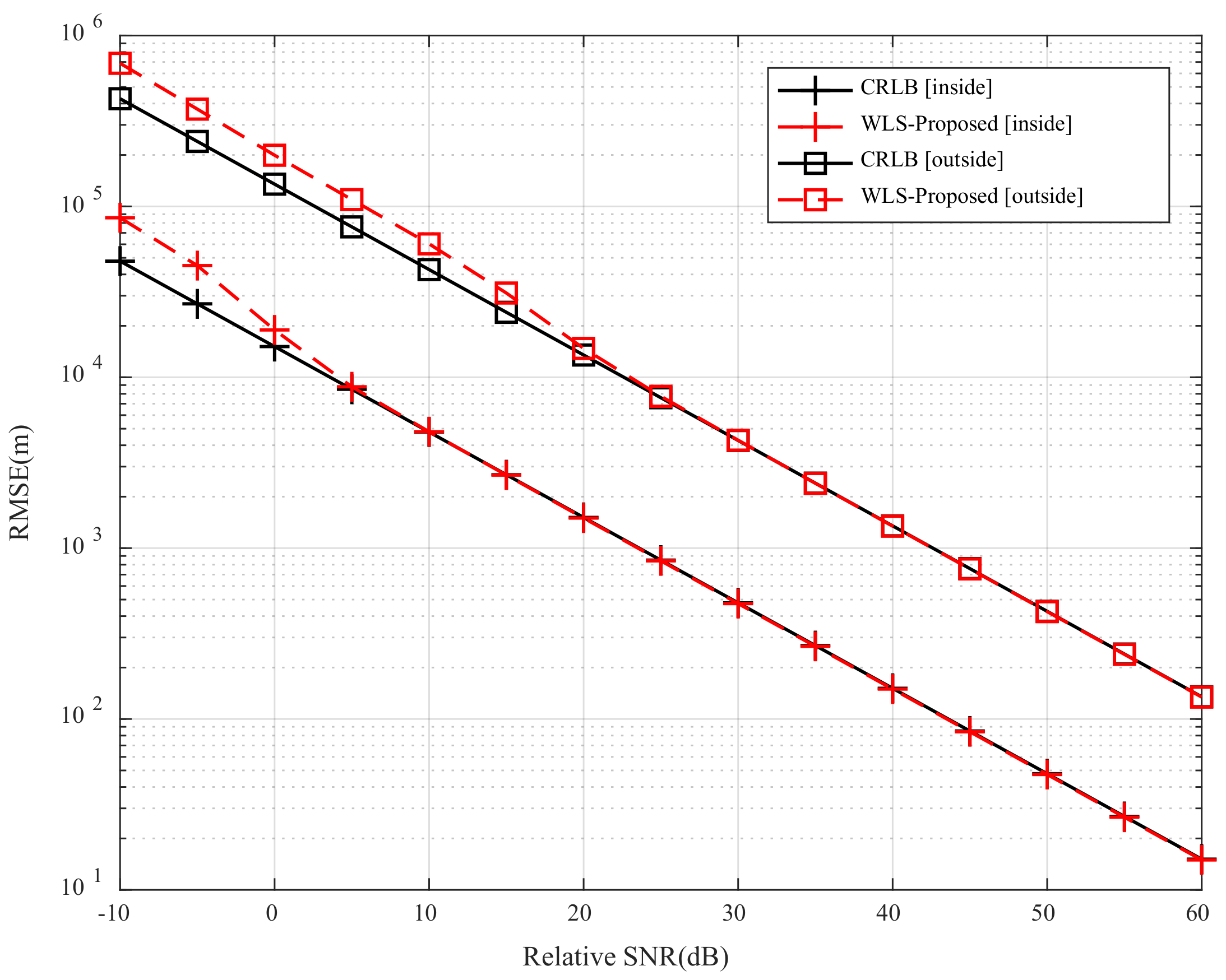
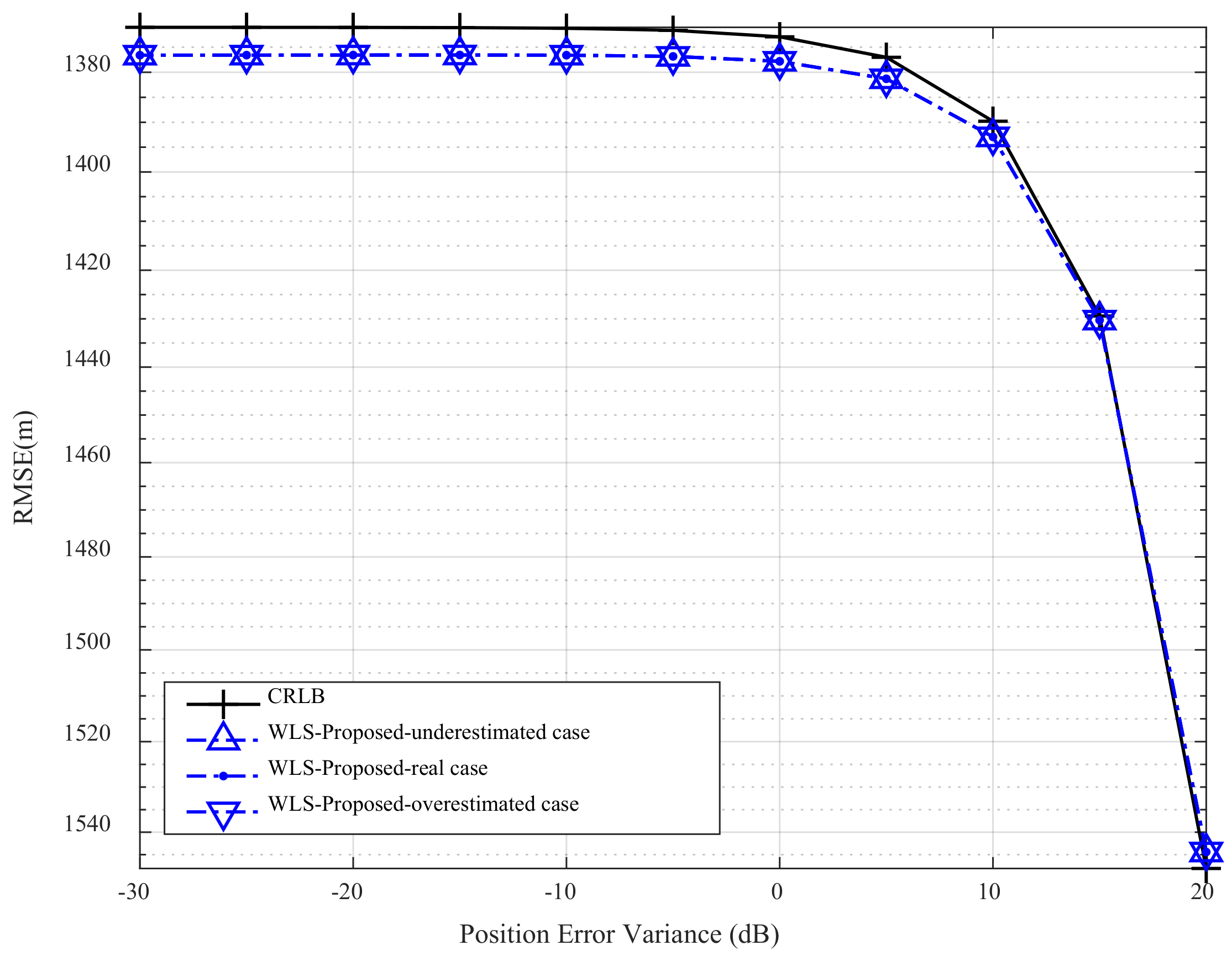
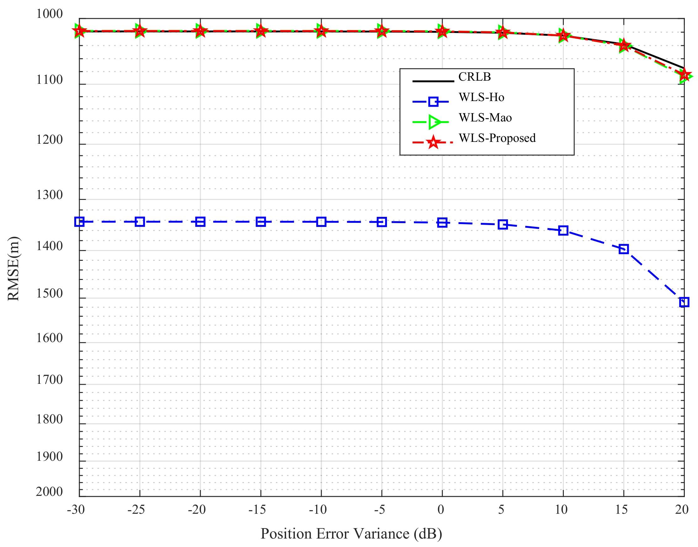
3.1. TDOA Target Localization with the Minimum Number of Radars

First, we consider the target localization in the absence of position errors. The UAV navigation positions are at the coordinates [100 × 103, 100 × 103, 23 × 103]T m, [200 × 103, 300 × 103, 22 × 103]T m, [−400 × 103, 100 × 103, 23 × 103]T m, and [200 × 103, 300 × 103, 25 × 103]T m, respectively. Under the minimum number of four receiving radars, the RMSEs of the target location versus the relative SNR are depicted in Figure 3. The relative SNR is defined as the SNR calculated relative to the reference receiving radar. The RMSE is computed as R M S E = u = 1 U p u p 2 2 / U , where p u is the u-th target location estimation, and U is the trail number. The black solid lines denote the CRLB, and the red dashed lines represent the proposed method, where the cases of the target inside and outside the radar network are marked by the plus sign and square, respectively. In Figure 3, we show that, as the relative SNR increases, the RMSE of the target location is decreased, or the localization accuracy is improved. In high-SNR regions, the proposed method can approach the theoretical CRLB. Compared to other WLS methods, the proposed method additionally considers the relationship between the target location and the reference range. Hence, by substituting the location parameters into the reference range, the estimation progresses of the target location and the reference range can be separated, which yields a lower required number of radars for the localization. After the target location is estimated in Stage 1, we can further refine the estimation results using the Taylor series approximation method in Stage 2, regardless of whether the position of the reference radar is uncertain or not. In this way, the influence of the position uncertainty weakens. Meanwhile, it is not difficult to demonstrate that a more distributed radar configuration yields better localization accuracy. Owing to the parameter unidentifiability of either the WLS-Ho method or the WLS-Mao method under four radars, their results are trivial and are not displayed here.
Then, we consider the case of the radar network with position errors. Still under four radars, Figure 4 exhibits the RMSE of the localization versus the relative SNR. We employ the plus sign and circle to represent the localization in the absence and in the presence of the position errors, respectively. Again, in both cases, our proposed method could attain the CRLB criteria as the relative SNR increases, implying that this method is robust enough against the position uncertainty. Moreover, we show that the localization performance of the former case in high-SNR regions deviates from that of the latter case, which is explained by the result of limited position accuracy. Once the position accuracy is improved, one can expect a more relatively accurate localization.
Next, we study the case of the RMSE of the localization versus UAV position error variance in Figure 5. The upward-pointing triangle, point, and downward-pointing triangle represent the cases with error variance underestimation, exactly known, and overestimation, where the three cases correspond to 10% of the error variance, unchanged error variance, and tenfold the real error variance, respectively. As the position error variance increases, we can show that the localization accuracies gradually shrink. Nevertheless, we find that the proposed method can still approximate the performance bound to a certain extent. In Figure 5, the RMSEs of these three cases perform nearly the same localization; thus, we conclude that the erroneous error variance may not play a major role in localization performance, which paves a way for the practical engineering applications.
Furthermore, to evaluate the localization accuracy for a given location of the target under a specified radar network, the GDOP metric [14,39] is invoked to address this issue. The GDOP metric is especially applied in the GPS system which is used to measure how the localization accuracy of an object in a fixed position can be attained. The GDOP is defined as
G D O P = 1 c σ x 2 + σ y 2 + σ z 2 σ ε 2 ,
where σ x 2 , σ y 2 , and σ z 2 are the x-, y-, and z-dimensional estimation variances, respectively, and σ ε 2 is the TDOA noise measurement variance. From Equation (51), it is easy to conclude that the GDOP is purely a geometric localization evaluation tool, where the SNR factor is precluded. Under our case of the minimum number of receiving radars, the CRLB-GDOP result and WLS-proposed-GDOP result are shown in Figure 6, where the red pentagrams are the positions of the receiving radars, and the contours represent the localization accuracy that a given target can obtain. A relative SNR of 20 dB is assumed in the simulation. From Figure 6, we can see that, if the aerial target is located inside the virtual polygon by the receiving radars in a relative way, then the proposed method enables a satisfied TDOA localization accuracy. On the contrary, if the object is outside that polygon, the estimation result is badly deteriorated, especially along the line formed by any two radars. To explain this, we notice that the observation angles between the target and the radars are quite different for the former case, whereas the angles among them appear somewhat approximately equal for the latter. With more spatial diversity of the system, the method can attain better localization accuracy. These different observation angles are the foundation for the localization.

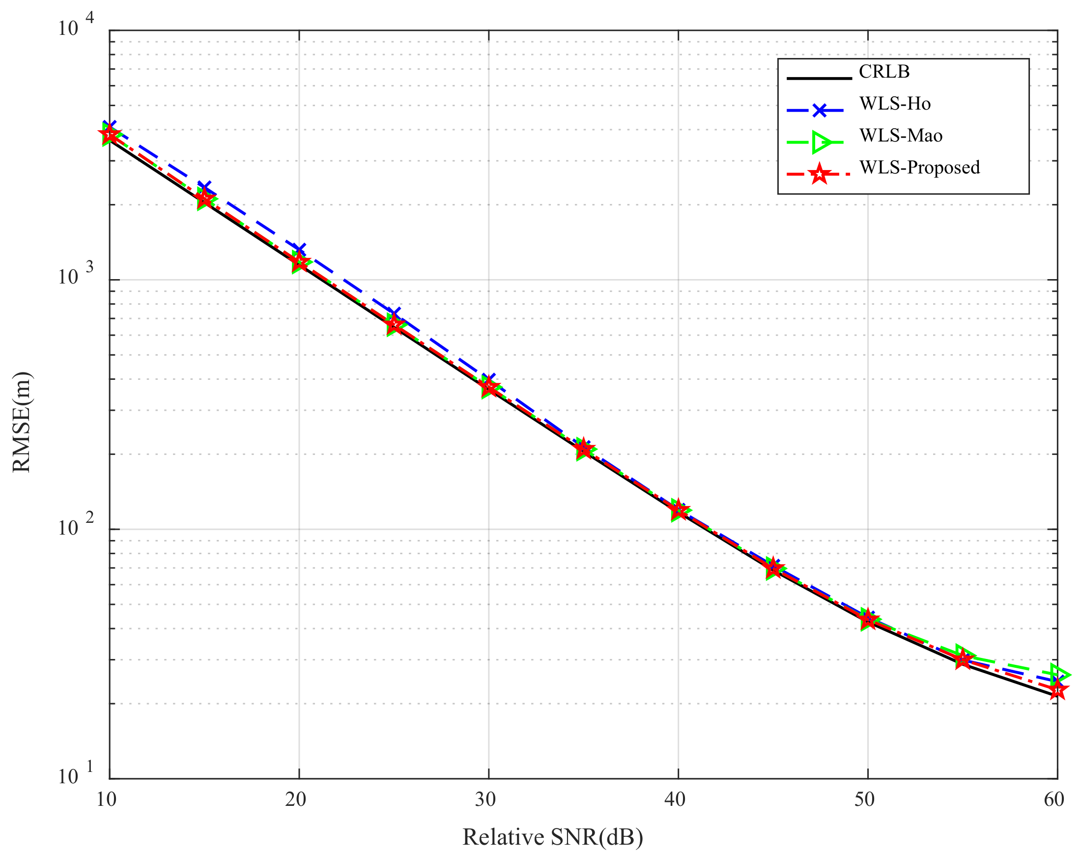
3.2. TDOA Target Localization with more Receiving Radars

Next, we consider the number of five receiving radars. The UAVs’ nominal positions are unchanged except that a new one is added at the coordinates [0 × 103, 500 × 103, 25 × 103] T m. The RMSE of the target location versus the relative SNR is demonstrated in Figure 7. The CRLB, WLS-Ho method, WLS-Mao method, and our WLS-proposed method are represented by the black line, blue dashed line marked with a cross, green dashed line marked with a right-pointing triangle, and red dash-dotted line marked with a pentagram, respectively. We observe that the estimation accuracy of the WLS-proposed method is slightly better than that of the WLS-Ho method and WLS-Mao method. Resulting from the approximate error shown in Equation (17), the localization accuracy may be disappointing with low SNRs. Nevertheless, from the view of practical engineering, the SNRs of receiving radars would be designed to exceed 13 dB in most cases. Thus, we can conclude that the influence of this approximation is very slight.
In Figure 8, we show that, as the position error variance increases, the RMSEs of the target location are larger. For the WLS-Ho method, the reference range is the nonlinear function of the target location; hence, the deviations occur as the variance increases. The localization accuracies of the WLS-Mao method and WLS-proposed method could nearly attain that of the CRLB, whereas our method performed slightly better.
Lastly, we present the CRLB-GDOP, WLS-Ho-GDOP, WLS-Mao-GDOP, and WLS- proposed-GDOP results to close the discussion. As shown in Figure 9, the proposed method achieves better localization accuracy compared to other state-of-the-art methods. Again, more angle divergence means better localization accuracy. As for the influence of the receiving radar selection for optimal aerial target localization, it deserves further investigation.

4. Discussions

In this paper, a two-stage target localization method using TDOA measurements was developed with a minimum number of radars. Under position uncertainties, the novel TDOA-based localization method is capable of locating targets under only four radars with comparative localization accuracy in comparison to the CRLB. The localization process can be mainly divided into two stages: (1) the 3D WLS target estimates are substituted into the reference range equation to obtain a quadratic function of the reference range, and then the reference range and the target coordinates are updated in an iterative manner; (2) the target coordinates are further refined by applying the· first-order Taylor series expansion at the estimated target location in the first stage.
It should be emphasized that only four radars must be used to localize the target in the first stage even though the total radar number exceeds that number. Otherwise, the target localization would badly deteriorate. All radars involved can be considered in the second stage to improve the localization.
Compared to the WLS-Ho method, our proposal does not introduce the nonlinear approximate error between the reference range and the target location, thus alleviating the sensitivity to position errors. In contrast to the WLS-Mao method, we have more accurate target estimates in the first stage, which is vital for the second-stage refinement.
In the case of multiple transmitting radars, the proposed method can also be applied after slight modifications by taking both the measurement errors and position errors into consideration.

5. Conclusions

For most cases of two-stage target TDOA localization methods, there are five or more receiving radars to support the necessary parameter identifiability. However, the additional deployment of radars is extremely expensive or impossible in some practical scenarios. Hence, in this paper, we propose a novel two-stage WLS target localization method to alleviate exceptional employment. We first formulate the iteration between the target location and the reference range, and then the Taylor series approximation is made to refine the target location. Simulation results show that the proposed method outperformed the existing WLS techniques under four radars and was competitive with them when using more radars. The proposed method is also applicable to localization using near-space platforms and ground-based platforms. Our future work will concentrate on localization involving clock synchronization errors and phase errors to generalize our development.

Author Contributions

Conceptualization, J.C. and Y.L.; methodology, J.C. and Y.L.; software, J.C.; validation, X.Y. and F.L.; formal analysis, C.D.; investigation, C.L. and C.D.; resources, C.D. and Y.L.; data curation, C.D. and Y.L.; writing—original draft preparation, J.C.; writing—review and editing, J.C., W.W. and Y.L.; visualization, J.C. and Q.L.; supervision, X.Y.; project administration, C.L.; funding acquisition, Y.L. All authors have read and agreed to the published version of the manuscript.

Funding

This research was funded by the National Natural Science Foundation of China under grant number 62107033, the National Defense Science and Technology Foundation Strengthening Plan Fund under grant number 2022-JCJQ-JJ-0202, the Sustainedly Supported Foundation by the National Key Laboratory of Science and Technology on Space Microwave under grant number HTKJ2022KL504004, the CAST Foundation of the Fifth Academy under grant number Y22-CASTJJ-02, and the Outstanding Youth Foundation of the Fifth Academy, Aerospace Science, and Technology Group under Grant Y22-RCWYJQ1-01.

Acknowledgments

The authors are grateful to the University of Electronic Science and Technology of China for supporting this research. The authors also thank the associate editor and anonymous reviewers for their insightful comments and suggestions.

Conflicts of Interest

The authors declare no conflict of interest.

References

  1. Richard, A.P. Information Warfare and Electronic Warfare Systems, 1st ed.; Artech House: Norwood, MA, USA, 2013. [Google Scholar]
  2. Reza, A.; Buehrer, R.M. Handbook of Position Location: Theory, Practice and Advances, 1st ed.; Wiley-IEEE Press: Hoboken, NJ, USA, 2019. [Google Scholar]
  3. Malanowski, M. Signal Processing for Passive Bistatic Radar, 1st ed.; Artech House: Norwood, MA, USA, 2019. [Google Scholar]
  4. Weiss, A.J. Direct position determination of narrow band radio frequency transmitters. IEEE Signal Process. Lett. 2004, 11, 513–516. [Google Scholar] [CrossRef]
  5. Bar-Shalom, O.; Weiss, A.J. Direct positioning of stationary targets using MIMO radar. Signal Process. 2011, 91, 2345–2358. [Google Scholar] [CrossRef]
  6. Tzore, E.; Weiss, A.J. Expectation-maximization algorithm for direct position determination. Signal Process. 2017, 133, 32–39. [Google Scholar] [CrossRef]
  7. Smith, J.O.; Abel, J.S. Closed-form least-squares source location estimation from range difference measurements. IEEE Trans. Acoust. Speech Signal Process. 1987, 35, 1661–1669. [Google Scholar] [CrossRef]
  8. Hyuksso, S.; Wonzoo, C. Target localization using double-sided range measurements in distributed MMO systems. Sensors 2019, 19, 2524. [Google Scholar]
  9. Zhang, Y.; Ho, K.C. Multistatic localization in the absence of transmitter position. IEEE Trans. Signal Process. 2019, 67, 4745–4760. [Google Scholar] [CrossRef]
  10. Mellen, G., II; Pachter, M.; Raquet, J. Closed-form solution for determining emitter location using time difference of arrival measurements. IEEE Trans. Aerosp. Electron. Syst. 2003, 39, 1056–1058. [Google Scholar] [CrossRef]
  11. Bhatta, B. Global Navigation Satellite Systems: New Technologies and Applications, 2nd ed.; CRC Press: Boca Raton, FL, USA, 2021. [Google Scholar]
  12. Xie, G. Principles of GPS, GLONASS, and Galileo, 1st ed.; Publishing Housing of Electronics Industry: Beijing, China, 2015. [Google Scholar]
  13. Kenneth, W.; So, H.C. A study of two-dimensional sensor placement using time difference-of-arrival-measurements. Digit. Signal Process. 2009, 19, 650–659. [Google Scholar]
  14. Nguyen, N.H.; Dogancay, K. Optimal geometry analysis for multistatic TOA localization. IEEE Trans. Signal Process. 2016, 64, 4180–4193. [Google Scholar] [CrossRef]
  15. Sadeghi, M.; Behnia, F.; Amiri, R. Optimal sensor placement for 2-D range-only target localization in constrained sensor geometry. IEEE Trans. Signal Process. 2020, 68, 2316–2327. [Google Scholar] [CrossRef]
  16. Fang, B.T. Simple solutions for hyperbolic and related position fixes. IEEE Trans. Aerosp. Electron. Syst. 1990, 26, 748–753. [Google Scholar] [CrossRef]
  17. Friedlander, B. A passive localization algorithm and its accuracy analysis. IEEE J. Ocean. Eng. 1987, 12, 234–245. [Google Scholar] [CrossRef]
  18. Schay, H.C.; Robinson, A.Z. Passive source localization employing intersecting spherical surfaces from time-of-arrival differences. IEEE Trans. Acoust. Speech Signal Process. 1987, 35, 1223–1225. [Google Scholar] [CrossRef]
  19. Foy, W.H. Position-location solutions by-Taylor-series estimation. IEEE Trans. Aerosp. Electron. Syst. 1976, 12, 187–194. [Google Scholar] [CrossRef]
  20. Koyaisaruch, L.; Ho, K.C.; So, H.C. Modified Taylor-series method for source and receiver localization using TDOA measurements with erroneous receiver positions. In Proceedings of the 2005 IEEE International Symposium on Circuits and Systems (ISCAS), Kobe, Japan, 23–26 May 2005; IEEE: Piscataway, NJ, USA, 2005. [Google Scholar]
  21. Chan, Y.T.; Ho, K.C. A simple and efficient estimator for hyperbolic location. IEEE Trans. Signal Process. 1994, 42, 1905–1915. [Google Scholar] [CrossRef]
  22. Ho, K.C.; Kovavisaruch, L.; Parikh, H. Source localization using TDOA with erroneous receiver positions. In Proceedings of the 2004 IEEE International Symposium on Circuits and Systems (ISCAS), Vancouver, BC, Canada, 23–26 May 2004; IEEE: Piscataway, NJ, USA, 2004. [Google Scholar]
  23. Ho, K.C.; Lu, X.N. Source localization using TDOA and FDOA measurements in the presence of receiver location errors: Analysis and solution. IEEE Trans. Signal Process. 2007, 55, 684–696. [Google Scholar] [CrossRef]
  24. Zhang, F.R.; Sun, Y.M.; Zou, J.F.; Zhang, D.; Wan, Q. Closed-form localization method for moving target in passive multistatic radar network. IEEE Sens. J. 2020, 20, 980–990. [Google Scholar] [CrossRef]
  25. Mao, Z.; Su, H.T.; He, B.; Jing, X. Moving source localization in passive sensor network with location uncertainty. IEEE Signal Process. Lett. 2021, 28, 823–827. [Google Scholar] [CrossRef]
  26. Ma, H.; Antoniou, M.; Stove, A.G.; Winkel, J.; Cherniakov, M. Maritime moving target localization using passive GNSS-based multistatic radar. IEEE Trans. Geosci. Remote Sens. 2018, 56, 4808–4819. [Google Scholar] [CrossRef]
  27. Yang, L.; Ho, K.C. An approximately efficient TDOA localization algorithm in closed-form for locating multiple disjoint sources with erroneous sensor positions. IEEE Trans. Signal Process. 2009, 57, 4598–4615. [Google Scholar] [CrossRef]
  28. Sun, M.; Ho, K.C. An asymptotically efficient estimator for TDOA and FDOA positioning of multiple disjoint-sources in the presence of sensor location uncertainties. IEEE Trans. Signal Process. 2011, 59, 3434–3440. [Google Scholar]
  29. Liu, Y.; Guo, F.C.; Yang, L.; Jiang, W. An improved algebraic solution for TDOA localization with sensor position errors. IEEE Commun. Lett. 2015, 19, 2218–2221. [Google Scholar] [CrossRef]
  30. Cheung, K.W.; Ma, W.K.; So, H.C. Accurate approximation algorithm for TOA-based maximum likelihood mobile location using semidefinite programming. In Proceedings of the 2004 IEEE International Conference on Acoustics, Speech and Signal Processing (ICASSP), Montreal, QC, Canada, 17–21 May 2004; IEEE: Piscataway, NJ, USA, 2004. [Google Scholar]
  31. Yang, K.; Wang, G.; Luo, Z.Q. Efficient convex relaxation methods for robust target localization by a sensor network using time differences of arrivals. IEEE Trans. Signal Process. 2009, 57, 2775–2784. [Google Scholar] [CrossRef]
  32. Zhao, R.C.; Wang, G.; Ho, K.C. Accurate semidefinite relaxation method for elliptic localization with unknown transmitter position. IEEE Trans. Wirel. Commun. 2021, 20, 2746–2760. [Google Scholar]
  33. Amiri, R.; Behnia, F.; Zamani, F. Asymptotically efficient target localization from bistatic range measurements in distributed MIMO radars. IEEE Signal Process. Lett. 2017, 20, 299–303. [Google Scholar] [CrossRef]
  34. Amiri, R.; Behnia, F.; Mohammad, A.M.S. Efficient positioning in MMO radars with widely separated antennas. IEEE Commun. Lett. 2017, 21, 1569–1572. [Google Scholar] [CrossRef]
  35. Amiri, R.; Behnia, F.; Sadr, M. Exact solution for elliptic localization in distributed MIMO radar systems. IEEE Trans. Veh. Technol. 2018, 67, 1075–1086. [Google Scholar] [CrossRef]
  36. Amiri, R.; Behnia, F.; Noroozi, A. Efficient joint moving target and antenna localization in distributed MIMO radars. IEEE Trans. Wirel. Commun. 2019, 18, 4425–4435. [Google Scholar] [CrossRef]
  37. Amiri, R.; Kazemi, R.; Behnia, F.; Noroozi, A. Efficient elliptic localization in the presence of antenna position uncertainties and clock parameter imperfections. IEEE Trans. Veh. Technol. 2019, 68, 9797–9805. [Google Scholar] [CrossRef]
  38. Kay, S.M. Fundamentals of Statistical Signal Processing: Estimation Theory, 1st ed.; Prentice-Hall: Englewood Cliffs, NJ, USA, 1993. [Google Scholar]
  39. Godrich, H.; Haimovich, A.M.; Blum, R.S. Target localization accuracy gain in MIMO radar-based systems IEEE Transactions on Information Theory. IEEE Trans. Inf. Theory 2010, 56, 2783–2803. [Google Scholar] [CrossRef]
  40. Horn, R.A.; Johnson, C.R. Matrix Analysis, 2nd ed.; Cambridge University Press: Cambridge, UK, 2013. [Google Scholar]
Figure 1. The space–air integrated TDOA localization.
Remotesensing 15 02829 g001
Figure 2. The flowchart of two-stage target localization method using TDOA measurements.
Remotesensing 15 02829 g002
Figure 3. The RMSE of the target location versus relative SNR in the absence of position errors.
Remotesensing 15 02829 g003
Figure 4. The RMSE of the target location versus the relative SNR in the presence of position errors.
Remotesensing 15 02829 g004
Figure 5. The RMSE of the target location versus the UAV position error variance under different error variance estimation cases.
Remotesensing 15 02829 g005
Figure 6. GDOP results: (a) CRLB-GDOP; (b) WLS-proposed-GDOP.
Remotesensing 15 02829 g006
Figure 7. The RMSE of the target location versus the relative SNR under five radars.
Remotesensing 15 02829 g007
Figure 8. The RMSE of the target location versus the UAV position error variance under five radars.
Remotesensing 15 02829 g008
Figure 9. GDOP results: (a) CRLB-GDOP; (b) WLS-Ho-GDOP; (c) WLS-Mao-GDOP; (d) WLS-proposed-GDOP.
Remotesensing 15 02829 g009
Disclaimer/Publisher’s Note: The statements, opinions and data contained in all publications are solely those of the individual author(s) and contributor(s) and not of MDPI and/or the editor(s). MDPI and/or the editor(s) disclaim responsibility for any injury to people or property resulting from any ideas, methods, instructions or products referred to in the content.

