Modeling Phenology Combining Data Assimilation Techniques and Bioclimatic Indices in a Cabernet Sauvignon Vineyard (Vitis vinifera L.) in Central Chile

Abstract

Phenology is a science that is fundamental to crop productivity and is especially sensitive to environmental changes. In Mediterranean and semi-arid climates, vineyard phenology is directly affected by changes in temperature and rainfall distribution, being highly vulnerable to climate change. Due to the significant heterogeneity in soil, climate, and crop variables, we need fast and reliable ways to assess vineyard phenology in large areas. This research aims to evaluate the performance of the phenological data assimilation model (DA-PhenM) and compare it with phenological models based on meteorological data (W-PhenM) and models based on Sentinel-2 NDVI (RS-PhenM). Two W-PhenM approaches were evaluated, one assessing eco- and endo-dormancy, as proposed by Caffarra and Eccel (CaEc) and the widely used BRIN model, and another approach based on the accumulation of heat units proposed by Parker called the Grapevine Flowering Veraison model (GFV). The DA-PhenM evaluated corresponds to the integration between RS-PhenM and CaEc (EKF-CaEC) and between RS-PhenM and GFV (EKF-GFV). Results show that EKF-CaEc and EKF-GFV have lower root mean square error (RMSE) values than CaEc and GFV models. However, based on the number of parameters that models require, EKF-GFV performs better than EKF-CaEc because the latter has a higher Bayesian Index Criterion (BIC) than EKF-GFV. Thus, DA-PhenM improves the performance of both W-PhenM and RS-PhenM, which provides a novel contribution to the phenological modeling of Vitis vinifera L. cv Cabernet Sauvignon.

1. Introduction

Several processes of crop physiology depend on the climate at different time scales. Among them, crop phenology is fundamental as it determines crop performance over a growing season and is commonly used for agricultural planning. An accurate representation of this process is crucial for assessing crop productivity.

Global environmental changes experienced in recent decades and those predicted for the coming years affect the crop phenology, especially in areas with high climate variability, such as the Mediterranean and semi-arid zones [1,2,3,4,5]. Vineyards represent one of the most economically significant agricultural products in these areas. Thus, changes in vineyard phenology will shape management practices for strategic planning in the sector, especially regarding viticultural zoning and the selection of suitable cultivars [6,7,8,9,10].

Temperature is the main driver of grapevine (Vitis vinifera L.) phenology [11,12,13,14,15,16]. Values between 10 °C and 25 °C are optimal for vine development [17]. Temperatures between 5 and 10 °C are also critical for accumulating cold units to complete dormancy, playing a fundamental role in flowering and berry formation processes [16]. Several studies have identified that average maximum temperatures during the spring months have a strong negative correlation with the duration of the budburst–flowering interphase. In contrast, the period of the interphases (flowering–veraison and veraison–maturity) is related to the accumulation of heat forcing units. Several studies have shown a nonlinear effect of temperature on grapevine phenology, but these responses are different among cultivars [12,13,18,19,20]. In addition to temperature, soil water availability and soil physical properties impact the phenology of grapevines, with earlier flowering and veraison associated with water deficit or in dry years for rainfed vineyard systems [8,21,22].

Multiple tools have been used to represent phenology, including weather-based phenological models (W-PhenM), which are based on the accumulation of state-forcing units (SF) and the combination of chill and state-forcing units (CF) [23]. Forcing units are obtained from the difference between mean (T_m) and base temperatures (T_b), regarded as the minimum temperature required for grapevine growth. The accumulation starts on a fixed date, usually January 1st in the northern hemisphere and July 1st in the southern hemisphere, using a temperature of 10 °C [17]. In the grapevine flowering and veraison (GFV) model proposed by [24], T_b is set to 0 °C. The starting date of accumulating forcing units (t₀) corresponds to the 60th day of the year (DOY = 60) in the northern hemisphere and DOY = 242 in the southern hemisphere. CF models describe the dormancy phase [25,26], which requires accumulating chill units. When a threshold is surpassed, the accumulation of forcing units is triggered.

Grapevine phenology models with this approach are the ones proposed by [27] (CaEc) and the BRIN model [28]. The CaEc model is based on the Chuine Unified Model [25] for the accumulation of chilling during dormancy and a sigmoidal model of accumulation of forcing units for the budburst, flowering, and veraison phases. The BRIN model is an assembly between Bidabe’s Cold Action model for the dormancy phase and the Richardson model [26], based on the accumulation of growing degree hours for the budburst phase.

SF models involve estimating a few parameters; their implementation is simple and applies to wide varieties and locations. However, the predictive power of SF models is not necessarily the same for all varieties and does not properly describe the differences in development rates between stages. CF models are variety-specific and incorporate a sub-model for each phenophase, making them more complex to implement [24,27,28].

SF and CF models must be parameterized and validated site-specifically because such models do not consider the spatial variability of phenology [29,30,31,32,33,34,35]. In addition, these models depend on the availability of meteorological data that represent vineyard conditions [36,37]. Therefore, the uncertainty associated with W-PhenM lies mainly in the parameterization process, which is affected by the nature of the input data and the method used. In addition, the complexity of agricultural systems causes the parameterization, which is altered by biotic and abiotic factors and the associated agricultural management [38,39].

Phenological models based on remotely sensed data, known as land surface phenology models (LSP) [40], have the potential to overcome some of the drawbacks that SF and CF models have, especially regarding the spatial variability of phenology [41].

There are several classifications for LSP models according to (a) specific thresholds, (b) time series curvature, (c) previous or within-season phenology responses, and (d) changes in the trend of remotely sensed data [42]. The within-season approach (real-time or near real-time) aims to monitor crop development for operational planning [42,43]. The time-series curvature approach has been used in annual crops [44,45,46] and vineyards [47,48]. This method requires fitting remotely sensed data to a function to identify inflection points (dates) and local maxima and minima. Based on these methods, forest phenology has been monitored using data from moderate-resolution imaging spectroradiometry (MODIS) [49,50], which has a spatial resolution between 250 m and 1000 m and a daily temporal frequency. In crops, MODIS data have been used to analyze phenology in soybean and maize [51,52] as well as vineyards [44,53,54], and has been tested for the development of crop maps [32].

LSP is an indicator of the global dynamics of terrestrial ecosystems since it responds to environmental changes, especially temperature and precipitation. Therefore, the temporal and spatial analysis of LSP patterns provides insight into the phenology of ecosystems and the drivers involved, making it a tool that improves phenology modeling in the face of climate change scenarios [55].

Despite the potential of LSPs, the challenge of these models lies in the ability to discriminate phenological metrics when compared to field observations [45], which is due to the coarse spatial resolution of remote sensing data and the inherent complexity of the transitions between phenophases [46]. In the early stages of development, where signals can be disturbed by soil moisture conditions and the woody structure of perennial plants, it generates noise that affects data quality. Additionally, the relationship between phenology and greenness detected by remote sensing is highly dependent on the crop type, its growth dynamics, and the effects of biotic and abiotic stressors [42].

It is relevant to consider the synchronization between the greenness and the structural development of the vineyard, which is related to the coincidence between changes detected by remote sensors and those observed in the field that depends on chlorophyll concentration, soil, and leaf water content. Such synchronization is critical in the abrupt transition between dormancy and the greenness increase in bud break, poorly modeled by the curve-fitting method [56].

Another challenge for applying LSPs in Mediterranean areas, such as central Chile, corresponds to the high cloudiness usually found at the beginning of the growing season (occurring in late winter and early spring), which reduces the possibility of accessing remote sensing data. In addition, vineyards are heterogeneous surfaces that include inter-row areas, being challenging to identify the earliest phenological stages only with remote sensing data [57].

Recently, Sentinel-2, a remote sensing data source available since 2015, was used to monitor phenology in forests [58], wheat [59], rice [60], and tropical fruit trees [61]. This remote sensing data source has not been used in vineyard phenology; however, Ref. [62] evaluated the potential of Sentinel-2 to obtain information on the agronomic importance in viticulture, including the phenology.

Several authors have proposed integrating LSP data with ground-level phenological, meteorological, and soil data [42,45,57,63] as a way to overcome these difficulties.

Phenological data assimilation (DA) is the process by which remote sensing measurements or observations, transformed into phenological stages, are incorporated into W-PhenMs to calibrate, replace, or update the modeled phenological processes. DA brings the ability to reduce the difference between model-based and remote sensing estimates, provides temporal continuity to the evaluated phenomena, and updates the state variables of predictive models. However, such a framework is subject to different sources of error from remote sensing data, models, and algorithms for assimilation, optimization, and interpolation. Additionally, DA requires large amounts of data (especially remote sensing data), which implies a high computational capacity to reduce computing times [64].

The main uncertainty of DA lies in selecting the algorithm to be used for assimilation since data with different spatial (e.g., local and regional) and temporal (e.g., daily and weekly) scales are usually integrated. Furthermore, DA over large areas (regional scale) requires a previous evaluation to determine the spatial covariance of phenological patterns affected by land heterogeneity [65].

DA uses algorithms, called filters, that are applied to time series of state variables in both models (e.g., W-PhenMs) and observations (e.g., remotely sensed data) to improve the estimation of state variables [66]. The Kalman Filter (KF) and its variants have been one of the most widely used algorithms in DA [67,68,69,70].

Crop simulation models have been integrated with remote sensing data of the Leaf Area Index (LAI) and soil moisture (SM) to improve yield prediction in grain crops through KF in linear processes. For nonlinear processes, the Extended Kalman Filter (EKF), Ensemble Kalman Filter (EnKF), and Particle Filter (PF) have been adopted [71,72,73,74,75,76,77]. In vineyards, the EnKF and PF have been used to assimilate data from high-resolution thermal infrared sensors and Synthetic Aperture Radar (SAR), with the soil–vegetation–atmosphere transfer (SVAT) model to improve soil moisture modeling at the surface and root zone levels [78].

In the area of phenology, DA has made possible the evaluation of the stage of several biome types, especially those found in the Mediterranean zone [79]. Better predictions are obtained in forest ecosystems in spring (when weather is highly uncertain) [65,80]. Additionally, DA helps to identify gaps in parameter estimation and poor relationships between state variables simulated by meteorological models [81,82].

Given the potential for phenology modeling approaches described above, developing a data assimilation (DA) based model in a vineyard would improve the goodness-of-fit performance of the W-PhenM and LSP. Therefore, this research aims to evaluate a DA-based phenology model that integrates W-PhenM with the Sentinel-2 LSP in a commercial Cabernet Sauvignon vineyard in Central Chile.

2. Materials and Methods

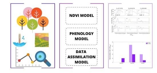
Figure 1 summarizes the data assimilation approach for phenology modeling in vineyards. Firstly, phenology, meteorological, and micro-meteorological ground data are collected. Secondly, the evaluation of the phenology model based on remote sensing data (RS-PhenM) by applying the Savitzki–Golay filter (SG-Filter), fitting the data to a double Gaussian model, and then the derivation of phenological metrics are carried out. The third step is the evaluation of models based on meteorological data: the Grapevine Flowering Veraison model (GFV) [24], the Caffarra and Eccel approach [27] (CaEc), and the BRIN model [28]. Finally, the assimilation process is performed by the Extended Kalman Filter (EKF) algorithm and evaluation of the assimilated models: assimilated GFV (EKF-GFV) and assimilated CaEc (EKF-CaEc).

2.1. Study Area

The study was carried out in a drip-irrigated vineyard (Vitis vinifera L. cv. Cabernet Sauvignon) during 2017–2018 (S₁), 2018–2019 (S₂), and 2019–2020 (S₃) growing seasons (October–May). The vineyard is located in central Chile, 30 km south of Santiago. This region is characterized by a Mediterranean climate with a mean annual temperature of 12.2 °C, a mean temperature in January (summer) of 19.1 °C, and a mean in June of 5.6 °C. Precipitation is concentrated in winter (June-September) with an average annual total of 280 mm and average total reference evapotranspiration of 485 mm. Irrigation is the primary water source during the growing season because precipitation is concentrated in the austral winter (June–August).

The vineyard was planted in 2010. Rows are oriented north–south, with a spacing of 2.5 m between rows and 1.0 m between vines. Inter-rows are maintained vegetation-free using mechanical and chemical weed control measures. Water is applied by drip irrigation during the season. The irrigation time is calculated as a function of reference evapotranspiration (ET₀). Usually, the grower sets irrigation to restore 50% of ET₀ every seven days throughout the season. Due to the prevailing drought in the winter of 2019 and reduced water availability for irrigation in S₃, irrigation time was set to restore 25% of ET₀. Canopy management also varied among the growing seasons. In S₁, the trellis system was vertical-shoot positioned with three-wire lines, while in S₂ and S₃, the training system was structured without wire lines, increasing the frequency of topped and trimmed during the growing season.

2.2. Ground Data

Micrometeorological data were obtained using an eddy covariance system (EC), measuring energy and mass exchange between the vineyard and the atmosphere [83]. Due to the prevailing wind direction during the daytime, a west-facing EC tower was installed on the east border of the study area (Figure 2, with coordinates 33°42′16″S and 70°34′32″W. Installed sensors, data processing, and quality control are described in detail in Ref. [84].

Meteorological data were collected from William Fevre agrometeorological station, located 4 km north of the study area (33°67′S and 70°58′W). The station records solar radiation (MJ m⁻² day⁻¹), air temperature (°C), relative humidity (%), wind speed (m s⁻¹), and precipitation (mm).

During the three seasons, phenological observations were recorded every seven days using the modified Eichhorn and Lorenz (E-L) scale [85]. The E-L system identifies the main grapevine development stages (

Table 1. Description of vineyard phenology according to modified Eichhorn and Lorenz (E-L) scale.

E-L Number	Stages	Description
1	Winter bud	Winter buds pointed to rounded.
4	Budburst	Budburst; leaf tips visible
23	Flowering	17–20 leaves separated; 50% caps off.
27	Setting	Young berries enlarging (>2 mm diam.), a bunch at right angles to stem.
35	Veraison	Berries begin to color and enlarge.

), and for the present research, Budburst (4), Flowering (23), Setting (27), and Veraison (35) were evaluated.

2.3. The Remote Sensing Phenological Model (RS-PheM)

Remote sensing data were obtained from the Sentinel-2 mission, with a spatial resolution of 10 m, a radiometric resolution of 12 bit, and a temporal frequency of 5 days at latitudes near the equator and 2–3 days at mid-latitudes [86]. The spectral bands used correspond to 4 (σ_red) and 8 (σ_nir), whose wavelength ranges are 0.64–0.70 µm and 0.73–0.93 µm, respectively. Remote sensing data were filtered by date during the growing season and by the percentage of cloudiness, selecting those with 30% or less, resulting in 96 images for the three seasons (

Table 2. The number of Sentinel-2 images used and the date range per season.

Season	N° Images	Start Date	End Date
S1 (2017–2018)	32	16 September 2017	4 May 2018
S2 (2018–2019)	30	1 September 2018	25 March 2019
S3 (2019–2020)	34	1 September 2019	28 April 2020

).

The calculation of the Normalized Difference Vegetation Index (NDVI) was supported by Google Earth Engine (GEE) [87]. GEE is based on JavaScript code for geospatial analysis allowing data assimilation with minimum computational capabilities.

2.3.1. NDVI Time Series Smoothing

Although images are filtered by cloud cover, they still maintain a significant noise level due to atmospheric conditions. The noise is evident by abrupt changes in NDVI values across the time series and does not correspond to the gradual variations of the vegetation during the growing season [88] due to atmospheric and local factors such as soil moisture conditions and the woody structure of perennial crops.

The intra-seasonal and inter-seasonal NDVI time series were smoothed. The smoothing process improves the identification of NDVI changes, which allows relating it with the phenological changes observed in the vineyard and its application according to the criterion of the first and second derivative for the definition of the LSP.

Although several noise removal methods have been developed, there is no agreement on the best method to use. However, the Savitzky–Golay filter has been successfully used in many NDVI-based studies for the assessment of vineyard LAI. Therefore, based on the good fit between LAI and phenology, the algorithm Savitzky and Golay [89] proposed for intra-seasonal time series was used, which is a least-squares adjustment between consecutive values obtained by a weighted moving average given as a polynomial of a certain degree. The general equation is given by:

$${\mathrm{Y}}_j^{\ast }={\displaystyle \sum }_{i=-m}^{i=m}{C}_i{\mathrm{Y}}_{j+i}\times \frac{1}{N}$$

(1)

where Y is the original NDVI value, Y* is the resultant NDVI value, C_i is the coefficient for the ith NDVI value of the filter (smoothing window), and N is the number of convoluting integers and is equal to the smoothing window size. The subindex j is the running index of the original ordinate data table. The smoothing array (filter size) consists of 2m + 1 points, where m is the half-width of the smoothing window.

To smooth inter-seasonal time series, we used a second-degree asymmetric Gaussian model with the general equation:

$$f\left(x\right)=a_1\ast e^{{\left(\frac{x-b_1}{c_1}\right)}^2}+a_2\ast e^{{\left(\frac{x-b_2}{c_2}\right)}^2}$$

(2)

where x is the day of the year (DOY) and a₁, a₂, b₁, b₂, c₁, and c₂ are parameters fitted to the NDVI time series. For convenience, DOY starts on 1 July of each year (DOY_Jul = 1) and ends on 30 June of the following year (DOY_Jul = 365) because the growing season starts in the southern hemisphere in September and ends in May next year. This adjustment of the DOY definition facilitates the evaluation of the models and allows comparison with results obtained in the northern hemisphere.

2.3.2. Remote Sensing Phenology Metrics

The metrics to identify NDVI variations associated with changes in the phenology were determined using a modification of the methodology proposed by Ref. [48] in Portugal vineyards. First, NDVI was adjusted to a seven-parameter double logistic model. Second, the first (δ₁) and second (δ₂) derivatives were calculated to obtain the phenological metrics (RS-PhenM). Third, the inflection points, local maximum, and minimum were identified. Therefore, by interpolation, the date (DOY_jul) of the Start of the Season (SOS), Left Inflection Point (LIP), Maximum Canopy Development (MCD), and Right Inflection Point (RIP) were estimated. These four NDVI phenological metrics were linked to the stages Budburst (4), Flowering (23), Setting (27), and Veraison (35), respectively (

Table 3. Phenological Metrics and their Equivalence in Phenological Stages according to first and second derivatives from a Third-Degree Asymmetric Gaussian model applied to NDVI data.

Phenological Metric	E-L Number	First and Second Derivative Criteria	Description
Start of the Season (SOS)	4	δ1 = 0 and δ2 > 0	Local Minimum
Left Inflection Point (LIP)	23	δ1 = 1° Max and δ2 = 0	Left Inflection Point of the Curve
Maximum Canopy Development (MCD)	27	δ1 = 0 and δ2 < 0	Local Maximum
Right Inflection Point (RIP)	35	δ1 = 2° Max and δ2 = 0	Right Inflection Point of the Curve

).

2.4. The Weather Phenological Models (W-PheM)

The W-PheM is based on grapevine phenological processes. This research is focused on assessing the “Grapevine Flowering Veraison Model” (GFV) [24], BRIN [28], and the model proposed by [27] (CaEc).

2.4.1. Grapevine Flowering Veraison Model (GFV)

The GFV is a model that assumes a phenological phase occurs when a critical value (F*) of the forcing variable (S_f) is reached at a time (t_s):

$$S_f\left(t_s\right)={\displaystyle \sum }_{t_0}^{t_s}{R}_f\left(x_t\right)\ge F^{\ast }$$

(3)

where R_f is the daily sum of the forcing rate, starting on a day of the year (t₀), which in the Northern Hemisphere is 1 March (DOY = 60) and in the Southern Hemisphere is 29 August (DOY_Jul = 60), and x_t is the daily mean temperature. The forcing rate in the GFV model is a function of the base temperature (T_b) of 0 °C, and the following criteria are applied:

$$R_f\left(x_t\right)=\left\{\begin{array}{c}0 si x_t<T_b\\ x_t-T_b si x_t\ge T_b\end{array}\right\}$$

(4)

2.4.2. BRIN Model

The BRIN model estimates the date when bud break occurs in vineyards. This model combines two phenological models, one associated with the endo-dormancy period [90] and the other with eco-dormancy [26]. Therefore, the bud break date (N_bb) occurs when the critical sum (G_c) of cumulative growing degree hours (A_c) since dormancy break (N_db) is reached:

$$G_C={\displaystyle \sum }_{N_{db}}^{N_{bb}}{A}_C\left(n\right)$$

(5)

For the calculation of the growing degree hours (GDH), the hourly temperature of day n [T(h,n)] is estimated by linear interpolation between the maximum temperature of day n [T_nx(n)] and the minimum temperature of the following day [T_n(n + 1)]. Therefore, assuming that the length of the day is 12 h, it follows that:

$$If h\le 12 then T\left(h,n\right)=T_n\left(n\right)+h^{\ast }\left(\frac{T_x\left(n\right)-T_n\left(n\right)}{12}\right)$$

(6)

$$If h>12 then T\left(h,n\right)=T_x\left(n\right)-\left(h-12\right)\times \left(\frac{T_x\left(n\right)-T_n\left(n+1\right)}{12}\right)$$

(7)

Equations (6) and (7) show that both the base temperature (T_0Bc) and the maximum of the eco-dormancy period (T_MBc) limit the A_c response; consequently:

$$\begin{array}{c}{A}_c={\displaystyle {\displaystyle \sum }_{h=1}^{24}}T\left(h,n\right)\end{array}\left\{\begin{array}{c}If T\left(h,n\right)<T_{0Bc} then T\left(h,n\right)=0\\ If T_{0Bc}<T\left(h,n\right)\le T_{MBc} then T\left(h,n\right)=\left(h,n\right)-T_{0Bc}\\ If T\left(h,n\right)>T_{MBc} then T\left(h,n\right)=T_{MBc}-T_{0Bc}\end{array}\right\}$$

(8)

The BRIN model assumes that T_0Bc = 5 °C before bud break and T_MBc = 25 °C.

Additionally, dormancy break (N_db) occurs when a critical number (C_C) of chilling units (C_U) counted from 1 March (when buds are dormant) is reached. The C_U is calculated based on the Q₁₀ concept, where an arithmetic progression of 10 °C temperature causes an action with a geometric regression of the Q₁₀ ratio:

$$C_C={\displaystyle \sum }_{n=1 marzo}^{N_{db}}{C}_U$$

(9)

$$C_U=Q_{10c}^{\frac{-T_x\left(n\right)}{10}}+Q_{10c}^{\frac{-T_n\left(n\right)}{10}}$$

(10)

2.4.3. Caffarra and Eccel (2010) Model (CaEc)

The model proposed by Caffarra and Eccel (CaEc) has two components: (a) one describing bud break based on the model of [25], where chilling hours act on the release of endo-dormancy, and (b) describing flowering and veraison as the result of the accumulation of forcing units by a sigmoidal function.

In this regard, the bud break of the CaEc model is based on the following equations:

$$ChState=\sum \frac{1}{1+e^{a{\left(Tm-c\right)}^2+b\left(Tm-c\right)}}$$

(11)

$$ForcState=\sum \frac{1}{1+e^{d\left(Tm-c\right)}}$$

(12)

$$Fcrit=co1\ast e^{\left(co2\ast ChState\right)}$$

(13)

where F_crit is the critical forcing units to reach the phenophases of interest; ForcState is the accumulated forcing units; ChState is the accumulated chilling units; T_m is the mean daily air temperature; and a, b, c, e are curved shape parameters.

On the other hand, the model CaEc models the date of flowering and veraison according to the equation:

$$ForcState=\sum \frac{1}{1+e^{d\left(Tm-e\right)}}$$

(14)

2.4.4. Parameterization and Evaluation of W-PhenM

The W-PheM were parameterized using the Phenology Modelling Platform (PMP) [91], which is free downloaded software (https://www.cefe.cnrs.fr/fr/recherche/ef/forecast/phenology-modelling-platform, accessed on 25 April 2022) developed with the purpose of fitting phenology model parameters. PMP uses an optimization algorithm based on the simulated annealing method [92], which simultaneously adjusts all model parameters, obtaining effective overall convergence despite the interdependence among phenological model parameters.

To optimize the model evaluation based on data assimilation, the W-PhenM was parameterized with a set of phenological observations obtained from the National Network of Phenology Observatories (TEMPO) of France (https://data.pheno.fr/, accessed on 27 May 2022), which compiles the phenological database of France. Hence, the data were filtered according to the climate (Mediterranean), the cultivar (Cabernet Sauvignon), and the observed phenological stages (Budburst, Flowering, and Veraison). Data matching the search criteria were those from the Unit Experimental Domain De Vassal near Montpellier (Lat. 43°19′42″N, Long. 3°33′47″E) between 1995 and 2012. Thus, the meteorological data used were from the Aéroport Montpellier Méditerranée station (Lat. 43°34′43″N, Long. 3°58′07″E), which is available from the Global Historical Climatology Network Daily (GHCNd) for the period between 1994 and 2012 (

Table 4. Weather stations are used to evaluate the Phenological Weather Models (W-PhenM).

Station	Latitude	Longitude	Period	1 Tavg °C	2 Tmax °C	3 Tmin °C	4 Ptotal mm
Aéroport Montpellier Méditerranée	43°34′N	3°58′E	1994–2012	15.2	20.0	10.6	622.0
William Fevre	33°67′S	70°58′W	2016–2020	12.3	21.7	3.7	146.8

¹ Average annual temperature; ² average annual maximum temperature; ³ average annual minimum temperature; ⁴ total annual average precipitation.

) (https://www.ncei.noaa.gov/products/land-based-station/global-historical-climatology-network-daily, accessed on 15 February 2022). For the data of this study, models were evaluated using data from the William Fevre station.

2.5. Phenological Model Based on Data Assimilation (DA-PhenM)

Phenological data assimilation takes the system model’s (W-PhenM) predictions and updates them with the observation model’s (RS-PhenM) outputs. The processes described by both RS-PhenM and W-PhenM are nonlinear. DA algorithms for these processes, such as the Particle Filter (PF), require many observations and high computing capacity, making them complex to implement. Less complex algorithms, such as the Kalman Filter (KF), are implemented in linear systems and are suitable for nonlinear processes. The Extended Kalman Filter (EKF) is a modification of the KF, which incorporates Jacobians or partial derivatives to linearize nonlinear systems. In this regard, the prediction of the state variable is given by the following state-space model of the system:

$$x_{k|k-1}=A_{k-1}{x}_{k-1}+B_{k-1}{u}_{k-1}+v_{k-1}$$

(15)

where the subscripts k and k − 1 are the current and previous time, respectively; x is the state variable of the system (e.g., cumulative forcing units); u is the driving input of the system (e.g., daily mean temperature); v is the process noise, assuming it is normally distributed with a mean of 0 and variance equal to Q_k−1 (v~$\mathbb{N}$(0, Q_k−1)); A is the matrix that describes the transition of the state variable between time k − 1 and k; and B is the matrix that describes the change in the system state from time k − 1 to k due to the effect of the driving variables. Additionally, differing from the KF, the system’s nonlinear equations are linearized in matrix A by calculating the partial derivatives of each state variable versus time (Jacobians). Similarly, in matrix B, the partial derivatives are calculated for the state variables with respect to the driving variables of the system.

Additionally, the DA-PhenM and hence the EKF process involve an observation model, which estimates the measurement at time k (y_k) from the prediction of the state variable at the same time, with the general expression given by:

$$y_k=H_k{x}_k+w_k$$

(16)

where H is the observation matrix used to estimate the sensor observation (e.g., Sentinel-2) at time k, and w is the measurement noise, assumed to be w ~ $\mathbb{N}$ (0, R_k). The NDVI from Sentinel-2 measurements is fitted to a nonlinear function (Equation (2)), so the matrix H is calculated from the Jacobian of the NDVI as a function of time.

After the state-space model of the system (Equation (15)) and the observation model (Equation (16)) are derived, the DA-PhenM model is run iteratively, assuming the initial conditions of the system for x_k−1 (e.g., x_k−1 = 0 forcing units) and u_k−1 (e.g., the temperature at time k − 1).

2.6. Model Assessment

All models (RS-PheM, W-PheMs, and DA-PheMs) are evaluated using the following metrics to quantify the goodness of fit to the observed phenological data:

• Root mean squared error (RMSE):

$$\mathrm{RMSE}=\sqrt{\frac{{{\displaystyle \sum }}_{i=1}^n{\left(y_i-{\hat{\mathrm{y}}}_i\right)}^2}{n}}$$

(17)

where y_i is the observed, $\hat{\mathrm{y}}$_i is the simulated data, and n is the number of observations.

The RMSE has the constraint that it is sensitive to outliers. However, outliers decrease when the systematic error is reduced. On the other hand, the RMSE has the advantage of quantifying the error in relative terms, allowing intercomparison between models. In data assimilation, the RMSE is considered an objective function that must be minimized to fit the model parameters.

• Model Efficiency (EF):

$$\mathrm{EF}=1-\frac{{{\displaystyle \sum }}_{i=1}^n{\left(y_i-{\hat{\mathrm{y}}}_i\right)}^2}{{{\displaystyle \sum }}_{i=1}^n{\left(y_i-\overline{\mathrm{y}}\right)}^2}$$

(18)

where $\overline{\mathrm{y}}$ is the average of observed dates. The model efficiency is the ratio between the model error (MSE) and the MSE of the average of observed dates. Therefore, EF ≈ 1 refers to a perfect model, while EF ≈ 0 means that the average of the observations is a better predictor than the model.

• Data Assimilation Skill (DA_skill):

$${\mathrm{DA}}_{\mathrm{skill}}=1-\frac{{\mathrm{RMSE}}_{\mathrm{DA}}}{{\mathrm{RMSE}}_{\mathrm{WM}}}$$

(19)

where RMSE_DA is the RMSE of DA-PhenM (EKF-GFV and EKF-CE); RMSE_WM is the RMSE of W-PhenM (GFV and CE).

DA_skill is an indicator that allows comparison only between DA-PhenM since it shows the degree of the RMSE changes without DA and with DA. Positive values indicate that DA-PhenMs improve the prediction of W-PhenMs, while negative values show that DA-PhenMs do not improve the prediction of W-PhenMs.

• Bayesian Information Criterion (BIC). According to [66], the BIC corrected for small samples is given by:

$$\left({Y|\theta ^}_{{ML, \sigma ^}_{ML}^2}\right)=\frac{1}{\sqrt[n]{{2\pi \sigma ^}_{ML}^2}}\times e^{\frac{{{\displaystyle \sum }}_{i=1}^n{\left(y_i-{\hat{\mathrm{y}}}_i\right)}^2}{{2\sigma ^}_{ML}^2}}$$

(20)

where σ^²_ML is the estimator of the maximum likelihood of the residual variance, which is given by:

$${\sigma ^}_{ML}^2=\left(\frac{1}{n}\right){\displaystyle \sum }_{i=1}^n{\left(y_i-{\hat{\mathrm{y}}}_i\right)}^2$$

(21)

The BIC allows evaluating models with different parameters to calculate, as in the W-PhenM, RS-PhenM, and DA-PhenM. Therefore, the BIC favors the simpler models since it has a component that penalizes the number of parameters. Thus, when comparing the BIC of the models, the best model is the one with the smallest value.

The evaluation of the models will be performed in two stages. In the first stage, the RMSEs are compared. The model with the best performance is the one with the lowest RMSE. In the second stage, the models are compared according to the BIC, with the best performance being the lowest BIC. Although DA-PhenMs are expected to have the highest BIC value, the best model based on data assimilation will be the one with the lowest DA_skill.

3. Results and Discussion

3.1. Environmental Drivers of Wine Grape Phenology

The environmental drivers of wine grape phenology addressed in this research are temperature and evapotranspiration. Figure 3 shows the average daily temperature of the evaluated seasons from DOY_jul 60 (29 August) to DOY_jul 275 (1 April). The largest temperature difference among seasons occurs at the beginning of the season, between DOY_jul 60 and 90 (28 September), which is in line with the high interannual variability of average air temperature in September, accounting for a coefficient of variation (CV%) of 69.2%, according to the records of William Fevre station between 2016 and 2022.

The interannual variability of phenology is closely associated with air temperature one or two months before each stage [7,12,93].

Table 5. Summary of observed budburst, flowering, and veraison dates in S₁ (2017–2018), S₂ (2018–2019), and S₃ (2019–2020).

Seasons	Budburst			Flowering			Veraison
	1 DOY	Date	2 GDD	1 DOY	Date	2 GDD	1 DOY	Date	2 GDD
S1	92	9/30	30.2	158	12/5	287.1	214	1/30	772.7
S2	97	10/5	32.6	145	11/22	215.2	217	2/2	774.2
S3	88	9/26	36.3	146	11/23	277.9	222	2/7	900.0

¹ DOY refers to the number of days since 1 July. ² GDD is the growing degree days since 1 July product of GDD = T_m − T_b. T_b is the base temperature set to 10 °C.

shows that in S₃, the budburst stage occurs nine days earlier than S₂ and four days earlier than S₁, which responds to a higher GDD_ac due to warmer temperatures in late winter (August–September). Additionally, flowering in S₁ is delayed by 13 and 12 days compared to S₂ and S₃, while veraison in S₃ is delayed by eight and five days compared to S₁ and S₂.

Figure 4 shows the cumulative evapotranspiration of wine grapes from DOY_jul 124 (1 November) to 274 (31 March). The S₁ had the highest water consumption of 316.8 mm, S₂ with 304.5 mm, and S₃ had the lowest water consumption of 202.6 mm. Evapotranspiration depends on irrigation management. S₁ and S₂ were irrigated according to the vineyard water demand or crop evapotranspiration (ET_c), 322.8 mm in S₁ and 314.8 mm in S₂, corresponding to 98% and 97% of ET_c, respectively.

3.2. Phenological Model Based on Remote Sensing Data (RS-PhenM)

Figure 5 shows the NDVI time series before (Figure 5a–c) and after applying the Golay–Savitzki filter (Figure 5d–f). Once the filter is used, the noise removal has been evident since mid-December, when the NDVI decreases. Furthermore, the filtered curves preserve their contours related to maximums and the pattern of changes, an essential feature of the Golay–Savitzki filter [88,94,95] and for calculating phenological metrics from remote sensing data. However, it has been reported that this method is subject to NDVI overestimation when the noise is strong [94,95,96]. However, to mitigate this error, it used images with a cloud cover percentage lower than 30%.

On the other hand, Figure 6 shows the NDVI fitted to a Gaussian model (Figure 6a–c) and their respective first (Figure 6d–f) and second derivatives (Figure 6g–i), which eases the identification of the maximums, minimums, and inflection points of the curves.

Figure 6a–c show the variability of NDVI from one season to another, where it is evident that in S₃, the peak is lower (0.363) than in S₁ (0.553) and S₂ (0.502). Minimum NDVI values, S₁ (0.21) and S₂ (0.195), were lower than S₃ (0.252), which results in a higher amplitude in S₁–S₂ and lower oscillation in S₃. Despite the differences in NDVI among seasons, extreme values are consistent with those reported in vineyards with MODIS [53] and SPOT [47] remote sensing data.

Table 6. Performance summary of Remote Sensing Phenological Model (RS-PhenM), Weather Phenological Models (W-PhenM), and Phenological Model Based on Data Assimilation (DA-PhenM) Models.

Stage		Budburst		Flowering		Veraison		Overall
	Models	1 RMSE	2 BIC	RMSE	BIC	RMSE	BIC	RMSE
RS-PhenM	3 NDVI	8.8	19.2	18.6	21.0	11.7	20.4	12.0
W-PhenM	4 BRIN	7.7	12.9	-	-	-	-	-
	5 GFV			10.7	11.5	20.8	12.4	16.5
	6 CaEc	6.0	18.0	6.9	13.1	7.0	13.1	6.0
DA-PhenM	7 EKF-GFV	-	-	6.1	-	16.7	-	11.9
	8 EKF-CaEc	5.4	27.5	5.3	-	6.5	-	5.8

¹ RMSE: Root Mean Square (days). ² BIC: Bayesian Index Criterion (dimensionless). ³ Normalized Difference Vegetation Index. ⁴ BRIN model. ⁵ Grapevine Flowering Veraison model. ⁶ Caffarra and Eccel Approach, 2010. ⁷ Assimilated GFV (EKF-GFV) and ⁸ assimilated CaEc (EKF-CaEc).

shows the Root Mean Square Error (RMSE) in days and the Bayesian Information Criterion (BIC) of the Remote Sensing Phenological Model (RS-PhenM), represented by the phenological metrics from NDVI. Therefore, the budburst stage is given when the first derivative (δ₁) is equal to zero (Figure 6d–f) and the second derivative (δ₂) is positive (Figure 6g–i), yielding an RMSE of 4.8 days.

The flowering stage is the left inflection point of the NDVI curve, where the rate of NDVI changes and δ₁ is the primary maximum and δ₂ = 0. Therefore, the flowering stage based on the NDVI gives an RMSE of 22.3 days, which, in contrast to budburst, is a high value compared to Cunha’s results, in which applying the inflection point criterion, the error reported ranges between 3 and 6.5 days and showed a correlation coefficient of 0.81. The higher RMSE shown in flowering could be related firstly to a short time interval between flowering and setting (14 to 20 days), and secondly to the lack of coordination between the phenological observation in the field and the satellite overpass, which could be amplified due to unfavorable atmospheric conditions that block the data capture by the satellite.

3.3. Phenological Models Based on Weather Data (W-PhenM)

Table 7. Parameterization goodness-of-fit of the Phenological Weather Models (W-PhenM).

	Budburst		Flowering		Veraison
	1 RMSE	2 EF	RMSE	EF	RMSE	EF
3 BRIN	6.5	0.1
4 GFV			3.4	0.6	4.3	0.7
5 CaEc	4.6	0.5	3.6	0.5	6.0	0.3

¹ RMSE: Root Mean Square (days). ² EF: Model efficiency (dimensionless). ³ BRIN model. ⁴ Grapevine Flowering Veraison model. ⁵ Caffarra and Eccel Approach.

shows the parameterization goodness-of-fit of BRIN, GFV, and CaEc models, while Appendix B lists the parameters used to evaluate the W-PhenM. In the budburst stage, the CaEc model performs better than BRIN, while in the flowering and veraison stages, the GFV model achieves better goodness-of-fit than the CaEc model.

Furthermore, the models evaluated in S₁, S₂, and S₃ during the budburst stage maintain the trend in parameterization, where CaEc performs better than BRIN. However, considering the number of parameters required by each model, BRIN performs better with a BIC of 12.9, in contrast to 18.0 for CaEc (Table 6).

Evaluating models in the flowering and veraison stages, CaEc has lower prediction error than GFV. Despite that, GFV performs better than CaEc, since it requires fewer parameters. Thus, BIC from the GFV model is lower in flowering (11.5) and veraison (12.4). The GFV model has better performance in flowering (RMSE = 10.7 days) than in veraison (RMSE = 20.8 days), which agrees with [24,97]. Still, the prediction error reported by those authors is lower, ranging between 4 and 5 days in flowering and between 5 and 7 days in veraison.

3.4. Phenological Models Based on Data Assimilation (DA-PhenM)

Data assimilation aims to improve predictions through the enhancement of goodness-of-fit metrics. Thus, in Figure 7, the EKF-CaEc improves the prediction of the budburst stage for CaEc, which means a reduction in RMSE (DA_skill) of 10%. EKF-GFV has the best flowering performance, while EKF-CaEc performs best in veraison (Table 6). However, the simplest model is EKF-GFV, with the lowest BIC in both phenological stages. EKF-GFV improves GFV performance in flowering and veraison, giving it a DA_skill of 42.9% and 19.7%, respectively. Furthermore, EKF-CaEc improves CaEc prediction in flowering with DA_skill of 19.7% and in veraison with DA_skill of 5%.

The phenological models based on data assimilation proposed herein are novel in the phenological modeling of Vitis vinifera L. cv Cabernet Sauvignon since they are based on Sentinel-2 remote sensing data and models based on forcing (GFV) and chilling (CaEc) units. The results are consistent with data assimilation approaches to improve phenology and yield simulation in wheat and rice at regional scales with MODIS remote sensing data [98,99] and coupled to crop simulation models such as the World Food Study (WOFOST) [97]. Additionally, the improved predictions are similar in error magnitude to that reported with Sentinel-2 data in tropical dry forests and temperate deciduous forests [100], bamboo forests [101], and several global-scale biomes [65,79] with MODIS remote sensing data.

4. Discussion

Interannual variability in budburst, flowering, and veraison dates is reported by [102] with variations of eight days in budburst, while Ref. [13] showed variations of 19 days in budburst, nine days in flowering, and 13 days in veraison. On the other hand, the dates reported in Table 5 are consistent with those observed for cv. Cabernet Sauvignon in Central Chile between 2004 and 2006 [102] and 2009 and 2013 [31].

On the other hand, the irrigation in S₃ only accounted for 65% of the ET_c (313 mm) due to Central Chile’s drought, responsible for a diminishing water supply in channels. Although water consumption dropped in S₃, budburst and flowering dates were similar to S₁ and S₂, while veraison was delayed compared to the previous seasons. Thus, water stress is reported to have a greater impact at the berry formation stage (E-L 27) [103]. However, water availability in grapevine phenology is coupled with other environmental variables, such as the soil type and temperature [20,21].

The fitted Gaussian model provides a daily time series, increasing the accuracy in estimating phenological stages [95]. Additionally, it is a valuable tool for identifying inter-annual NDVI variations since curve parameters allow a valid estimation for large areas [104,105,106]. However, it cannot identify specific dates of phenological stages around the curve peaks [105].

Regarding phenological metrics extracted from NDVI, the days between the Start of the Season (SOS) and Maximum Canopy Development (MCD) in S1 and S2 were 70 and 72 days, respectively. In comparison, in S3, it was 55 days, which contrasts with an average of 102 days reported by Ref. [53] in Washington State and an average of 90 days reported by Ref. [47] in the Douro region of Portugal. In both Washington State and the Douro Region, the vineyards are under a rainfed system, where the total annual rainfall is around 300 mm and 580 mm, respectively. In our study area, the vineyard is under irrigation, particularly in S3, which consumed 65% of the ETc, equivalent to 203 mm. The latter suggests that the phenological metrics derived from NDVI are related to the water available for wine grapes, thus defining the extremes of NDVI and the duration of the periods based on the intra-annual behavior of the vegetation index. Taking into account that prior to and during budburst, the vineyard is transparent to NDVI, the vineyard surface is characterized by the presence of vegetation in the inter-row area and high soil water content as a result of winter precipitation, which is explained by a correlation coefficient of −0.88 reported by Ref. [47].

The RMSE of veraison based on the NDVI criterion is 8.6 days; this criterion differs from Ref. [49], which pointed out that veraison correlates to the local maximum of the NDVI curve, showing a correlation coefficient of 0.87. However, it should be considered for this research that the NDVI was fitted to an asymmetric Gaussian model. In contrast, Ref. [47] study was fitted to a double logistic model and did not conclude, due to lack of evidence, on the phenological meaning of the right inflection point of the NDVI curve. The present research proposes a phenological Vitis vinifera L. cv model. Based on Sentinel-2 NDVI data, Cabernet Sauvignon is fitted to an asymmetric double Gaussian model identifying the budburst, flowering, setting, and veraison stages. The proposed model should be improved considering the NDVI time series longer than four seasons and further fine-tuning of the criteria to identify the flowering stage to reduce estimation error.

In evaluating W-PhenM, BRIN model performance is slightly better than those reported for Cabernet Sauvignon by Ref. [28] (RMSE = 9.7 days) and Ref. [29] (RMSE = 11.1), although Ref. [34] obtained a better performance with RMSE around 6.0 days. Compared to the CaEc model, mixed results have been reported, with better performance with RMSE between 4.5 and 5.7 days in Cabernet Sauvignon [34] and a higher RMSE of 22.8 days in Chardonnay [37]. In addition, the higher efficiency of CaEc compared to BRIN in the budburst phase is due to the ability of CaEc to capture the behavior of the system in the eco-dormancy phase, which is supported by the results shown by [27], where the CaEc model explains about 40% of the variance in the modeled budburst date and about 30% of the observed budburst date variance.

This research evaluated models that consider endo-dormancy. Since most climate change scenarios predict an increase in temperature at the end of winter, this group of models would have higher accuracy in predicting budburst [7,34]. However, assessments of the current climate have concluded that models based on forcing units, such as Degrees Growing Days with a base temperature of 5 °C (GDD₅) and 10 °C (GDD₁₀), predict the budburst date better. Thus, models such as BRIN and CaEc do not provide higher accuracy despite the higher number of parameters required [24,28,29,34].

On the other hand, Ref. [37] reported higher RMSE values in flowering and lower in veraison. In addition, the CaEc model has not been evaluated for Cabernet Sauvignon in the flowering and veraison stages. Hence, the reference evaluations apply to the Chardonnay variety. In this regard, the errors reported for CaEc are consistent with those obtained, around seven days for flowering and five days for veraison, with better performance than GFV.

The GFV model is more efficient than the CaEc model, especially in the veraison satge. The good performance of the GFV model is likely due to the 0 °C T_b used by the model, which can encompass some important physiological processes not captured by the CaEc model and, as [24] points out, T_b = 0 °C is a threshold that allows the convergence of the thermal sum simultaneously in the flowering and veraison stage.

The differences obtained in flowering and veraison prediction are likely due to errors in selecting external parameterization data, which involve differences in soil texture, available water, rootstock, pruning, and micrometeorological conditions that are not necessarily represented by the selected weather stations [37,96]. In addition, the performance of models reflects the amount of data used in the evaluation, such as Refs. [24,107], who had for the flowering stage, 70 and 62 observations for calibration and validation, respectively, while for the veraison stage, they had 66 (calibration) and 105 (validation) observations, which is proportional to the regional validity of the study.

Despite the promising results, proposed DA-PhenMs are limited to local conditions similar to those performed in this evaluation. On the other hand, there is uncertainty in the climatic reliability of the William Fevre and Montpellier Airport stations because of the influence of microclimatic conditions on vineyard phenology [98]. In addition, this evaluation does not consider variables that determine phenology, such as photoperiod, soil texture, fertility management, and pruning.

However, limitations can be mitigated with the incorporation of proximal sensors such as phenological cameras [101] or remote sensors such as synthetic aperture radars (SAR), which have provided valuable insights into vineyard water balance modeling [71,108]. Regarding assimilation algorithms, the Particle Filter (PF) is more suitable for nonlinear processes [71,99,108]. Therefore, considering CaEc fits a logistic model, data assimilation with CaEc is likely improved with PF, as reported in the phenological modeling of bamboo forests [109]. Moreover, DA-PhenM performance could be enhanced with the inclusion of variables such as the Leaf Area Index (LAI) since it is closely related to phenology [78,79,98,101,110].

Finally, the novel tools proposed in this research have the potential to support near-real-time monitoring of phenology [108,111], which would improve irrigation management [108], water use efficiency [110], and agronomic practices such as pruning and fertilization [47]. Moreover, DA-PhenM is also coupled to crop and primary productivity models for yield and carbon balance predictions to optimize resource use [97,112].

5. Conclusions

Data assimilation involves the integration of different data sources to improve the modeling process. In this research, a phenological model based on NDVI (RS-PhenM) was optimized, and three phenological models based on meteorological data (W-PhenM) and two novel models based on data assimilation (DA-PhenM) were evaluated.

RS-PhenM performs well in identifying the three most critical phenological stages of wine grapes, budburst, flowering, and veraison. Additionally, the setting stage (Onset fruit) was successfully included in the evaluation, contributing to the development of RS-PhenM. The performance of the RS-PhenM is supported by the noise removal process that was applied, consisting of two phases, one using the Golay–Savitsky algorithm and the second adjusting the NDVI to an asymmetric Gaussian model.

The evaluation of the W-PhenMs yielded satisfactory performance in terms of root mean square (RMSE). However, considering the required parameters, the General Flowering Veraison (GFV) model performed better than the Caffarra and Eccel model (CaEc). Although the CaEc could be parameterized to minimize the required parameters and simplify its practical application. Additionally, it is worth highlighting the contribution of the ability of the CaEc model to simulate flowering and veraison stages for Cabernet Sauvignon, which had only been reported for Chardonnay cultivars.

Two models based on data assimilation through the Extended Kalman Filter (EKF) algorithm, EKF-GFV and EKF-CaEc, were evaluated. The DA-PhenMs are a novel contribution to the phenological modeling of Vitis vinifera L. cv Cabernet Sauvignon since both models performed well compared to those assessed models in wheat and rice and diverse forest formations. However, the application of the proposed models is limited to the local conditions due to the reduced number of phenological observations utilized (three seasons). Additionally, other variables that influence the phenology of wine grapes were not considered, such as the photoperiod, soil texture, microclimatic conditions, and agronomic management. Despite the limitations of models, improvements could be made by incorporating in the assimilation process the leaf area index (LAI) data, additional remote sensing sources such as synthetic aperture radars (SAR), proximate sensors such as phenological cameras, and algorithms more suited to nonlinear processes such as the Particle Filter (PF). Finally, the proposed approach could contribute to monitoring vineyards’ phenology, representing an effective tool to optimize water consumption, irrigation management, agronomic practices, and yield prediction.

References

1. Cramer, W.; Guiot, J.; Fader, M.; Garrabou, J.; Gattuso, J.-P.; Iglesias, A.; Lange, M.A.; Lionello, P.; Llasat, M.C.; Paz, S.; et al. Climate change and interconnected risks to sustainable development in the Mediterranean. Nat. Clim. Chang. 2018, 8, 972–980. [Google Scholar] [CrossRef] [Green Version]
2. del Pozo, A.; Brunel-Saldias, N.; Engler, A.; Ortega-Farias, S.; Acevedo-Opazo, C.; Lobos, G.A.; Jara-Rojas, R.; Molina-Montenegro, M.A. Climate Change Impacts and Adaptation Strategies of Agriculture in Mediterranean-Climate Regions (MCRs). Sustainability 2019, 11, 2769. [Google Scholar] [CrossRef] [Green Version]
3. Garrote, L.; Iglesias, A.; Granados, A.; Mediero, L.; Martin-Carrasco, F. Quantitative Assessment of Climate Change Vulnerability of Irrigation Demands in Mediterranean Europe. Water Resour. Manag. 2014, 29, 325–338. [Google Scholar] [CrossRef]
4. Hussain, J.; Khaliq, T.; Ahmad, A.; Akhter, J.; Asseng, S. Wheat Responses to Climate Change and Its Adaptations: A Focus on Arid and Semi-arid Environment. Int. J. Environ. Res. 2018, 12, 117–126. [Google Scholar] [CrossRef]
5. Xia, J.; Ning, L.; Wang, Q.; Chen, J.; Wan, L.; Hong, S. Vulnerability of and risk to water resources in arid and semi-arid regions of West China under a scenario of climate change. Clim. Chang. 2016, 144, 549–563. [Google Scholar] [CrossRef]
6. Bonfante, A.; Monaco, E.; Langella, G.; Mercogliano, P.; Bucchignani, E.; Manna, P.; Terribile, F. A dynamic viticultural zoning to explore the resilience of terroir concept under climate change. Sci. Total Environ. 2018, 624, 294–308. [Google Scholar] [CrossRef]
7. García de Cortázar-Atauri, I.; Duchêne, E.; Destrac-Irvine, A.; Barbeau, G.; De Rességuier, L.; Lacombe, T.; Parker, A.K.; Saurin, N.; Van Leeuwen, C. Grapevine phenology in France: From past observations to future evolutions in the context of climate change. OENO One 2017, 51, 115–126. [Google Scholar] [CrossRef] [Green Version]
8. Ramos, M.C. Projection of phenology response to climate change in rainfed vineyards in north-east Spain. Agric. For. Meteorol. 2017, 247, 104–115. [Google Scholar] [CrossRef]
9. Sánchez, Y.; Martínez-Graña, A.; Santos-Francés, F.; Yenes, M. Index for the calculation of future wine areas according to climate change application to the protected designation of origin “Sierra de Salamanca” (Spain). Ecol. Indic. 2019, 107, 105646. [Google Scholar] [CrossRef]
10. Van Leeuwen, C.; Destrac-Irvine, A.; Dubernet, M.; Duchêne, E.; Gowdy, M.; Marguerit, E.; Pieri, P.; Parker, A.; de Rességuier, L.; Ollat, N. An update on the impact of climate change in viticulture and potential adaptations. Agronomy 2019, 9, 514. [Google Scholar] [CrossRef] [Green Version]
11. Venios, X.; Korkas, E.; Nisiotou, A.; Banilas, G. Grapevine Responses to Heat Stress and Global Warming. Plants 2020, 9, 1754. [Google Scholar] [CrossRef] [PubMed]
12. Cameron, W.; Petrie, P.R.; Barlow, E.; Howell, K.; Jarvis, C.; Fuentes, S. A comparison of the effect of temperature on grapevine phenology between vineyards. OENO One 2021, 55, 301–320. [Google Scholar] [CrossRef]
13. de Rességuier, L.; Mary, S.; Le Roux, R.; Petitjean, T.; Quénol, H.; Van Leeuwen, C. Temperature Variability at Local Scale in the Bordeaux Area. Relations With Environmental Factors and Impact on Vine Phenology. Front. Plant Sci. 2020, 11, 515. [Google Scholar] [CrossRef]
14. Gordo, O.; Sanz, J.J. Impact of climate change on plant phenology in Mediterranean ecosystems. Glob. Chang. Biol. 2010, 16, 1082–1106. [Google Scholar] [CrossRef]
15. Menzel, A.; Sparks, T.H.; Estrella, N.; Koch, E.; Aasa, A.; Ahas, R.; Alm-Kübler, K.; Bissolli, P.; Braslavská, O.; Briede, A.; et al. European phenological response to climate change matches the warming pattern. Glob. Chang. Biol. 2006, 12, 1969–1976. [Google Scholar] [CrossRef]
16. Jones, G.V. Winegrape phenology. Phenol. Integr. Environ. Sci. 2013, 39, 563–584. [Google Scholar] [CrossRef]
17. Winkler, A.J. General Viticulture; University of California Press: Berkeley, CA, USA, 1974. [Google Scholar]
18. Sadras, V.; Moran, M. Nonlinear effects of elevated temperature on grapevine phenology. Agric. For. Meteorol. 2013, 173, 107–115. [Google Scholar] [CrossRef]
19. Malheiro, A.C.; Campos, R.; Fraga, H.; Eiras-Dias, J.; Silvestre, J.; Santos, J.A. Winegrape phenology and temperature relationships in the Lisbon wine region, Portugal. OENO One 2013, 47, 287–299. [Google Scholar] [CrossRef] [Green Version]
20. Cameron, W.; Petrie, P.; Barlow, E. The effect of temperature on grapevine phenological intervals: Sensitivity of budburst to flowering. Agric. For. Meteorol. 2022, 315, 108841. [Google Scholar] [CrossRef]
21. Martínez-Lüscher, J.; Kizildeniz, T.; Vučetić, V.; Dai, Z.; Luedeling, E.; van Leeuwen, C.; Gomès, E.; Pascual, I.; Irigoyen, J.J.; Morales, F.; et al. Sensitivity of Grapevine Phenology to Water Availability, Temperature and CO2 Concentration. Front. Environ. Sci. 2016, 4, 48. [Google Scholar] [CrossRef] [Green Version]
22. Ramos, M.; Jones, G.; Yuste, J. Phenology and grape ripening characteristics of cv Tempranillo within the Ribera del Duero designation of origin (Spain): Influence of soil and plot characteristics. Eur. J. Agron. 2015, 70, 57–70. [Google Scholar] [CrossRef]
23. Fila, G.; Gardiman, M.; Belvini, P.; Meggio, F.; Pitacco, A. A comparison of different modelling solutions for studying grapevine phenology under present and future climate scenarios. Agric. For. Meteorol. 2014, 195–196, 192–205. Available online: https://www.sciencedirect.com/science/article/pii/S0168192314001397 (accessed on 6 September 2019). [CrossRef]
24. Parker, A.K.; De Cortázar-Atauri, I.G.; Van Leeuwen, C.; Chuine, I. General phenological model to characterise the timing of flowering and veraison of Vitis vinifera L. Aust. J. Grape Wine Res. 2011, 17, 206–216. [Google Scholar] [CrossRef]
25. Chuine, I. A Unified Model for Budburst of Trees. J. Theor. Biol. 2000, 207, 337–347. [Google Scholar] [CrossRef]
26. Richardson, E.A.; Seeley, S.D.; Walker, D.R.; Seeley, S.D.; Walker, D.I. A model for estimating the completion of rest for “Redhaven” and “Elberta” peach trees. HortScience 1974, 9, 331–332. [Google Scholar] [CrossRef]
27. Caffarra, A.; Eccel, E. Increasing the robustness of phenological models for Vitis vinifera cv. Chardonnay. Int. J. Biometeorol. 2010, 54, 255–267. [Google Scholar] [CrossRef] [PubMed]
28. García de Cortázar-Atauri, I.; Brisson, N.; Gaudillere, J.P. Performance of several models for predicting budburst date of grapevine (Vitis vinifera L.). Int. J. Biometeorol. 2009, 53, 317–326. [Google Scholar] [CrossRef]
29. Sgubin, G.; Swingedouw, D.; Dayon, G.; de Cortázar-Atauri, I.G.; Ollat, N.; Pagé, C.; van Leeuwen, C. The risk of tardive frost damage in French vineyards in a changing climate. Agric. For. Meteorol. 2018, 250–251, 226–242. [Google Scholar] [CrossRef]
30. Reis, S.; Fraga, H.; Carlos, C.; Silvestre, J.; Eiras-Dias, J.; Rodrigues, P.; Santos, J.A. Grapevine Phenology in Four Portuguese Wine Regions: Modeling and Predictions. Appl. Sci. 2020, 10, 3708. [Google Scholar] [CrossRef]
31. Verdugo-Vásquez, N.; Acevedo-Opazo, C.; Valdés-Gómez, H.; Ingram, B.; de Cortázar-Atauri, I.G.; Tisseyre, B. Towards an empirical model to estimate the spatial variability of grapevine phenology at the within field scale. Precis. Agric. 2020, 21, 107–130. [Google Scholar] [CrossRef]
32. Barriguinha, A.; Neto, M.D.C.; Gil, A. Vineyard Yield Estimation, Prediction, and Forecasting: A Systematic Literature Review. Agron 2021, 11, 1789. [Google Scholar] [CrossRef]
33. Piña-Rey, A.; Ribeiro, H.; Fernández-González, M.; Abreu, I.; Rodríguez-Rajo, F.J. Phenological model to predict budbreak and flowering dates of four Vitis vinifera L. Cultivars cultivated in do. ribeiro (north-west Spain). Plants 2021, 10, 502. [Google Scholar] [CrossRef] [PubMed]
34. Leolini, L.; Costafreda-Aumedes, S.; Santos, J.A.; Menz, C.; Fraga, H.; Molitor, D.; Merante, P.; Junk, J.; Kartschall, T.; Destrac-Irvine, A.; et al. Phenological Model Intercomparison for Estimating Grapevine Budbreak Date (Vitis vinifera L.) in Europe. Appl. Sci. 2020, 10, 3800. [Google Scholar] [CrossRef]
35. Ortega-Farias, S.; Riveros-Burgos, C. Modeling phenology of four grapevine cultivars (Vitis vinifera L.) in Mediterranean climate conditions. Sci. Hortic. 2019, 250, 38–44. [Google Scholar] [CrossRef]
36. Costa, R.; Fraga, H.; Fonseca, A.; De Cortázar-Atauri, I.G.; Val, M.C.; Carlos, C.; Reis, S.; Santos, J.A. Grapevine Phenology of cv. Touriga Franca and Touriga Nacional in the Douro Wine Region: Modelling and Climate Change Projections. Agronomy 2019, 9, 210. [Google Scholar] [CrossRef] [Green Version]
37. Wang, X.; Li, H.; García de Cortázar Atauri, I. Assessing grapevine phenological models under Chinese climatic conditions. OENO One 2020, 2, 189–197. [Google Scholar] [CrossRef]
38. Gao, Y.; Wallach, D.; Liu, B.; Dingkuhn, M.; Boote, K.J.; Singh, U.; Asseng, S.; Kahveci, T.; He, J.; Zhang, R.; et al. Comparison of three calibration methods for modeling rice phenology. Agric. For. Meteorol. 2020, 280, 107785. [Google Scholar] [CrossRef]
39. Zhao, M.; Peng, C.; Xiang, W.; Deng, X.; Tian, D.; Zhou, X.; Yu, G.; He, H.; Zhao, Z. Plant phenological modeling and its application in global climate change research: Overview and future challenges. Environ. Rev. 2013, 21, 1–14. [Google Scholar] [CrossRef]
40. De Beurs, K.M.; Henebry, G.M. Land surface phenology, climatic variation, and institutional change: Analyzing agricultural land cover change in Kazakhstan. Remote Sens. Environ. 2004, 89, 497–509. [Google Scholar] [CrossRef]
41. Vásquez, N.; Acevedo-Opazo, C.; Valdés-Gómez, H.; Araya-Alman, M.; Ingram, B.; de Cortázar-Atauri, I.G.; Tisseyre, B. Spatial variability of phenology in two irrigated grapevine cultivar growing under semi-arid conditions. Precis. Agric. 2016, 17, 218–245. [Google Scholar] [CrossRef] [Green Version]
42. Gao, F.; Zhang, X. Mapping Crop Phenology in Near Real-Time Using Satellite Remote Sensing: Challenges and Opportunities. J. Remote Sens. 2021, 2021, 1–14. [Google Scholar] [CrossRef]
43. White, M.A.; Nemani, R.R. Real-time monitoring and short-term forecasting of land surface phenology. Remote Sens. Environ. 2006, 104, 43–49. Available online: https://www.sciencedirect.com/science/article/pii/S0034425706001660 (accessed on 17 October 2019). [CrossRef]
44. de Castro, A.I.; Six, J.; Plant, R.E.; Peña, J.M. Mapping Crop Calendar Events and Phenology-Related Metrics at the Parcel Level by Object-Based Image Analysis (OBIA) of MODIS-NDVI Time-Series: A Case Study in Central California. Remote Sens. 2018, 10, 1745. [Google Scholar] [CrossRef] [Green Version]
45. Diao, C. Remote sensing phenological monitoring framework to characterize corn and soybean physiological growing stages. Remote Sens. Environ. 2020, 248, 111960. [Google Scholar] [CrossRef]
46. Zeng, L.; Wardlow, B.D.; Xiang, D.; Hu, S.; Li, D. A review of vegetation phenological metrics extraction using time-series, multispectral satellite data. Remote Sens. Environ. 2020, 237, 111511. [Google Scholar] [CrossRef]
47. Cunha, M.; Richter, C. The impact of climate change on the winegrape vineyards of the Portuguese Douro region. Clim. Chang. 2016, 138, 239–251. [Google Scholar] [CrossRef]
48. Cunha, M.; Marcal, A.; Rodrigues, A. A Comparative Study of Satellite and Ground-Based Vineyard Phenology. In Imagin[e, G] Europe: Proceedings of the 29th Symposium of the European Association of Remote Sensing Laboratories, Chania, Greece; Manakos, I., Kalaitzidis, C., Eds.; IOS Press: Amsterdam, The Netherlands, 2010; p. 446. [Google Scholar]
49. Bajocco, S.; Ferrara, C.; Alivernini, A.; Bascietto, M.; Ricotta, C. Remotely-sensed phenology of Italian forests: Going beyond the species. Int. J. Appl. Earth Obs. Geoinf. 2019, 74, 314–321. [Google Scholar] [CrossRef]
50. Peng, D.; Wu, C.; Zhang, X.; Yu, L.; Huete, A.R.; Wang, F.; Luo, S.; Liu, X.; Zhang, H. Scaling up spring phenology derived from remote sensing images. Agric. For. Meteorol. 2018, 256–257, 207–219. [Google Scholar] [CrossRef]
51. Zeng, L.; Wardlow, B.D.; Wang, R.; Shan, J.; Tadesse, T.; Hayes, M.J.; Li, D. A hybrid approach for detecting corn and soybean phenology with time-series MODIS data. Remote Sens. Environ. 2016, 181, 237–250. [Google Scholar] [CrossRef]
52. Xu, X.; Conrad, C.; Doktor, D. Optimising Phenological Metrics Extraction for Different Crop Types in Germany Using the Moderate Resolution Imaging Spectrometer (MODIS). Remote Sens. 2017, 9, 254. [Google Scholar] [CrossRef] [Green Version]
53. Badr, G.; Hoogenboom, G.; Davenport, J.; Smithyman, J. Estimating Growing Season Length Using Vegetation Indices Based on Remote Sensing: A Case Study for Vineyards in Washington State. Trans. ASABE 2015, 58, 551–564. [Google Scholar] [CrossRef]
54. Jesus, J.; Santos, F.; Gomes, A.; Teodoro, A.C.M. Temporal analysis of the vineyard phenology from remote sensing data using Google Earth engine. In Remote Sensing for Agriculture, Ecosystems, and Hydrology XXII; SPIE: Bellingham, DC, USA, 2020; Volume 11528, pp. 39–50. [Google Scholar] [CrossRef]
55. Caparros-Santiago, J.A.; Rodriguez-Galiano, V.; Dash, J. Land surface phenology as indicator of global terrestrial ecosystem dynamics: A systematic review. ISPRS J. Photogramm. Remote Sens. 2021, 171, 330–347. [Google Scholar] [CrossRef]
56. Meroni, M.; d’Andrimont, R.; Vrieling, A.; Fasbender, D.; Lemoine, G.; Rembold, F.; Seguini, L.; Verhegghen, A. Comparing land surface phenology of major European crops as derived from SAR and multispectral data of Sentinel-1 and -2. Remote Sens. Environ. 2021, 253, 112232. [Google Scholar] [CrossRef] [PubMed]
57. Seo, B.; Jihye, L.; Kyung-Do, L.; Sukyoung, H.; Sinkyu, K. Improving remotely-sensed crop monitoring by NDVI-based crop phenology estimators for corn and soybeans in Iowa and Illinois, USA. Field. Crops Res. 2019, 238, 113–128. [Google Scholar] [CrossRef]
58. Vrieling, A.; Meroni, M.; Darvishzadeh, R.; Skidmore, A.K.; Wang, T.; Zurita-Milla, R.; Oosterbeek, K.; O’Connor, B.; Paganini, M. Vegetation phenology from Sentinel-2 and field cameras for a Dutch barrier island. Remote Sens. Environ. 2018, 215, 517–529. [Google Scholar] [CrossRef]
59. Revill, A.; Florence, A.; MacArthur, A.; Hoad, S.P.; Rees, R.M.; Williams, M. The Value of Sentinel-2 Spectral Bands for the Assessment of Winter Wheat Growth and Development. Remote Sens. 2019, 11, 2050. [Google Scholar] [CrossRef] [Green Version]
60. Ni, R.; Tian, J.; Li, X.; Yin, D.; Li, J.; Gong, H.; Zhang, J.; Zhu, L.; Wu, D. An enhanced pixel-based phenological feature for accurate paddy rice mapping with Sentinel-2 imagery in Google Earth Engine. ISPRS J. Photogramm. Remote Sens. 2021, 178, 282–296. [Google Scholar] [CrossRef]
61. Torgbor, B.A.; Rahman, M.M.; Robson, A.; Brinkhoff, J.; Khan, A. Assessing the Potential of Sentinel-2 Derived Vegetation Indices to Retrieve Phenological Stages of Mango in Ghana. Horticulturae 2022, 8, 11. [Google Scholar] [CrossRef]
62. Vélez, S.; Rançon, F.; Barajas, E.; Brunel, G.; Rubio, J.A.; Tisseyre, B. Potential of functional analysis applied to Sentinel-2 time-series to assess relevant agronomic parameters at the within-field level in viticulture. Comput. Electron. Agric. 2022, 194, 106726. [Google Scholar] [CrossRef]
63. Sun, L.; Gao, F.; Xie, D.; Anderson, M.; Chen, R.; Yang, Y.; Yang, Y.; Chen, Z. Reconstructing daily 30 m NDVI over complex agricultural landscapes using a crop reference curve approach. Remote Sens. Environ. 2021, 253, 112156. [Google Scholar] [CrossRef]
64. Jin, X.; Kumar, L.; Li, Z.; Feng, H.; Xu, X.; Yang, G.; Wang, J. A review of data assimilation of remote sensing and crop models. Eur. J. Agron. 2018, 92, 141–152. [Google Scholar] [CrossRef]
65. Viskari, T.; Hardiman, B.; Desai, A.R.; Dietze, M.C. Model-data assimilation of multiple phenological observations to constrain and predict leaf area index. Ecol. Appl. 2015, 25, 546–558. [Google Scholar] [CrossRef] [PubMed]
66. Wallach, D.; Makowski, D.; Jones, J.W.; Brun, F. Working with Dynamics Crops Models, 2nd ed.; Elsevier: London, UK, 2014. [Google Scholar]
67. Chui, C.K.; Chen, G. Kalman Filtering: With Real-Time Applications, 5th ed.; Springer: Cham, Switzerland, 2017; pp. 1–247. [Google Scholar] [CrossRef]
68. Pastres, R.; Ciavatta, S.; Solidoro, C. The Extended Kalman Filter (EKF) as a tool for the assimilation of high frequency water quality data. Ecol. Modell. 2003, 170, 227–235. [Google Scholar] [CrossRef]
69. Welch, G.; Bishop, G. An Introduction to the Kalman Filter, Univ. North Carolina Chapel Hill. 2006. Available online: http://citeseerx.ist.psu.edu/viewdoc/summary?doi=10.1.1.117.6808 (accessed on 15 April 2022).
70. Evensen, G. The Ensemble Kalman Filter: Theoretical formulation and practical implementation. Ocean Dyn. 2003, 53, 343–367. [Google Scholar] [CrossRef]
71. de Wit, A.J.W.; van Diepen, C.A. Crop model data assimilation with the Ensemble Kalman filter for improving regional crop yield forecasts. Agric. For. Meteorol. 2007, 146, 38–56. [Google Scholar] [CrossRef]
72. Kang, Y.; Özdoğan, M. Field-level crop yield mapping with Landsat using a hierarchical data assimilation approach. Remote Sens. Environ. 2019, 228, 144–163. [Google Scholar] [CrossRef]
73. Huang, J.; Sedano, F.; Huang, Y.; Ma, H.; Li, X.; Liang, S.; Tian, L.; Zhang, X.; Fan, J.; Wu, W. Assimilating a synthetic Kalman filter leaf area index series into the WOFOST model to improve regional winter wheat yield estimation. Agric. For. Meteorol. 2016, 216, 188–202. [Google Scholar] [CrossRef]
74. Li, H.; Jiang, Z.-W.; Chen, Z.-X.; Ren, J.-Q.; Liu, B. Assimilation of temporal-spatial leaf area index into the CERES-Wheat model with ensemble Kalman filter and uncertainty assessment for improving winter wheat yield estimation. J. Integr. Agric. 2017, 16, 2283–2299. [Google Scholar] [CrossRef]
75. Novelli, A.; Tarantino, E.; Fratino, U.; Iacobellis, V.; Romano, G.; Gentile, F. A data fusion algorithm based on the Kalman filter to estimate leaf area index evolution in durum wheat by using field measurements and MODIS surface reflectance data. Remote Sens. Lett. 2016, 7, 476–484. [Google Scholar] [CrossRef]
76. Abebe, G.; Tadesse, T.; Gessesse, B. Assimilation of leaf Area Index from multisource earth observation data into the WOFOST model for sugarcane yield estimation. Int. J. Remote Sens. 2022, 43, 698–720. [Google Scholar] [CrossRef]
77. Amor, I.V.M.; Das, N.N.; Hansen, J.W.; Njoku, E.G. Assimilation of remotely sensed soil moisture and vegetation with a crop simulation model for maize yield prediction. Remote Sens. Environ. 2013, 138, 149–164. [Google Scholar] [CrossRef] [Green Version]
78. Lei, F.; Crow, W.T.; Kustas, W.P.; Dong, J.; Yang, Y.; Knipper, K.R.; Anderson, M.C.; Gao, F.; Notarnicola, C.; Greifeneder, F.; et al. Data assimilation of high-resolution thermal and radar remote sensing retrievals for soil moisture monitoring in a drip-irrigated vineyard. Remote Sens. Environ. 2020, 239, 111622. [Google Scholar] [CrossRef] [PubMed]
79. Stöckli, R.; Rutishauser, T.; Dragoni, D.; O’Keefe, J.; Thornton, P.; Jolly, M.; Lu, L.; Denning, A.S. Remote sensing data assimilation for a prognostic phenology model. J. Geophys. Res. Biogeosci. 2008, 113, 4021. [Google Scholar] [CrossRef]
80. Taylor, S.D.; White, E.P. Influence of climate forecasts, data assimilation, and uncertainty propagation on the performance of near-term phenology forecasts. bioRxiv 2020. [Google Scholar] [CrossRef]
81. MacBean, N.; Maignan, F.; Peylin, P.; Bacour, C.; Bréon, F.-M.; Ciais, P. Using satellite data to improve the leaf phenology of a global terrestrial biosphere model. Biogeosciences 2015, 12, 7185–7208. [Google Scholar] [CrossRef] [Green Version]
82. Ise, T.; Ikeda, S.; Watanabe, S.; Ichii, K. Regional-scale data assimilation of a terrestrial ecosystem model: Leaf phenology parameters are dependent on local climatic conditions. Front. Environ. Sci. 2018, 6, 95. [Google Scholar] [CrossRef]
83. Baldocchi, D.D. Assessing the eddy covariance technique for evaluating carbon dioxide exchange rates of ecosystems: Past, present and future. Glob. Chang. Biol. 2003, 9, 479–492. [Google Scholar] [CrossRef] [Green Version]
84. García-Gutiérrez, V.; Stöckle, C.; Gil, P.M.; Meza, F.J. Evaluation of penman–monteith model based on sentinel-2 data for the estimation of actual evapotranspiration in vineyards. Remote Sens. 2021, 13, 478. [Google Scholar] [CrossRef]
85. Coombe, B.G. Growth Stages of the Grapevine: Adoption of a system for identifying grapevine growth stages. Aust. J. Grape Wine Res. 1995, 1, 104–110. [Google Scholar] [CrossRef]
86. Drusch, M.; Del Bello, U.; Carlier, S.; Colin, O.; Fernandez, V.; Gascon, F.; Hoersch, B.; Isola, C.; Laberinti, P.; Martimort, P.; et al. Sentinel-2: ESA’s Optical High-Resolution Mission for GMES Operational Services. Remote Sens. Environ. 2012, 120, 25–36. [Google Scholar] [CrossRef]
87. Gorelick, N.; Hancher, M.; Dixon, M.; Ilyushchenko, S.; Thau, D.; Moore, R. Google Earth Engine: Planetary-scale geospatial analysis for everyone. Remote Sens. Environ. 2017, 202, 18–27. [Google Scholar] [CrossRef]
88. Chen, J.; Jönsson, P.; Tamura, M.; Gu, Z.; Matsushita, B.; Eklundh, L. A simple method for reconstructing a high-quality NDVI time-series data set based on the Savitzky–Golay filter. Remote Sens. Environ. 2004, 91, 332–344. [Google Scholar] [CrossRef]
89. Savitzky, A.; GolayE, M.J. Smoothing and Differentiation of Data by Simplified Least Squares Procedures. Anal. Chem. 1964, 36, 1627–1639. Available online: https://pubs.acs.org/sharingguidelines (accessed on 23 December 2020). [CrossRef]
90. Bidabe, B. Contrôle de l’époque de floraison du pommier par une nouvelle conception de l’action des temperatures. J. Exp. Bot. 1965, 1, 934–945. [Google Scholar] [CrossRef]
91. Chuine, I.; de Cortazar-Atauri, I.G.; Kramer, K.; Hänninen, H. Plant Development Models. In Phenology: An Integrative Environmental Science; Springer: Dordrecht, The Netherlands, 2013; pp. 275–293. [Google Scholar] [CrossRef]
92. Chuine, I.; Cour, P.; Rousseau, D.D. Fitting models predicting dates of flowering of temperate-zone trees using simulated annealing. Plant. Cell Environ. 1998, 21, 455–466. [Google Scholar] [CrossRef] [Green Version]
93. Cameron, W.; Petrie, P.; Barlow, E.; Patrick, C.; Howell, K.; Fuentes, S. Is advancement of grapevine maturity explained by an increase in the rate of ripening or advancement of veraison? Aust. J. Grape Wine Res. 2021, 27, 334–347. [Google Scholar] [CrossRef]
94. Hird, J.N.; McDermid, G.J. Noise reduction of NDVI time series: An empirical comparison of selected techniques. Remote Sens. Environ. 2009, 113, 248–258. [Google Scholar] [CrossRef]
95. Liu, J.; Zhan, P. The impacts of smoothing methods for time-series remote sensing data on crop phenology extraction. In Proceedings of the 2016 IEEE International Geoscience and Remote Sensing Symposium (IGARSS), Beijing, China, 10–15 July 2016; pp. 2296–2299. [Google Scholar] [CrossRef]
96. Li, N.; Zhan, P.; Pan, Y.; Zhu, X.; Li, M.; Zhang, D. Comparison of remote sensing time-series smoothing methods for grassland spring phenology extraction on the Qinghai–Tibetan plateau. Remote Sens. 2020, 12, 3383. [Google Scholar] [CrossRef]
97. Zhou, G.; Liu, X.; Liu, M. Assimilating Remote Sensing Phenological Information into the WOFOST Model for Rice Growth Simulation. Remote Sens. 2019, 11, 268. [Google Scholar] [CrossRef] [Green Version]
98. Chen, Y.; Zhang, Z.; Tao, F. Improving regional winter wheat yield estimation through assimilation of phenology and leaf area index from remote sensing data. Eur. J. Agron. 2018, 101, 163–173. [Google Scholar] [CrossRef]
99. De Bernardis, C.; Vicente-Guijalba, F.; Martinez-Marin, T.; Lopez-Sanchez, J.M. Particle Filter Approach for Real-Time Estimation of Crop Phenological States Using Time Series of NDVI Images. Remote Sens. 2016, 8, 610. [Google Scholar] [CrossRef] [Green Version]
100. Puhm, M.; Deutscher, J.; Hirschmugl, M.; Wimmer, A.; Schmitt, U.; Schardt, M. A Near Real-Time Method for Forest Change Detection Based on a Structural Time Series Model and the Kalman Filter. Remote Sens. 2020, 12, 3135. [Google Scholar] [CrossRef]
101. Li, X.; Du, H.; Zhou, G.; Mao, F.; Zhang, M.; Han, N.; Fan, W.; Liu, H.; Huang, Z.; He, S.; et al. Phenology estimation of subtropical bamboo forests based on assimilated MODIS LAI time series data. ISPRS J. Photogramm. Remote Sens. 2021, 173, 262–277. [Google Scholar] [CrossRef]
102. Valdés-Gómez, H.; Celette, F.; de Cortazar-Atauri, I.G.; Jara-Rojas, F.; Ortega-Farías, S.; Gary, C. Modelling soil water content and grapevine growth and development with the stics crop-soil model under two different water management strategies. OENO One 2009, 43, 13. [Google Scholar] [CrossRef] [Green Version]
103. Matthews, M.A.; Anderson, M.M. Fruit Ripening in Vitis vinifera L.: Responses to Seasonal Water Deficits. Am. J. Enol. Vitic. 1988, 39, 4. [Google Scholar] [CrossRef]
104. Bradley, B.A.; Jacob, R.W.; Hermance, J.F.; Mustard, J.F. A curve fitting procedure to derive inter-annual phenologies from time series of noisy satellite NDVI data. Remote Sens. Environ. 2007, 106, 137–145. [Google Scholar] [CrossRef]
105. Cai, Z.; Jönsson, P.; Jin, H.; Eklundh, L. Performance of Smoothing Methods for Reconstructing NDVI Time-Series and Estimating Vegetation Phenology from MODIS Data. Remote Sens. 2017, 9, 1271. [Google Scholar] [CrossRef] [Green Version]
106. Zheng, Y.; Wu, B.; Zhang, M.; Zeng, H. Crop Phenology Detection Using High Spatio-Temporal Resolution Data Fused from SPOT5 and MODIS Products. Sensors 2016, 16, 2099. [Google Scholar] [CrossRef] [Green Version]
107. Parker, A.K.; de Cortázar-Atauri, I.G.; Gény, L.; Spring, J.-L.; Destrac, A.; Schultz, H.; Molitor, D.; Lacombe, T.; Graça, A.; Monamy, C.; et al. Temperature-based grapevine sugar ripeness modelling for a wide range of Vitis vinifera L. cultivars. Agric. For. Meteorol. 2020, 285–286, 107902. [Google Scholar] [CrossRef]
108. Chen, F.; Lei, F.; Knipper, K.; Gao, F.; McKee, L.; Alsina, M.D.M.; Alfieri, J.; Anderson, M.; Bambach, N.; Castro, S.J.; et al. Application of the vineyard data assimilation (VIDA) system to vineyard root-zone soil moisture monitoring in the California Central Valley. Irrig. Sci. 2022, 40, 779–799. [Google Scholar] [CrossRef]
109. Molitor, D.; Caffarra, A.; Sinigoj, P.; Pertot, I.; Hoffmann, L.; Junk, J. Late frost damage risk for viticulture under future climate conditions: A case study for the Luxembourgish winegrowing region. Aust. J. Grape Wine Res. 2014, 20, 160–168. [Google Scholar] [CrossRef]
110. Paul, M.; Rajib, A.; Negahban-Azar, M.; Shirmohammadi, A.; Srivastava, P. Improved agricultural Water management in data-scarce semi-arid watersheds: Value of integrating remotely sensed leaf area index in hydrological modeling. Sci. Total Environ. 2021, 791, 148177. [Google Scholar] [CrossRef] [PubMed]
111. De Bernardis, C.; Vicente-Guijalba, F.; Martinez-Marin, T.; Lopez-Sanchez, J.M. Contribution to Real-Time Estimation of Crop Phenological States in a Dynamical Framework Based on NDVI Time Series: Data Fusion with SAR and Temperature. IEEE J. Sel. Top. Appl. Earth Obs. Remote Sens. 2016, 9, 3512–3523. [Google Scholar] [CrossRef] [Green Version]
112. Tang, X.; Wang, Z.; Liu, D.; Song, K.; Jia, M.; Dong, Z.; Munger, J.W.; Hollinger, D.Y.; Bolstad, P.V.; Goldstein, A.H.; et al. Estimating the net ecosystem exchange for the major forests in the northern United States by integrating MODIS and AmeriFlux data. Agric. For. Meteorol. 2012, 156, 75–84. [Google Scholar] [CrossRef]
Figure 1. Data assimilation approach for phenology modeling in vineyards. Model-based on remote sensing data (RS-PhenM). Savitzki–Golay filter (SG-Filter). Grapevine Flowering Veraison model (GFV). Caffarra and Eccel Approach (CaEc). BRIN model. Extended Kalman Filter (EKF) algorithm. Assimilated GFV (EKF-GFV) and assimilated CaEc (EKF-CaEc). Ground data is the reference information that is used for the parameterization of RS-PhenM and W-PhenM. The RS-PhenMs are optimized with SG-Filter and a double Gaussian model. The EKF algorithm builds the DA-PhenM from the RS-PhenM and W-PhenM.
Remotesensing 15 03537 g001
Figure 2. Vineyard study area. The yellow dot corresponds to the eddy covariance system (EC) position.
Remotesensing 15 03537 g002
Figure 3. Average daily temperature for S1 (2017–2018), S2 (2018–2019), and S3 (2019–2020). Vertical dotted lines represent the earlier and later observed dates for each stage.
Remotesensing 15 03537 g003
Figure 4. Cumulative daily evapotranspiration (mm) in S1 (2017–2018), S2 (2018–2019), and S3 (2019–2020). Vertical dotted lines refer to each phenological stage’s earliest and latest observed dates. Cumulative ET in S3 is lower than in S2 and S1. In the flowering window, cumulative ET in S3 was about 20% less than cumulative ET in S2 and S1, while in the veraison window, the difference in S3 compared to S1 and S2 was about 34%.
Remotesensing 15 03537 g004
Figure 5. NDVI time series in S1 (2017–2018), S2 (2018–2019), and S3 (2019–2020) before (ac) and after applying the Golay–Savitzki filter (df).
Remotesensing 15 03537 g005
Figure 6. Time series of NDVI fitted to a Gaussian model and their first and second derivatives. The dotted lines identify the phenological metric: BB = budburst, FL = Flowering, SE = Setting, and VE = Veraison. (ac) NDVI fitted to a double Gaussian model. (df) First derivative of the double Gaussian NDVI. (gi) Second derivative of the double Gaussian NDVI.
Remotesensing 15 03537 g006
Figure 7. Data assimilation skill in percentage (DAskill %). It represents the percentage reduction in the Root Mean Square Error (RMSE in days) of the assimilated models (EKF-GFV and EKF-CaEc) compared to the respective non-assimilated models (GFV and CaEc).
Remotesensing 15 03537 g007