Article

Spatiotemporal Pattern of Invasive Pedicularis in the Bayinbuluke Land, China, during 2019–2021: An Analysis Based on PlanetScope and Sentinel-2 Data

1
College of Resources and Environment, University of Chinese Academy of Sciences, Beijing 100049, China
2
Yanshan Earth Key Zone and Surface Flux Observation and Research Station, University of Chinese Academy of Sciences, Beijing 101408, China
3
Precision Agriculture Lab, School of Life Sciences, Technical University of Munich, 85354 Freising, Germany
*
Author to whom correspondence should be addressed.
Remote Sens. 2023, 15(18), 4383; https://doi.org/10.3390/rs15184383
Submission received: 30 June 2023 / Revised: 29 August 2023 / Accepted: 1 September 2023 / Published: 6 September 2023

Abstract

:
The accurate identification and monitoring of invasive plants are of great significance to sustainable ecological development. The invasive Pedicularis poses a severe threat to native biodiversity, ecological security, socioeconomic development, and human health in the Bayinbuluke Grassland, China. It is imperative and useful to obtain a precise distribution map of Pedicularis for controlling its spread. This study used the positive and unlabeled learning (PUL) method to extract Pedicularis from the Bayinbuluke Grassland based on multi-period Sentinel-2 and PlanetScope remote sensing images. A change rate model for a single land cover type and a dynamic transfer matrix were constructed under GIS to reflect the spatiotemporal distribution of Pedicularis. The results reveal that (1) the PUL method accurately identifies Pedicularis in satellite images, achieving F1-scores above 0.70 and up to 0.94 across all three datasets: PlanetScope data (seven features), Sentinel-2 data (seven features), and Sentinel-2 data (thirteen features). (2) When comparing the three datasets, the number of features is more important than the spatial resolution in terms of use in the PUL method of Pedicularis extraction. Nevertheless, when compared with PlanetScope data, Sentinel-2 data demonstrated a higher level of accuracy in predicting the distribution of Pedicularis. (3) During the 2019–2021 growing season, the distribution area of Pedicularis decreased, and the distribution was mainly concentrated in the northeast and southeast of Bayinbuluke Swan Lake. The acquired spatiotemporal pattern of invasive Pedicularis could potentially be used to aid in controlling Pedicularis spread or elimination, and the methods proposed in this study could be adopted by the government as a low-cost strategy to identify priority areas in which to concentrate efforts to control and continue monitoring Pedicularis invasion.

1. Introduction

The Bayinbuluke Grassland, which is the second largest grassland in China, boasts a diverse array of grassland species and maintains a relatively intact ecosystem, providing a favorable habitat for various animals [1]. In recent years, the invasion of Pedicularis has significantly impacted animal husbandry and the ecological environment of the Bayinbuluke Grassland. Pedicularis, with its gorgeous appearance, is a poisonous grass and a semi-parasitic plant that has rapidly spread in alpine grasslands throughout western China [2]. The invasion of non-native grasses such as Pedicularis can cause a drastic alteration in ecosystems, leading to significant socioeconomic costs [3]. Therefore, local authorities must urgently investigate the spatial and temporal patterns of Pedicularis invasion and develop effective management strategies to control this toxic plant species.
Previous studies have reported that Pedicularis had affected an area of 2.33 × 10⁴ hm2, which expanded to 3.30 × 10³ hm2, from 2000 to 2008 in the Bayinbuluke Grassland [4]. In 2018, Hejing County, Xinjiang Province, strived for CNY 7 million of funding for the Pedicularis control project to manually eradicate 2093.33 hm2 of pastureland Pedicularis. The local government invested a significant amount of financial and labor resources into limiting the invasion of Pedicularis through physical, chemical, and biological means [5]. The traditional method of field surveying grassland species requires considerable human, material, and financial resources, and fieldwork makes ensuring quality and efficiency challenging [6,7]. Currently, remote sensing technology has significant advantages for dynamically monitoring and analyzing vast grassland resources and their ecological environments [8]. However, only one related study has been conducted on the identification of Pedicularis in the Bayinbuluke Grassland using satellite images, and the applied method did not perform well. Gao. S [9] studied the distribution of Pedicularis in 2016 using a maximum likelihood algorithm based on GaoFen-1 WFV with a spatial resolution of 16 m; they achieved a low precision of 80.91%, and a large number of samples were required for labeling. Therefore, here, we demonstrate an innovative application of high-resolution remote sensing imagery to discern the invasive species Pedicularis by employing the PUL method. Furthermore, we conduct a comprehensive assessment aimed at precisely outlining the advantages and limitations associated with the utilization of various remote sensing images for Pedicularis extraction.
Supervised classification algorithms, such as maximum likelihood, decision trees, support vector machine (SVM), random forest, and deep neural networks, have been widely used for land use and cover classification. Their performance has been validated in previous studies [10,11,12]. However, these algorithms require labeling all land cover types, which can be a tremendous drain on resources when only one specific land cover type is of interest [13]. Therefore, there is a growing need to develop one-class classifiers that can extract specific land cover types using only feature data of the target of interest. Several one-class classifiers have been proposed, including one-class SVM, isolation forest, and naive Bayes classifier [14,15,16]. In addition to labeled samples, unlabeled samples can provide useful information for constructing classifiers. Positive and unlabeled learning (PUL), a special one-class classification approach, has been increasingly improved upon and has demonstrated improved land cover classification accuracy in recent years [17]. Previous studies have mainly applied PUL and one-class classification to identify features such as urban buildings, large land targets, and rivers [18,19,20]. A UAV-based study found that the PUL approach was more appropriate for accurate Pedicularis extraction, suggesting its potential as a promising approach for single-species extraction [21]. Owing to the sporadic distribution pattern of Pedicularis, the reflectance characteristics of the pixel bands in remote sensing images with lower resolutions showed reduced spectral purity, thereby posing challenges to accurate identification endeavors. Compared with other measurements, both PlanetScope and Sentinel-2, as multi-spectral instruments, exhibit superior spatial resolution and better temporal revisit capabilities. This attribute renders them a judicious choice for Pedicularis identification.
Remote sensing image change monitoring is a technique that quantitatively analyzes and determines the process and characteristics of feature changes based on remote sensing images of the same area over different periods [22]. It is widely used in disaster assessment, urban development, and land use/cover [23]. Common methods for change monitoring include the image difference method, the image ratio method, the principal component transform method, the vegetation index method, and post-classification comparison [24]. To improve the temporal transfer of the algorithm, we selected unlabeled samples from multiple periods. The change-detection-based sample transfer approach is efficient, simple, and robust and has the potential to be used in large-scale ground cover classification [25,26,27]. This study takes advantage of PUL’s ability to conserve negative sample information, reducing the statistical distribution differences between images of the target area by identifying areas of invariance between multiple temporal images [28], and combining the change-detection and post-classification approaches to solve the image classification problem of the target area [29]. A post-classification comparison is the most direct method of change monitoring. The advantage of this method is that it avoids the image sequence consistency conditions required for the direct comparison method, as well as avoids image radiation correction and matching problems. However, this method requires the development of uniform classification criteria enforced via image classification [30,31]. This method is extremely dependent on the accuracy of the classification algorithm, but this method performs well when analyzing the variation in a single species [32]. Therefore, this research uses a post-classification change detection approach for the analysis [33].
The aim of this study was to employ remote sensing techniques to obtain the temporal and spatial distribution of Pedicularis in Swan Lake and the buffer zone of the Bayinbuluke Grassland. Remote sensing data were collected in August for three consecutive years (2019–2021) to facilitate a comparison of the changes over time. Geospatial information holds valuable and significant data useful for the strategic planning of eradication efforts targeting Pedicularis infestations. Our objectives are as follows:
(1)
Assessing the accuracy of PUL on predictions of the poisonous species Pedicularis;
(2)
Comparing the efficacy of Sentinel-2 and PlanetScope satellite imagery in the identification of Pedicularis;
(3)
Generating precise distribution maps of Pedicularis with time-series data for subsequent spatiotemporal analysis to support the conservation of the Bayinbuluke Grassland ecosystem through time-series remote sensing dynamic monitoring.
This paper is structured as follows. Section 2 describes the materials and methods, including the dataset used for the study, the principles of the PUL method, and the scheme for extending PUL for land cover classification and change detection. Section 3 presents the experimental results, including a comparison of the two types of data sources. Section 4 discusses the issue of change detection and the obtained results. Finally, Section 5 draws some conclusions.

2. Materials and Methods
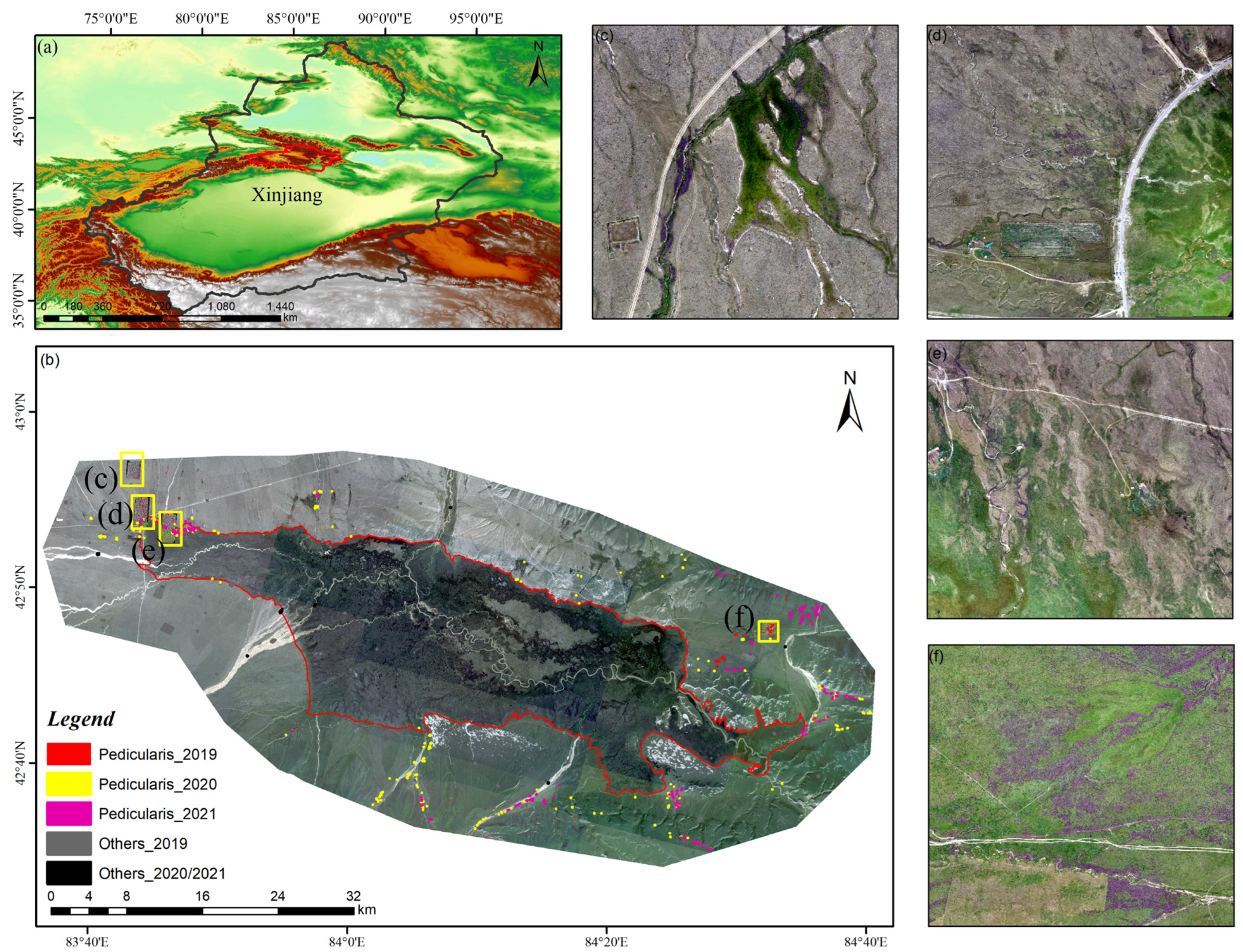
All calculations and analyses of the research were performed in Python (v3.6.12) and the geographic information system ArcGIS (v10.6, ESRI). The experiment was run on Windows 10 on a machine with two 36-core Intel Xeon 3.10 GHz processors and 128 GB RAM. The technology workflow of the study has been organized in the following sections (Figure 1).

2.1. Study Area

The Bayinbuluke Grassland (42°18′~43°34′N, 82°27′~86°17′E), in the southern hinterland of the central part of Mountain Tianshan, is located in the northwest region of Hejing county in Xinjiang Province [34]. Furthermore, it is the second largest grassland in China and the most extensive subalpine, alpine meadow grassland in the desert region of China, with a total area of 3523.94 km2 [35,36], and the main vegetation types are alpine grassland and swampy alpine meadows [37]. The Bayinbuluke Grassland is part of the Kaidu River basin, where water comes mainly from alpine snow melting and the recharge of natural precipitation. Its altitude is 2400~4400 m; the average annual temperature is −4.7 °C, with an extreme high of 28.3 °C and an extreme low of −48.1 °C; the annual precipitation is 216.8~361.8 mm; it experiences about 150~180 d of snow; and the annual dry grass period is seven months. Due to the cold weather, the soil in this area is frozen and there are almost no large trees. There are six main land use types in this grassland: high-cover pasture, low-cover pasture, marshland, timberland, water, and wild land. The water areas include rivers and lakes in the grassland and mountain snowfields [34]. The study area is shown in Figure 2.

2.2. Data Sources

2.2.1. UAV RGB Imagery

Selecting samples through a visual interpretation of remote sensing images with a low spatial resolution (relative to UAV images) presents a challenge due to the varying degrees of sparsity in the distribution of Pedicularis across different regions. Therefore, this study selected Pedicularis samples on satellite images via visual interpretation with the aid of UAV RGB (380~760 nm) imagery, which was obtained using a SONY RX1RII. The UAV data selected for the study area were taken on 7 August (f), 8 August (c), and 9 August (d, e), 2019 (Figure 2). The UAV was a DJI M600 (DJI, Shenzhen, China), and the flight information was planned in DJI GS Pro. The flight height of the UAV was 230 m, and the forward and side overlaps were 80% and 70%, respectively. The spatial resolution of all images acquired was 3 cm. The areas photographed by the UAV and where it was located are shown in Figure 2.

2.2.2. Sentinel-2 Imagery

The Sentinel-2 L2-level product used in the study was a Sentinel-2 Multispectral Instrument (MSI) from the European Space Agency (ESA). Sentinel-2 images cover 13 spectral bands in the visible, near-infrared (NIR), and short-wave infrared (SWIR) wavelengths, with four bands at 10 m, six bands at 20 m, and three bands at 60 m spatial resolution. The characteristics of the bands are listed in Table 1. For Sentinel-2 data, four 10 m and six 20 m bands can be used for land cover/land use (LCLU) mapping and change detection. The Sentinel-2 L2-level product provides the surface reflectance of images [38]. Regarding the matching of imaging data, imaging quality, and imaging time, through the Google Earth Engine platform, this study screened remote sensing images from 1 August to 31 August 2019. In order to obtain a better surface reflectance product, the Sentinel-2 L2-level product needs to be filtered and pre-processed. This experiment selected images with less than 10% cloudiness and filled the filtered images via temporal interpolation. Next, the filtered images were mosaicked and clipped through the region of interest (ROI) and all bands were resampled to 10 m. The sensor configuration of Sentinel-2 is as follows [39].

2.2.3. PlanetScope Imagery

The PlanetScope images with a 3 m spatial resolution were from the Planet Labs. It had four reflectance bands—blue, green, red, and near-infrared—with near-daily global coverage. The PlanetScope images can be accessed for free by researchers through a research and education license (https://developers.planet.com/ (accessed on 1 May 2022)). This study used a Level-3B surface reflectance product, which was geometrically corrected, radiometrically corrected, and atmospherically corrected. We also processed it with ENVI (v5.3, ESRI) for mosaic, registration, and reflectance calculations (divided by 10,000). The daily acquisition of PlanetScope data allowed us to select images with optimal imaging quality for our analysis. For our experiment, we selected PlanetScope images from 7 August and 12 August 2019. Similarly, for the year 2020, we selected images acquired on 5 August, 24 August, and 30 August. For the year 2021, we selected images acquired on 11 August, 18 August, and 23 August. The configuration information for the PlanetScope satellite is as Table 2 [40].

2.3. Datasets and Data Analysis

2.3.1. Generation of Additional Features

Identifying Pedicularis on satellite images is a challenging operation. It is difficult to identify Pedicularis accurately through object-oriented methods. Therefore, it is necessary to use pixel-based classification to extract Pedicularis, and feature engineering is a particularly useful method. Some work in the literature has indicated that spectral features and combined vegetation indices are more essential than textural features and principal components in target identification and classification [41,42].
In order to better extract Pedicularis from the land cover, we compared the spectral characteristics of Pedicularis and familiar grasses. These spectral curves were obtained from the results in a previous study [43]. The normalized difference vegetation index (NDVI), the normalized ratio vegetation index (RVI), and the difference water index (NDWI) were obtained using Equations (1)–(3), respectively. The NDVI is one of the most influential parameters for characterizing changes in vegetation greenness, and it is often employed in studies of land cover [44]. RVI is widely used to estimate and monitor the biomass of green plants [45]. Pedicularis is a water-loving plant, often growing next to rivers [4,46]. Therefore, this experiment calculated the NDWI to extract Pedicularis [47]. Numerous studies have verified that the three indices are efficient for land use/land cover and target extraction [44,45,48,49,50,51].
N D V I = ρ n i r ρ r e d ρ n i r + ρ r e d   ,
R V I = ρ n i r ρ r e d   ,
N D W I = ρ green ρ n i r ρ green + ρ n i r   .

2.3.2. Construction of the Datasets

This study was based on UAV RGB images from the PlanetScope and Sentinel-2 satellites, with visual interpretation using ROIs plotted on the UAV RGB images to select the Pedicularis samples. These data were obtained in August for each of the years 2019~2021, and the details are presented in Section 2.2. Subsequently, we selected a sample of non-Pedicularis species for 2019 to 2021, ensuring that the chosen locations exhibited a consistent distribution of non-Pedicularis species in 2020 and 2021. Finally, the samples used as input data for the construction of the model were of three types: PlanetScope data (7 features), Sentinel-2 data (7 features), and Sentinel-2 data (13 features). The sample information is shown in Table 3. The location of the sample selection is shown in Figure 2b.
The constructed models were applied to three different datasets for change detection in multi-period remotely sensed images. The classification results were evaluated and analyzed separately, and the samples were partitioned into training and test sets at an 8:2 ratio. To ensure balance within the training set, we performed downsampling such that the proportion of positive class samples to unlabeled samples was 3:7 in 2020/2021. Since the sample size in 2019 was sufficient, 1:1 was chosen for modelling to ensure the model’s generalizability. The details of the selected samples are shown in Table 3.

2.4. Methodology

2.4.1. Classification Method

This study used the PUL method, which was demonstrated to be feasible for identifying Pedicularis in another study [21]. This method is based on the bootstrap aggregation (bagging) technique: the algorithm iteratively trains many binary classifiers to distinguish known positive (P) examples from random subsamples of the unlabeled (U) dataset and to average their predictions. PUL is a semi-supervised learning algorithm based on a positive and unlabeled sample [52]. This study chose decision trees as the base classifiers and described PUL’s classification results in detail. Similar to all machine learning approaches, the PUL methodology encounters challenges in addressing the intricacies of spatiotemporal migration within the recognition process. However, this algorithm is a few-shot learning approach, which is well-suited for addressing the challenge of identifying Pedicularis in the presence of limited samples, particularly within a vast spatial extent.
The steps are as follows: (1) determine a set of reliable negation (RN) examples, which has a small number of positive samples, from U and transform the problem into a binary classification problem; (2) train binary classifiers based on P and RN by iteratively applying existing classification algorithms; and (3) iterate over the previous two steps, with the number of bootstrap samples T also being a user-defined parameter. Finally, the probability of each unlabeled sample being judged as a positive sample is calculated.
In the PUL classifier, positive and negative samples are selected from the training dataset to train the model. In an example conducted in 2019, Sentinel-2 had 7690 positive and 7690 negative samples. To improve the training efficiency of PUL, we trained ‘n’ decision trees to fit the training dataset. Firstly, we selected 10% of the positive class samples as positive samples (y = 1); secondly, the remaining 90% of positive class samples and all negative class samples were labeled as unlabeled samples (y = 0); then, the same proportion of unlabeled samples was randomly selected as negative samples (y = −1) for training; and, finally, ‘k’ iterations were performed in this manner. The probability of each sample being positive was calculated to obtain the classification result of this classifier. The parameter ‘k’ was adjusted from 100 to 2000 with a step size of 100. The ‘n’ ranged from 100 to 1000 with a step size of 100. PlanetScope datasets were modelled using the same methodology and range of parameters.

2.4.2. Accuracy Assessment

Using PUL, we obtained a confusion matrix and calculated the evaluation metrics on the test dataset, including recall, precision, overall accuracy (OA), F1-score, and AUC (area under the ROC curve), which can be calculated using the ROC curve (receiver operating characteristic curve). These metrics were utilized to assess the model’s performance. Precision represents predictions for a positive class in the truly labeled dataset and can be obtained using Equation (4). Recall represents the evaluation of samples predicted to be in the positive class and can be obtained using Equation (5). Overall accuracy (OA) is the sum of the true positives plus true negatives divided by the total number of tested individuals, as shown in Equation (7). F1-score is a metric that combines the strengths of precision and recall, is well suited for evaluating models in situations where there is an imbalance between categories, and can be calculated using Equation (8). AUC can be viewed as the probability of randomly selecting a pair of positive and negative samples from a sample, which is the area under the ROC curve drawn using the FPR and TPR (Equations (5) and (6)). The AUC is less sensitive to class imbalance than OA and reflects the model’s performance under sample imbalance more accurately [53].
p r e c i s i o n = T P T P + F P   ,
T P R = r e c a l l = T P T P + F N   ,
F P R = F P T N + F P .
O A = T P + T N T P + T N + F P + F N   ,
F 1 s c o r e = 2 × p r e c i s i o n × r e c a l l p r e c i s i o n + r e c a l l
TP, FP, FN, and TN are the classifications true positive, false positive, false negative, and true negative, respectively.

2.4.3. Change Detection

This study took the distribution area and proportion, and the change rate of Pedicularis from the classification results for 2019–2021 [54]. To further reflect the direction, amount, and rate of Pedicularis change, this study generated a dynamic transfer matrix from the change detection results in 2019–2021, which can reflect the flow of species change [55]. Based on these results, we analyzed the change in the dynamics of Pedicularis. The change rate of the area of Pedicularis was calculated using Equation (8).
C i = W b i W a i W a i × 1 t × 100 %   .
where C i is the change rate of Pedicularis during the study period; W a i and W b i are the distribution areas of Pedicularis at the beginning and end of the study period, respectively; t is the study period, measured by year; and the calculation results indicate the annual change rate of Pedicularis [56].
A transfer matrix model can depict a species’ evolutionary patterns, capturing both species distribution changes and their migration directions. Using the classification outcomes of the study area in 2019, 2020, and 2021, we derived the transfer areas for each stage and constructed a transfer matrix.
S i j = [ S 11 S 1 n S n 1 S n n ]   .
where S is the species area; i and j are the species types at the beginning and end of the study, respectively; and n is the number of species types.

3. Results

3.1. Comparison of Classification Accuracy on Sentinel-2 and PlanetScope

Three classifiers were developed for the positive and unlabeled learning (PUL) method using three different types of datasets. Based on the results presented in Table 4, the highest extraction accuracy for Pedicularis was observed when using Sentinel-2 data (13 features), yielding an F1-score of 0.9405. On the other hand, the lowest classification accuracy was obtained using PlanetScope data, resulting in an F1-score of 0.7049. Notably, the classification accuracy for Pedicularis using Sentinel-2 data (7 features) was significantly higher compared with that obtained using PlanetScope data and slightly lower than the accuracy observed for Sentinel-2 data (13 features).
Our findings indicate that the highest classification accuracy for Pedicularis was observed in 2019. While recall and precision were generally comparable across most models, recall was found to be higher than precision for the models built using PlanetScope data. Moreover, our results demonstrate that the difference between accuracy and F1-score is minimal when the model’s accuracy is high but becomes more pronounced when the accuracy is low.
To evaluate the temporal transferability of the model, we tested the model developed in 2019 on data from 2020 and 2021. As illustrated in Figure 3, the model’s performance on this test was unsatisfactory, with the F1-scores for both years being less than 0.62. Specifically, the F1-score for the PlanetScope dataset in 2020 was insufficient, with a value of only 0.3300. Subsequently, upon training the model with the corresponding year’s training set, a notable improvement in accuracy was observed. These results demonstrate the potential of positive and unlabeled learning (PUL) for small-sample learning.
As evidenced by the ROC and AUC curves depicted in Figure 4, changes in precision and recall exhibit an inverse relationship while the AUC values remain stable. In order to maximize the AUC, we could appropriately adjust the threshold to manipulate the precision and recall, ultimately achieving a balance between the two for accurate classification of Pedicularis. However, in scenarios with a large F1-score and accuracy gap, the AUC of the model remains low compared with that of other models.

3.2. Changes in Dynamics of Pedicularis

The classification results obtained using Sentinel-2 data (13 features) were the most accurate among all models. Accordingly, changes in the distribution area of Pedicularis from 2019 to 2021 were monitored based on this classification result. The analysis revealed that Pedicularis had the largest area, 195.7803 km2, in 2019, accounting for 5.55% of the total region, while its size decreased to 3.54% in 2020.
Figure 5 illustrates the spatiotemporal distribution of Pedicularis from 2019 to 2021 using Sentinel-2 data (13 features). The results showed a gradual decrease in its distribution in the northwest and an increase in the south over the past three years. Additionally, the total distribution area of Pedicularis showed a decreasing and then increasing trend over this period.
The change in the distribution area of Pedicularis in the Bayinbuluke Grassland was analyzed from 2019 to 2021. Comparing the changes in Pedicularis in 2019 and 2020, it was observed that 173.89 km2 of the Pedicularis distribution area disappeared, while 103.0704 km2 was converted from distribution areas of other species to that of Pedicularis, indicating an overall improvement. From 2020 to 2021, there was a decrease of 106.0108 km2 in Pedicularis, followed by an increase of 138.2587 km2. However, the total amount of Pedicularis from 2019 to 2021 still decreased, with a decrease in distribution area of 38.5740 km2.

4. Discussion

4.1. Influencing Factors of Classification Accuracy

We can identify Pedicularis clearly from the high-resolution drone images. However, the low spatial resolution of the images and the interplay of spectral information from different land covers produce mixed pixels. These phenomena result in the color and geometric textural information of Pedicularis not being easily acquired on satellite images. The PUL method used in this study can effectively improve the classification accuracy of Pedicularis based on satellite imagery; relevant studies on UAV imagery can support this method [21].
During the mosaicking of data, an uneven color balance across multiple images can have an impact on the outcome of image classification [57]. Sentinel-2 only requires two images to be sufficient to cover the study area; PlanetScope has a higher temporal resolution and a smaller coverage area per image. It requires 41 images to cover the study area, making the classifier more likely to learn some noise.
The accuracy of Pedicularis extraction was significantly enhanced by increasing the number of features from 7 to 13 in the Sentinel-2 classification results. This finding aligns with other pixel-based classification methods [58]. Moreover, the classification results of the model constructed using Sentinel-2 data (13 features) provide a more realistic distribution of Pedicularis.
Comparing the identification results of PlanetScope data (seven features) and Sentinel-2 data (seven features), the identification result for the 10 m resolution is higher than that for the 3 m resolution, which is unexpected. Our analysis shows that this is mainly caused by the significant difference in spectral reflectance between the images due to PlanetScope requiring more images [59,60]. Additionally, the band characteristics of the pixels are contingent on the complexity of the species within each pixel: the more intricate the object within the pixel, the greater the divergence between its spectral features and the pure pixel features, resulting in the reduced recognition accuracy of scattered patterns. Conversely, during sample selection, we noticed that Pedicularis was easier to identify in Sentinel-2 images compared to PlanetScope images, based solely on color considerations.
It has been found that the spectral signature of the same object using the same sensor may vary at different times, and this phenomenon also affects the classification results. Consequently, identifying features resistant to temporal and spectral variations is crucial for pixel-based classification methods, and can also help to improve the reliability of monitoring changes after classification.

4.2. Spatiotemporal Pattern of Pedicularis

Figure 5, Table 5 and Table 6 collectively elucidate the dynamic trajectory of the spatial distribution of Pedicularis and characterize its temporal pattern, marked by an initial decrease, followed by a subsequent increase from 2019 to 2021. While the distribution of Pedicularis sharply decreased in the northwestern region between 2019 and 2020, other regions showed no significant migration trend. Furthermore, in 2021, the distribution area of Pedicularis in the southern region showed an increasing trend. As depicted in Figure 5, the distribution of Pedicularis was predominantly along rivers, suggesting that Pedicularis is a water-loving plant, which is consistent with local investigation findings [43]. Following a comprehensive survey, it has been observed that the precipitation levels in the region have exhibited a decline from 2019 to 2020. This observation explains the decrease also seen in the distribution of Artemisia marcescens [61]. This case also contributes to the investigation into the driving mechanisms underlying Pedicularis distribution. By utilizing GIS methods to analyze the spatial distribution of Pedicularis, a further understanding of its invasion routes and drivers can be attained.
This article discusses the feasibility of a spatiotemporal analysis based on PlanetScope and Sentinel-2 imagery. Both satellites have a high temporal resolution and meet the needs of long-time-series monitoring. However, post-classification change monitoring can avoid influencing the classification results due to different spatiotemporal and data sources. The accuracy of the classification results dramatically affects the detection of changes in the distribution of Pedicularis. It further shows that investigating a classifier or feature factor that can resist spatial and temporal variation and developing a better transfer learning method are essential.

4.3. A Case of Pedicularis Eradication

We learned that the government conducted a local campaign for the removal of Pedicularis in July 2019. To verify the process of eliminating Pedicularis, we looked up remote sensing images from PlanetScope, which has a high spatial resolution, for July 2019. These images correspond to the position in Figure 2f. As seen from Figure 6, Pedicularis was physically removed by local people on 17 July, 23 July, and 29 July 2019. It is, therefore, essential to identify the location of Pedicularis and its dynamics. This contributes to the local government’s efforts to control the invasion of Pedicularis and to protect the ecological environment [1,7].

5. Conclusions

The main contribution of this work is the use of a new PUL method to extract Pedicularis. This extracted Pedicularis distribution is subsequently employed for the dynamic detection of Pedicularis and for conducting a spatiotemporal analysis of the prediction results. With the use of the spatial distribution of Pedicularis from 2019 to 2021, we can achieve real-time monitoring and the effective eradication of Pedicularis. In contrast to the one-class classifier, which only uses positive-class samples, PUL makes full use of numerous unlabeled samples to improve the accuracy of the classification results, contributing to curbing the expansion of the distribution area of poisonous Pedicularis. The conclusions are as follows:
(1)
The proliferation of Pedicularis in the Bayinbuluke Grassland has resulted in significant ecological damage, necessitating the substantial expenditure of resources and efforts by the provincial government for rehabilitation efforts. In addressing this issue, change-detection methods utilizing remote sensing technology offer a practical approach for informed management and mitigation. Sentinel-2 images have the advantages of a large width, easily acquirable data, and high accuracy in extracting Pedicularis. The resolution of PlanetScope is higher than that of Sentinel-2, which is more advantageous when removing Pedicularis from small areas. The results of the study show that the PUL method is able to achieve a high recognition accuracy across different images.
(2)
Within the confines of the same sensor platform, the influence of feature count on improvements to the identification accuracy becomes obvious with an ample sample size, as evidenced by an increasing feature count coinciding with increased recognition accuracy. However, within an equivalent feature framework, the correlation between resolution elevation and accuracy enhancement does not invariably hold, implying that the resultant classification outcome is dependent on the inherent data quality obtained using the sensor apparatus.
(3)
The post-classification comparison algorithm avoids spectral differences in remote sensing images, especially long-time-series images from different sensors. It enables the rapid monitoring of regional variations in the distribution of different land types. However, it is highly dependent on the stability of the model, and a transferred, high-accuracy classification model needs to be further developed. The distribution of Pedicularis is concentrated in the northwestern and southwestern parts of Bayinbuluke Swan Lake. From 2019 to 2021, the distribution area of Pedicularis exhibited a fluctuating trend, initially increasing and then subsequently decreasing, with the 2021 area measuring 157.2063 km2. Despite better eradication efforts in the northeast region, the distribution area of Pedicularis did not exhibit significant changes, indicating that grassland managers may not have done enough to control the growth of Pedicularis.

Author Contributions

Methodology: W.W. and J.T.; validation: W.W., J.T. and N.Z.; formal analysis: W.W.; investigation: N.Z., Y.W. and J.T.; writing—original draft preparation: W.W.; writing—review and editing: W.W., J.T., X.X. and A.Z.; N.Z. contributed the same as the corresponding authors. All authors have read and agreed to the published version of the manuscript.

Funding

This research was funded by the Strategic Priority Research Program of the Chinese Academy of Sciences (XDA20050103) and the National Key Research and Development Program of China (No. 2020YFC1807102).

Data Availability Statement

Not applicable.

Conflicts of Interest

The authors declare no conflict of interest.

References

  1. Fu, P.; Yao, J.; Hu, J.; Guo, X. Capital Endowments, Policy Perceptions and Herdsmen’s Willingness to Reduce Livestock:A Case Study from the World Natural Heritage Site of Bayinbuluke. Acta Agrestia Sin. 2021, 29, 780–787. [Google Scholar]
  2. Hameed, A.; Zafar, M.; Ahmad, M.; Sultana, S.; Bahadur, S.; Anjum, F.; Shuaib, M.; Taj, S.; Irm, M.; Altaf, M.A. Chemo-taxonomic and biological potential of highly therapeutic plant Pedicularis groenlandica Retz. using multiple microscopic techniques. Microsc. Res. Tech. 2021, 84, 2890–2905. [Google Scholar] [CrossRef] [PubMed]
  3. Elkind, K.; Sankey, T.T.; Munson, S.M.; Aslan, C.E. Invasive buffelgrass detection using high-resolution satellite and UAV imagery on Google Earth Engine. Remote Sens. Ecol. Conserv. 2019, 5, 318–331. [Google Scholar] [CrossRef]
  4. Sui, X.; Li, A.; Guan, K. Impacts of climatic changes as well as seed germination characteristics on the population expansion of Pedicularis verticillata. Ecol. Environ. Sci. 2013, 22, 1099–1104. [Google Scholar]
  5. Yanyan, L.I.U.; Yukun, H.U.; Jianmei, Y.U.; Kaihui, L.I.; Guogang, G.A.O.; Xin, W. Study on Harmfulness of Pedicularis myriophylla and Its Control Measures. Arid Zone Res. 2008, 25, 778–782. [Google Scholar]
  6. Hongtao, J.I.A.; Pingan, J.; Luming, C.; Chengyi, Z.; Yukun, H.U. Estimation of Organic Carbon Storage of Bayinbuluke Alpine Grassland Ecosystem. Xinjiang Agric. Sci. 2006, 43, 480–483. [Google Scholar]
  7. Pingan, J.; Hui, L.I.; Hongtao, J.I.A.; Zihong, D. Impacts of fencing on soil animals diversity beneath mountainous lawn vegetation in Bayinbuluke. J. Northwest Sci-Tech Univ. Agric. For. 2007, 35, 69–74. [Google Scholar]
  8. Choudhary, K.; Boori, M.S.; Kupriyanov, A. Landscape Analysis through Remote Sensing and GIS Techniques: A Case Study of Astrakhan, Russia. In Proceedings of the 8th International Conference on Graphic and Image Processing (ICGIP), Tokyo, Japan, 29–31 October 2016. [Google Scholar]
  9. Gao, S.; Zheng, J.; Ma, T.; Wu, J.; Nasongcaoketu; Maidi, K. Research on the Applicability of Remote Sensing Monitoring of Inedible Grass Pedicularis sp. by GF-1 WFV Satellite in Bayanbulak Grassland. Xinjiang Agric. Sci. 2017, 54, 1949–1956. [Google Scholar]
  10. Huber, N.; Ginzler, C.; Pazur, R.; Descombes, P.; Baltensweiler, A.; Ecker, K.; Meier, E.; Price, B. Countrywide classification of permanent grassland habitats at high spatial resolution. Remote Sens. Ecol. Conserv. 2023, 9, 133–151. [Google Scholar] [CrossRef]
  11. Lopatin, J.; Dolos, K.; Kattenborn, T.; Fassnacht, F.E. How canopy shadow affects invasive plant species classification in high spatial resolution remote sensing. Remote Sens. Ecol. Conserv. 2019, 5, 302–317. [Google Scholar] [CrossRef]
  12. Kakembo, V.; Smith, J.; Kerley, G. A Temporal Analysis of Elephant-Induced Thicket Degradation in Addo Elephant National Park, Eastern Cape, South Africa. Rangel. Ecol. Manag. 2015, 68, 461–469. [Google Scholar] [CrossRef]
  13. Singh, P.S.; Singh, V.P.; Pandey, M.K.; Karthikeyan, S.; IEEE. One-class Classifier Ensemble based Enhanced Semisupervised Classification of Hyperspectral Remote Sensing Images. In Proceedings of the 2nd IEEE International Conference on Emerging Smart Computing and Informatics (ESCI), All India Shri Shivaji Memorial Soc, Inst Informat Technol, Pune, India, 12–14 March 2020; pp. 22–27. [Google Scholar]
  14. Hossain, M.A.; Jia, X.; Benediktsson, J.A. One-Class Oriented Feature Selection and Classification of Heterogeneous Remote Sensing Images. IEEE J. Sel. Top. Appl. Earth Obs. Remote Sens. 2016, 9, 1606–1612. [Google Scholar] [CrossRef]
  15. Li, W.; Guo, Q.; Elkan, C. A Positive and Unlabeled Learning Algorithm for One-Class Classification of Remote-Sensing Data. IEEE Trans. Geosci. Remote Sens. 2011, 49, 717–725. [Google Scholar] [CrossRef]
  16. Mack, B.; Roscher, R.; Waske, B. Can I Trust My One-Class Classification? Remote Sens. 2014, 6, 8779–8802. [Google Scholar] [CrossRef]
  17. Li, W.K.; Guo, Q.H. A maximum entropy approach to one-class classification of remote sensing imagery. Int. J. Remote Sens. 2010, 31, 2227–2235. [Google Scholar] [CrossRef]
  18. Braun, A.C. Evaluation of One-Class Svm for Pixel-Based and Segment-Based Classification in Remote Sensing. In Proceedings of the ISPRS-Technical-Commission III Symposium on Photogrammetric Computer Vision and Image Analysis (PCV), Saint Mande, France, 1–3 September 2010; pp. 160–165. [Google Scholar]
  19. Chang, S.; Du, B.; Zhang, L. A Subspace Selection-Based Discriminative Forest Method for Hyperspectral Anomaly Detection. IEEE Trans. Geosci. Remote Sens. 2020, 58, 4033–4046. [Google Scholar] [CrossRef]
  20. Dambros, C.S.; Morais, J.W.; Azevedo, R.A.; Gotelli, N.J. Isolation by distance, not rivers, control the distribution of termite species in the Amazonian rain forest. Ecography 2017, 40, 1242–1250. [Google Scholar] [CrossRef]
  21. Wang, W.; Tang, J.; Zhang, N.; Xu, X.; Zhang, A.; Wang, Y. Automated Detection Method to Extract Pedicularis Based on UAV Images. Drones 2022, 6, 399. [Google Scholar] [CrossRef]
  22. Morshed, N.; Yorke, C.; Zhang, Q. Urban Expansion Pattern and Land Use Dynamics in Dhaka, 1989–2014. Prof. Geogr. 2017, 69, 396–411. [Google Scholar] [CrossRef]
  23. Franklin, S.E.; Ahmed, O.S.; Wulder, M.A.; White, J.C.; Hermosilla, T.; Coops, N.C. Large Area Mapping of Annual Land Cover Dynamics Using Multitemporal Change Detection and Classification of Landsat Time Series Data. Can. J. Remote Sens. 2015, 41, 293–314. [Google Scholar] [CrossRef]
  24. Angulo, D.; Angulo, F.; Olivar, G. Dynamics and Forecast in a Simple Model of Sustainable Development for Rural Populations. Bull. Math. Biol. 2015, 77, 368–389. [Google Scholar] [CrossRef] [PubMed]
  25. Wu, T.J.; Luo, J.C.; Zhou, Y.N.; Wang, C.P.; Xi, J.B.; Fang, J.W. Geo-Object-Based Land Cover Map Update for High-Spatial-Resolution Remote Sensing Images via Change Detection and Label Transfer. Remote Sens. 2020, 12, 174. [Google Scholar] [CrossRef]
  26. Yu, W.J.; Zhou, W.Q.; Qian, Y.G.; Yan, J.L. A new approach for land cover classification and change analysis: Integrating backdating and an object-based method. Remote Sens. Environ. 2016, 177, 37–47. [Google Scholar] [CrossRef]
  27. Chen, X.H.; Chen, J.; Shi, Y.S.; Yamaguchi, Y. An automated approach for updating land cover maps based on integrated change detection and classification methods. ISPRS-J. Photogramm. Remote Sens. 2012, 71, 86–95. [Google Scholar] [CrossRef]
  28. Qian, Y.G.; Zhou, W.Q.; Yu, W.J.; Han, L.J.; Li, W.F.; Zhao, W.H. Integrating Backdating and Transfer Learning in an Object-Based Framework for High Resolution Image Classification and Change Analysis. Remote Sens. 2020, 12, 4094. [Google Scholar] [CrossRef]
  29. Xu, Y.D.; Yu, L.; Zhao, F.R.; Cai, X.L.; Zhao, J.Y.; Lu, H.; Gong, P. Tracking annual cropland changes from 1984 to 2016 using time-series Landsat images with a change-detection and post-classification approach: Experiments from three sites in Africa. Remote Sens. Environ. 2018, 218, 13–31. [Google Scholar] [CrossRef]
  30. Feng, X.; Li, P.; Cheng, T. Detection of Urban Built-Up Area Change From Sentinel-2 Images Using Multiband Temporal Texture and One-Class Random Forest. IEEE J. Sel. Top. Appl. Earth Obs. Remote Sens. 2021, 14, 6974–6986. [Google Scholar] [CrossRef]
  31. Kempeneers, P.; Sedano, F.; Strobl, P.; McInerney, D.O.; San-Miguel-Ayanz, J. Increasing Robustness of Postclassification Change Detection Using Time Series of Land Cover Maps. IEEE Trans. Geosci. Remote Sens. 2012, 50, 3327–3339. [Google Scholar] [CrossRef]
  32. Crowson, M.; Hagensieker, R.; Waske, B. Mapping land cover change in northern Brazil with limited training data. Int. J. Appl. Earth Obs. Geoinf. 2019, 78, 202–214. [Google Scholar] [CrossRef]
  33. Colditz, R.R.; Acosta-Velazquez, J.; Diaz Gallegos, J.R.; Vazquez Lule, A.D.; Teresa Rodriguez-Zuniga, M.; Maeda, P.; Cruz Lopez, M.I.; Ressl, R. Potential effects in multi-resolution post-classification change detection. Int. J. Remote Sens. 2012, 33, 6426–6445. [Google Scholar] [CrossRef]
  34. Bao, A.; Cao, X.; Chen, X.; Xia, Y. Study on Models for Monitoring of Aboveground Biomass about Bayinbuluke grassland Assisted by Remote Sensing. In Proceedings of the Conference on Remote Sensing and Modeling of Ecosystems for Sustainability, San Diego, CA, USA, 13 August 2008. [Google Scholar]
  35. Chen, X.; Yang, Z.; Wang, T.; Han, F. Landscape Ecological Risk and Ecological Security Pattern Construction in World Natural Heritage Sites: A Case Study of Bayinbuluke, Xinjiang, China. ISPRS Int. J. Geo-Inf. 2022, 11, 328. [Google Scholar] [CrossRef]
  36. Xu, X.; Wang, X.; Zhu, X.; Jia, H.; Han, D. Landscape Pattern Changes in AlpineWetland of Bayanbulak Swan Lake during 1996–2015. J. Nat. Resour. 2018, 33, 1897–1911. [Google Scholar]
  37. Liu, Q.; Yang, Z.P.; Han, F.; Shi, H.; Wang, Z.; Chen, X.D. Ecological Environment Assessment in World Natural Heritage Site Based on Remote-Sensing Data. A Case Study from the Bayinbuluke. Sustainability 2019, 11, 6385. [Google Scholar] [CrossRef]
  38. Grabska, E.; Frantz, D.; Ostapowicz, K. Evaluation of machine learning algorithms for forest stand species mapping using Sentinel-2 imagery and environmental data in the Polish Carpathians. Remote Sens. Environ. 2020, 251, 112103. [Google Scholar] [CrossRef]
  39. De Vroey, M.; de Vendictis, L.; Zavagli, M.; Bontemps, S.; Heymans, D.; Radoux, J.; Koetz, B.; Defourny, P. Mowing detection using Sentinel-1 and Sentinel-2 time series for large scale grassland monitoring. Remote Sens. Environ. 2022, 280, 113145. [Google Scholar] [CrossRef]
  40. Kimm, H.; Guan, K.Y.; Jiang, C.Y.; Peng, B.; Gentry, L.F.; Wilkin, S.C.; Wang, S.B.; Cai, Y.P.; Bernacchi, C.J.; Peng, J.; et al. Deriving high-spatiotemporal-resolution leaf area index for agroecosystems in the US Corn Belt using Planet Labs CubeSat and STAIR fusion data. Remote Sens. Environ. 2020, 239, 111615. [Google Scholar] [CrossRef]
  41. Holloway-Brown, J.; Helmstedt, K.J.; Mengersen, K.L. Interpolating missing land cover data using stochastic spatial random forests for improved change detection. Remote Sens. Ecol. Conserv. 2021, 7, 649–665. [Google Scholar] [CrossRef]
  42. Saber, A.; El-Sayed, I.; Rabah, M.; Selim, M. Evaluating change detection techniques using remote sensing data: Case study New Administrative Capital Egypt. Egypt. J. Remote Sens. Space Sci. 2021, 24, 635–648. [Google Scholar] [CrossRef]
  43. Gao, S.; Lin, J.; Ma, T.; Wu, J.; Zheng, J. Extraction and Analysis of Hyperspectral Data and Characteristics fromPedicularis on Bayanbulak Grassland in Xinjiang. Remote Sens. Technol. Appl. 2018, 33, 908–914. [Google Scholar]
  44. Carlson, T.N.; Ripley, D.A. On the relation between NDVI, fractional vegetation cover, and leaf area index. Remote Sens. Environ. 1997, 62, 241–252. [Google Scholar] [CrossRef]
  45. Gnyp, M.L.; Miao, Y.X.; Yuan, F.; Ustin, S.L.; Yu, K.; Yao, Y.K.; Huang, S.Y.; Bareth, G. Hyperspectral canopy sensing of paddy rice aboveground biomass at different growth stages. Field Crops Res. 2014, 155, 42–55. [Google Scholar] [CrossRef]
  46. Wang, D.; Cui, B.C.; Duan, S.S.; Chen, J.J.; Fan, H.; Lu, B.B.; Zheng, J.H. Moving north in China: The habitat of Pedicularis kansuensis in the context of climate change. Sci. Total Environ. 2019, 697, 133979. [Google Scholar] [CrossRef] [PubMed]
  47. Chai, L.; Jiang, H.; Crow, W.T.; Liu, S.; Zhao, S.; Liu, J.; Yang, S. Estimating Corn Canopy Water Content From Normalized Difference Water Index (NDWI): An Optimized NDWI-Based Scheme and Its Feasibility for Retrieving Corn VWC. IEEE Trans. Geosci. Remote Sens. 2021, 59, 8168–8181. [Google Scholar] [CrossRef]
  48. Francini, S.; McRoberts, R.E.; Giannetti, F.; Mencucci, M.; Marchetti, M.; Mugnozza, G.S.; Chirici, G. Near-real time forest change detection using PlanetScope imagery. Eur. J. Remote Sens. 2020, 53, 233–244. [Google Scholar] [CrossRef]
  49. Sui, Y.; Shao, F.; Wang, C.; Sun, R.; Ji, J. Complex network modeling of spectral remotely sensed imagery: A case study of massive green algae blooms detection based on MODIS data. Phys. A-Stat. Mech. Its Appl. 2016, 464, 138–148. [Google Scholar] [CrossRef]
  50. Zhao, B.; Yang, F.; Zhang, R.; Shen, J.; Pilz, J.; Zhang, D. Application of unsupervised learning of finite mixture models in ASTER VNIR data-driven land use classification. J. Spat. Sci. 2021, 66, 89–112. [Google Scholar] [CrossRef]
  51. Zhou, X.-X.; Li, Y.-Y.; Luo, Y.-K.; Sun, Y.-W.; Su, Y.-J.; Tan, C.-W.; Liu, Y.-J. Research on remote sensing classification of fruit trees based on Sentinel-2 multi-temporal imageries. Sci. Rep. 2022, 12, 11549. [Google Scholar] [CrossRef]
  52. Mordelet, F.; Vert, J.P. A bagging SVM to learn from positive and unlabeled examples. Pattern Recognit. Lett. 2014, 37, 201–209. [Google Scholar] [CrossRef]
  53. Halligan, S.; Altman, D.G.; Mallett, S. Disadvantages of using the area under the receiver operating characteristic curve to assess imaging tests: A discussion and proposal for an alternative approach. Eur. Radiol. 2015, 25, 932–939. [Google Scholar] [CrossRef] [PubMed]
  54. Wang, L.; Zheng, S.; Wang, X. The Spatiotemporal Changes and the Impacts of Climate Factors on Grassland in the Northern Songnen Plain (China). Sustainability 2021, 13, 6568. [Google Scholar] [CrossRef]
  55. Zhang, Z.; Yang, X.; Xie, F. Macro analysis of spatiotemporal variations in ecosystems from 1996 to 2016 in Xishuangbanna in Southwest China. Environ. Sci. Pollut. Res. 2021, 28, 40192–40202. [Google Scholar] [CrossRef] [PubMed]
  56. Cao, Y.; Kong, L.; Ouyang, Z. Characteristics and Driving Mechanism of Regional Ecosystem Assets Change in the Process of Rapid Urbanization—A Case Study of the Beijing–Tianjin–Hebei Urban Agglomeration. Remote Sens. 2022, 14, 5747. [Google Scholar] [CrossRef]
  57. Fan, C.; Chen, X.; Zhong, L.; Zhou, M.; Shi, Y.; Duan, Y. Improved Wallis Dodging Algorithm for Large-Scale Super-Resolution Reconstruction Remote Sensing Images. Sensors 2017, 17, 623. [Google Scholar] [CrossRef] [PubMed]
  58. Zhao, L.; Li, Q.; Zhang, Y.; Wang, H.; Du, X. Normalized NDVI valley area index (NNVAI)-based framework for quantitative and timely monitoring of winter wheat frost damage on the Huang-Huai-Hai Plain, China. Agric. Ecosyst. Environ. 2020, 292, 106793. [Google Scholar] [CrossRef]
  59. Zhao, Y.; Liu, D. A robust and adaptive spatial-spectral fusion model for PlanetScope and Sentinel-2 imagery. Gisci. Remote Sens. 2022, 59, 520–546. [Google Scholar] [CrossRef]
  60. Ye, N.; Morgenroth, J.; Xu, C.; Chen, N. Indigenous forest classification in New Zealand-A comparison of classifiers and sensors. Int. J. Appl. Earth Obs. Geoinf. 2021, 102, 102395. [Google Scholar] [CrossRef]
  61. Wang, Q.; Zhai, P.-M.; Qin, D.-H. New perspectives on ‘warming–wetting’trend in Xinjiang, China. Adv. Clim. Chang. Res. 2020, 11, 252–260. [Google Scholar] [CrossRef]
Figure 1. The technology workflow of the study (Blue arrows refer to the components of Samples).
Remotesensing 15 04383 g001
Figure 2. Location of the study area. (a) The study area is located in Hejing County, Xinjiang Province, China. (b) The Swan Lake (red boundary) and its buffer zone in the Bayinbuluke Grassland (background: an RGB remote sensing image acquired from PlanetScope in August 2019). (cf) Ortho-mosaic image taken via an RGB UAV in August 2019 (the purple pixels are Pedicularis).
Remotesensing 15 04383 g002
Figure 3. Comparison of accuracy between the 2019 model and model built in the same year as the test set.
Remotesensing 15 04383 g003
Figure 4. ROC and AUC curves for the models developed from 2019 to 2021.
Remotesensing 15 04383 g004
Figure 5. Spatiotemporal pattern of Pedicularis in 2019–2021 using Sentinel-2 data (13 feature).
Remotesensing 15 04383 g005
Figure 6. Local variations in Pedicularis in PlanetScope images from July 2019 within the red box. (ac) refer to PlanetScope images taken on 17 July, 23 July, and 29 July 2019. (the purple pixels are Pedicularis).
Remotesensing 15 04383 g006
Table 1. Configuration information for the Sentinel-2 satellite.
Band NameSentinel-2A/Sentinel-2B
Central Wavelength (nm)
Resolution
(Meters)
Band 1—Coastal aerosol443.9/442.260
Band 2—Blue496.6/492.110
Band 3—Green560.0/559.010
Band 4—Red664.5/664.910
Band 5—Vegetation red edge703.9/703.820
Band 6—Vegetation red edge740.2/739.120
Band 7—Vegetation red edge782.5/779.720
Band 8—NIR835.1/832.910
Band 8A—Narrow NIR864.8/864.020
Band 9—Water Vapor945.0/943.260
Band 10—SWIR–Cirrus1373.5/1376.960
Band 11—SWIR1613.7/1610.420
Band 12—SWIR2202.4/2185.720
The 60 m spatial resolution bands were not used in the experiment.
Table 2. Configuration information for the PlanetScope satellite.
Band NameSpatial Resolution (m)Spectral Wavelength (nm)
Blue3.0464–517
Green547–585
Red650–682
NIR846–888
Table 3. Ground sample information for the study regions.
Training Samples (Pixels)Test Samples (Pixels)
PedicularisOthersPedicularisOthers
2019Sentinel-2 data (7/13 features)7690769019235598
PlanetScope data (7 features)62,06362,06315,515455,615
2020Sentinel-2 data (7/13 features)194364774861900
PlanetScope data (7 features)15,56851,89315,51515,434
2021Sentinel-2 data (7/13 features)239579835991900
PlanetScope data (7 features)19,52065,066488015,434
Others: unlabeled samples. Seven features: four 10 m bands and three vegetation indices. Thirteen features: four 10 m, six 20 m bands, and three vegetation indices.
Table 4. Assessment metrics of models during the 2019–2021 period.
YearDatasetsTypesMetrics
RecallPrecisionAccuracyF1-Score
2019Sentinel-2 data (7 features)Pedicularis0.92120.92860.96170.9248
Others0.97570.9730
Sentinel-2 data (13 features)Pedicularis0.92780.95360.97000.9405
Others0.98450.9754
PlanetScope data (7 features)Pedicularis0.84580.60420.86780.7049
Others0.87280.9610
2020Sentinel-2 data (7 features)Pedicularis0.88610.73070.91690.8009
Others0.92410.9721
Sentinel-2 data (13 features)Pedicularis0.87100.90450.95830.8874
Others0.97860.9702
PlanetScope data (7 features)Pedicularis0.83400.61320.87080.7067
Others0.87930.9584
2021Sentinel-2 data (7 features)Pedicularis0.89710.86290.94540.8796
Others0.95910.9703
Sentinel-2 data (13 features)Pedicularis0.88640.92770.95930.9065
Others0.98020.9678
PlanetScope data (7 features)Pedicularis0.89850.73990.93130.8115
Others0.93770.9791
Table 5. Statistics of distribution area of Pedicularis in different periods using Sentinel-2 data (13 features).
YearArea (km2)Area Ratio (%)
2019195.78035.55%
2020124.95843.54%
2021157.20634.46%
Table 6. Transition matrix of land cover change for 2019~2021.
2019–20202020–20212019–2021
PedicularisOthersPedicularisOthersPedicularisOthers
Pedicularis21.8880173.892318.9476106.010833.6437162.1330
Others103.07043225.0944138.25873260.7280123.55903204.6058
Disclaimer/Publisher’s Note: The statements, opinions and data contained in all publications are solely those of the individual author(s) and contributor(s) and not of MDPI and/or the editor(s). MDPI and/or the editor(s) disclaim responsibility for any injury to people or property resulting from any ideas, methods, instructions or products referred to in the content.

