A Discriminative Model for Early Detection of Anthracnose in Strawberry Plants Based on Hyperspectral Imaging Technology

Abstract

Strawberry anthracnose, caused by Colletotrichum spp., is a major disease that causes tremendous damage to cultivated strawberry plants (Fragaria × ananassa Duch.). Examining and distinguishing plants potentially carrying the pathogen is one of the most effective ways to prevent and control strawberry anthracnose disease. Herein, we used this method on Colletotrichum gloeosporioides at the crown site on indoor strawberry plants and established a classification and distinguishing model based on measurement of the spectral and textural characteristics of the disease-free zone near the disease center. The results, based on the successive projection algorithm (SPA), competitive adaptive reweighted sampling (CARS), and interval random frog (IRF), extracted 5, 14, and 11 characteristic wavelengths, respectively. The SPA extracted fewer effective characteristic wavelengths, while IRF covered more information. A total of 12 dimensional texture features (TFs) were extracted from the first three minimum noise fraction (MNF) images using a grayscale co-occurrence matrix (GLCM). The combined dataset modeling of spectral and TFs performed better than single-feature modeling. The accuracy rates of the IRF + TF + BP model test set for healthy, asymptomatic, and symptomatic samples were 99.1%, 93.5%, and 94.5%, the recall rates were 100%, 94%, and 93%, and the F1 scores were 0.9955, 0.9375, and 0.9374, respectively. The total modeling time was 10.9 s, meaning that this model demonstrated the best comprehensive performance of all the constructed models. The model lays a technical foundation for the early, non-destructive detection of strawberry anthracnose.

1. Introduction

A strawberry anthracnose disease epidemic occurring throughout the strawberry growing season has become a destructive disease in strawberries all over the world. The naked eye is unable to perceive the early stages of the occurrence of strawberry anthracnose disease. Epidemic outbreak can easily occur once pathogens reach the disease emergence stage, particularly during the growth period of strawberry plants; this has become the main factor limiting strawberry production. The disease causes tremendous loss of seedlings, and latent anthracnose infection leads to the appearance of asymptomatic diseased plants. Once diseased plants are transplanted into a fertile field, the disease may accelerate, and an epidemic can occur in a disease-favorable environment, leading to the death of all of the plants [1,2,3,4,5]. This is one of the main reasons for the early death of seedlings in cultivated strawberry fields since the promotion of Fragaria × ananassa ‘Benihoppe’, especially in the last decade.

The early detection of plant diseases is the prerequisite and foundation for disease prevention. At present, the identification of strawberry anthracnose depends mainly on manual identification and laboratory polymerase chain reaction (PCR) technology. Although very experienced strawberry growers can identify symptomatic plants infected with anthracnose, not all have sufficient experience, and even the most experienced growers cannot identify asymptomatic infected plants. PCR technology can detect whether strawberry plants are infected with the anthracnose pathogen [6,7], but this technology also has many limitations: (i) only infection in the leaves [8], petioles [9], or crowns of plants [10] can be detected, and the detection object is subjected to a certain degree of damage; (ii) due to cost constraints, only sampling testing methods can be used, and samples that are automatically selected cannot be completely analyzed; (iii) the need for laboratory testing makes it difficult for strawberry practitioners to implement this practice; and (iv) the detection of this disease requires a certain amount of time, making it difficult to meet production schedule expectations. Therefore, to achieve the rapid diagnosis and detection of the asymptomatic infection of strawberry anthracnose is of great significance for the prevention and control of strawberry diseases.

Hyperspectral technology provides support for the diagnosis and detection of plant diseases [11,12,13,14,15]. Numerous reports have been published on non-destructive disease detection using hyperspectral technology, laying the technical foundations for practical application in field production [16,17,18,19,20,21]. In the process of constructing distinguishing models using hyperspectral feature information, existing researchers have studied the use of feature extraction and characteristic wavelength selection to construct a disease distinguishing model. Fazari et al. applied convolutional neural networks (CNN) and 61-band hyperspectral images to detect anthracnose in olives, achieving 85% recognition after three days of infection [22]. Gao et al. extracted six characteristic wavelengths (690, 715, 731, 1409, 1425, and 1582 nm) using the minimum absolute shrinkage and selection algorithm, and evaluated the ability of these six characteristic wavelengths to detect grape leaf roll disease using the least squares support vector machine; the classification accuracy for asymptomatic test set data in this study reached 89.93% [23]. Anna et al. used near-infrared spectroscopy technology, support vector machines, and random forest machine learning algorithms to detect rice sheath blight before symptoms of the disease appeared. The results were verified using sparse partial least squares discriminant analysis, and the overall accuracy reached 86.1% [24]. Xu et al. utilized hyperspectral technology combined with CNN to achieve the early diagnosis of wheat Fusarium head blight; the F1 score and accuracy of the test set were 0.75 and 74%, respectively [25]. These results indicate that hyperspectral imaging technology can enable the non-destructive detection of plant diseases. At present, the use of hyperspectral technology for strawberry disease detection focuses mainly on distinguishing between infected and healthy individuals [26,27,28]. The detection of asymptomatic infections in these studies is rare, since for the detection of strawberry diseases that remain in the leaf zone, anthracnose infection in the leaf zone does not directly lead to the death of the whole plant, whereas crown disease will result in plant death [29,30]. Furthermore, the above research only used universal machine learning models or deep learning models, meaning that they ignored the importance of other features based on spectral features [31]. The fusion of spectral and texture features has rarely been considered in research [32].

The specific objectives of this study were to: (i) use the SPA, CARS, and IRF algorithms to extract characteristic wavelength combinations related to strawberry diseases, and extract TF based on GLCM; (ii) combine TF with spectral features to establish an asymptomatic infection distinguish model for strawberry anthracnose; and (iii) fuse spectral data, TF data, and two other types of data into the machine learning back propagation (BP) neural network model and deep learning CNN model for modeling and analysis to determine the optimal model and feature data combination for detecting the asymptomatic infection stage of strawberry anthracnose.

2. Materials and Methods

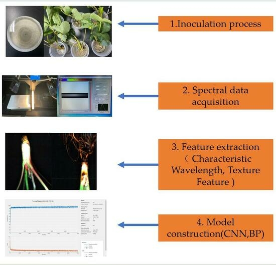
2.1. Strawberry Plants and Isolates

The samples of strawberry plants used were Fragaria × ananassa ‘Benihoppe’, cultivated by substrate plug cutting at the Lishui District Experimental Base, Nanjing, China. The tested strains of C. gloeosporioides were provided by the College of Plant Protection of Nanjing Agricultural University.

2.2. Inoculation of Strawberry Anthracnose Pathogen

After one year of storage at 4 °C, C. gloeosporioides isolate was retrieved from long-term storage and transferred twice on fresh potato dextrose agar (PDA) at 26 °C before inoculation. Inoculation was performed on the strawberry crown site during water cultivation of ‘Benihoppe’, a strawberry cultivar susceptible to C. gloeosporioides. For this experiment, fully expanded plants excised from strawberry plants grown in the field for ~4 weeks were placed into 20 mL of sterile water in a 6 cm paper cup. The C. gloeosporioides isolate was grown on PDA plates in a 9 cm Petri dish at 26 °C for 7 days (Figure 1a). Mycelia plugs (5 mm in diameter) were taken from the margin of each colony and inoculated on the same side of the crown with sterilized pipette tips (10 mm in diameter) to fix the peripheral mycelium plugs (Figure 1b). We fixed them with a pin, as shown in Figure 1c. The inoculated plants were arranged in a randomized complete block design and maintained at 26 °C and 95% humidity in light and dark for 12 h alternately. A total of 120 healthy strawberry seedlings of similar age, size, and growth were selected, of which 60 were inoculated with C. gloeosporioides and the other 60 served as the healthy control group. After small lesions were generated at the crown of the strawberries, spectral data collection was carried out.

In order to ensure the success of vaccination and ensure that the disease was caused by C. gloeosporioides, Koch’s rule was used for experimental verification [33]. Anthracnose pathogens were isolated from anthracnose foci inoculated tissue, as shown in Figure 2a,b. During the separation process, the surface was disinfected with 75% ethanol, soaked with 2% sodium hypochlorite for 60 s, and then soaked with 75% alcohol for 30 s. The surface was then washed with sterilized water three times. After drying, the infected site was transferred to the PDA containing ampicillin (an antibiotic to inhibit the growth of impurities) and cultured at 25 °C until fungal mycelium emerged from the necrotic tissue. After 5–7 days, the mycelium was transferred from the colony edge to the PDA. The isolated bacteria were inoculated on healthy plants (Figure 2c) and incidence was observed (Figure 2d). The content of Figure 2a is consistent with the observation of incidence in Figure 2d. Koch’s rule was validated, proving that the lesions at the inoculation site were indeed caused by C. gloeosporioides.

2.3. Hyperspectral Data Acquisition and Processing

The hyperspectral system is shown in Figure 3. The push-scan hyperspectral imaging system (Model HIS-VNIR-0001, Shanghai Wuling Optoelectronics Technology Co., Ltd, Shanghai, China) consisted of a spectral camera (Raptor EM285 high-sensitivity camera, Shanghai, China), a light source (21 V/200 W stable output halogen light source), a double-branch linear light tube (linear luminous length 15.24 cm), a dark box, a computer, an electronically controlled shift stage (IRCP0076, Isuzuoptics, Taiwan, China), and other components. The spectral wavelength range was 373–1033 nm, and the equipment parameters were adjusted for photographic accuracy, with a 35 mm imaging lens, an object distance of 27 cm, an exposure time of 2.0 ms, and a light intensity of 100 lx.

To convert the light intensity values into reflectance, the hyperspectral imaging system must be black-and-white calibrated before hyperspectral image acquisition trials of strawberry seedlings. The black-and-white calibration process commences with the acquisition of an image $I_w\left(i\right)$ using a standard white calibration plate, followed by the acquisition of an all-black calibrated image $I_d\left(i\right)$ with the lens cap on; finally, the calibration process is completed according to Equation (1) [34] using the following formula:

$$R\left(i\right)=\frac{I_r\left(i\right)-I_d\left(i\right)}{I_w\left(i\right)-I_d\left(i\right)}$$

(1)

where $R\left(i\right)$ is the relative of the rectification image, $I_r\left(i\right)$ is the original image reflectance of the experimental spectrum, $I_w\left(i\right)$ is the spectral reflectance after whiteboard correction, and $I_d\left(i\right)$ is the spectral reflectance after blackboard correction.

2.4. Methods for Constructing Hyperspectral Models

Figure 4 shows a flowchart of the diagnosis of strawberry anthracnose using different features of hyperspectral images and their combinations. There are three important steps: (i) the processing and analysis of hyperspectral data was performed based on spectral features and texture features; the feature wavelength was extracted using the SPA, CARS, and IRF. (ii) At the same time, GLCM was used to extract 12 dimensional TFs from the first three MNF images. (iii) Finally, spectral and texture features and their combinations were used to construct BP and CNN models, and the confusion matrices and modeling times were used to comprehensively evaluate the performance of different models.

2.4.1. Spectral Data Extraction

Raw files were imported using ENVI 5.3 software. A total of 120 healthy strawberry sample images and 120 diseased strawberry sample images were collected using hyperspectral instruments. The original collected hyperspectral data contain 306 wavelengths of information per image, and as the raw hyperspectral data contained a large amount of noise and invalid information at the beginning and end [35], 241 wavelengths from 447 nm to 965 nm were selected for data analysis to improve the accuracy of the later modeling [36]. Strawberry anthracnose has an incubation period during the onset period and will not immediately appear. To achieve the identification of asymptomatic infection status in the infected crown, hyperspectral data from the non-diseased area of the infected crown close to the lesion were extracted as an asymptomatic infection sample for analysis. The samples were divided into three categories according to the degree of infection: healthy samples, asymptomatic infections (invisible to the naked eye), and symptomatic infections (visible to the naked eye). A 5 × 5 region of interest (ROI) was selected in each of the healthy (H), asymptomatic infection (AI) and symptomatic infection (SI) data regions and the average spectral reflectance within the ROI was used as the spectral information. In total, 800 ROIs were extracted from each of the three classes of samples for a total of 2400 ROIs, and all data sets were subsequently preprocessed using Savitzky–Golay smoothing (SG) [37], while labels 1, 2, and 3 were used to represent healthy, asymptomatic infection, and symptomatic infection samples, respectively.

2.4.2. Characteristic Wavelength Selection

The SPA is a forward variable selection algorithm that minimizes vector space covariance. The specific steps of this algorithm are as follows [38]: first, select a spectral column vector in the spectral data as the starting vector and then calculate the projection of other column vectors on the starting vector. Next, select the smallest projection as the starting vector for the next projection until the number of selected variables reaches the number of input epochs. Finally, perform multiple linear regression on the extracted wavelength combinations; the combination of wavelengths with the highest prediction accuracy is selected as the optimal characteristic wavelength combination based on the local minimum root mean square error (RMSE).

The CARS is a feature variable selection method that combines Monte Carlo sampling with PLS model regression coefficients, mimicking the principle of survival of the fittest in Darwin’s theory [39]. In the CARS algorithm, adaptive reweighted sampling (ARS) retains the PLS model each time. The wavelengths in the subset with the smallest root mean square error of cross-validation (RMSECV) of the PLS model are selected as the characteristic wavelengths after several calculations.

The IRF algorithm is a random-frog-based wavelength interval selection method used to obtain all possible continuous intervals [40]; the spectrum is first divided into intervals by moving a window of fixed width across the spectrum. These overlapping intervals are ranked by applying random frogs and PLS, and the optimal combination of characteristic wavelengths is selected.

2.4.3. MFN Transform and Extraction of Texture Features

This study used ENVI5.3 remote sensing software for TF extraction. The generation of a large amount of redundant information in hyperspectral raw images is detrimental to model accuracy. The MNF separates the noise in the data and reduces the computational requirements for subsequent processing [41]. The first three MNF images (with a cumulative signal-to-noise ratio greater than 90%) were used to calculate and extract texture feature data. Finally, GLCM was used to extract texture features from the ROI of the first three MFN images.

2.4.4. Classification Recognition Model Construction

In this experiment, a machine learning BP neural network and deep learning CNN were chosen to construct a strawberry anthracnose recognition model using different features, including the SPA, CARS, IRF, TF, and their combinations. The BP neural network consists of an input layer, an implicit layer, and an output layer. Each layer consists of several nodes, and the layers are directly connected by weights. The core step is the gradient descent method, which uses a gradient search technique to minimize the mean squared error between the actual and desired outputs of the network. After several iterations of learning and training, the network parameters (weights and queue values) corresponding to the minimum error are determined and the training is completed [42].

The CNN is a feed-forward neural network with a convolutional structure. The convolutional structure can reduce the amount of memory occupied by the deep network; three key features—local perceptual field, weight sharing, and pooling layer—effectively reduce the number of parameters of the network. The CNN constructed in this paper is a one-dimensional convolutional neural network (1D-CNN) that uses spectral features and TFs as input layers to perform the classification [43].

2.4.5. Model Assessment

For model evaluation, classification accuracy, precision, recall, F1 score, and model building time calculated from the confusion matrix of the test set were used [44]. This is an example of a dichotomous classification problem. Accuracy represents the ratio of the number of correct predictions by the model to the number of all predictions. Precision represents the proportion of all outcomes predicted by the model as I (I = 1, 2, 3) that the model predicts correctly. Recall represents the proportion of model prediction pairs among all outcomes with the true value I (I = 1, 2, 3). The F1 score is the ratio of the product of the two-fold accuracy rate and the recall rate to the sum of the accuracy rate and the recall rate:

$$\mathrm{A}\mathrm{c}\mathrm{c}\mathrm{u}\mathrm{r}\mathrm{a}\mathrm{c}\mathrm{y}=\frac{TP+TN}{TP+FP+FN+TN}$$

(2)

$$\mathrm{P}\mathrm{r}\mathrm{e}\mathrm{c}\mathrm{i}\mathrm{s}\mathrm{i}\mathrm{o}\mathrm{n}=\frac{TP}{TP+FP}$$

(3)

$$\mathrm{R}\mathrm{e}\mathrm{c}\mathrm{a}\mathrm{l}\mathrm{l}=\frac{TP}{TP+FN}$$

(4)

$$\mathrm{F}1=\frac{2\times \mathrm{A}\mathrm{c}\mathrm{c}\mathrm{u}\mathrm{r}\mathrm{a}\mathrm{c}\mathrm{y}\times \mathrm{R}\mathrm{e}\mathrm{c}\mathrm{a}\mathrm{l}\mathrm{l}}{\mathrm{A}\mathrm{c}\mathrm{c}\mathrm{u}\mathrm{r}\mathrm{a}\mathrm{c}\mathrm{y}+\mathrm{R}\mathrm{e}\mathrm{c}\mathrm{a}\mathrm{l}\mathrm{l}}$$

(5)

where $TP$ means that the true value is positive and the predicted value is positive, which is a true positive example, $FP$ means that the value is negative and the predicted value is positive, which is a false positive example, $FN$ means that the true value is positive and the predicted value is negative, which is a false negative example, and $TN$ means that the true value is negative, and the predicted value is negative, which is a true negative example.

3. Results

3.1. Changes in Reflectance Caused by Anthracnose

Longitudinal macro diagrams of the inoculation of bacteria on the crown and healthy plants are shown in Figure 5. It can be seen that after the infected crown of strawberry anthracnose was cut, the crown turned dark brown from outside to inside and the infection site of anthracnose developed unilaterally or variably from outside to inside, while longitudinal cuts of healthy plants did not appear to blacken.

On the average spectral curve of all healthy, asymptomatic infected, and symptomatic infected samples obtained (Figure 6), the green line represents healthy samples, the blue line represents asymptomatic infected samples, and the red line represents symptomatic infected samples. It can be seen that the curve trend of healthy samples is significantly different from that of the infected samples.

The curve trend of healthy samples is 530–550 nm. There are obvious wave peaks between 580–620 nm and 656–700 nm, but no obvious wave peaks can be seen in the infected bacteria samples. Although the curves of asymptomatic infection and symptomatic infection samples have similar trends, it can be observed that as the disease deepens, anthracnose infection changes from asymptomatic infection to symptomatic infection, and the spectral reflectance also gradually declines. Looking at the sections of the three types of samples, it can be seen that the microscopic section of the symptomatic infected sample has a large number of spores, the microscopic section of the asymptomatic infected sample has a small number of spores, and the microscopic section of the healthy sample has no spores. Anthracnose infection has a certain latency: the initial infection state of strawberry anthracnose is black and brown, which then spreads from the infection point to the outside. After infection, the plant phenotype does not immediately show the corresponding symptoms, but the spectral reflectance can show this slight difference. The spectral changes in the disease development process are based on changes in plant pigment [45], water [46], and nutrient content [47], resulting in the above infection symptoms. These differences form the basis for the diagnosis of strawberry anthracnose.

3.2. Characteristic Wavelength Extraction Results and Analysis

The SPA, CARS, and IRF algorithms were used in the experiments to reduce the dimensionality of the dataset, while the SPA extracted characteristic wavelengths from full-spectrum data. The maximum selected wavelength parameter is set to 10, and the screening process for the SPA is shown in Figure A1 and Figure A2, including the trend of the root mean square error and the distribution of the characteristic wavelengths. As can be seen from Figure A1, the RMSE index is 0.425 when the combination of characteristic wavelengths is 5, and the corresponding wavelength is the characteristic wavelength. The distribution of the characteristic wavelengths is shown in Figure A2, in which the red circled parts are the filtered characteristic wavelengths.

The process of extracting characteristic wavelengths using the CARS algorithm is shown in Figure A3. The number of Monte Carlo samples was set to 100. The horizontal coordinate is the number of Monte Carlo sampling epochs, and the vertical coordinate includes the number of sampled variables (NSVs), the root mean square error of cross-validation (RMSECV), and the regression coefficients (RCs) with the number of Monte Carlo sampling epochs. The position of the red vertical line in Figure A3c shows that the RMSECV value is smallest when the number of samples is 40, which indicates that irrelevant information for anthracnose detection has been removed, and the RMSECV gradually increases after 40 samples. Therefore, the variables obtained from the 40th sampling were selected as 36 characteristic wavelengths.

The randomness of CARS sampling can lead to unstable modeling results. Three experiments on the extraction of characteristic wavelengths using CARS were carried out, and the parameters were set uniformly. The three extracted characteristic wavelengths were compared, and if three of them were extracted to the same band at the same time, they were retained as the final selection of the characteristic wavelength combination. The final 14 wavelengths (561, 564, 566, 583, 585, 591, 600, 602, 628, 647, 719, 749, 751, and 857 nm) were obtained according to this method.

The final characteristic wavelengths are shown in Figure 7d. Conducting multiple rounds of sampling to take repeated wavelengths reduces the randomness of sampling to meet the requirement of stability.

The characteristic wavelength was extracted by IRF algorithm. IRF selects the characteristic wavelength according to the selection likelihood of different wavelengths, and sets the random frog loop epoch parameter to 200. We set the selected probability to 100%. The extraction results are shown in Figure 8. Most of the sensitive wavelengths in Figure 8 are concentrated around 600–650 nm, 750–800 nm, and 900–920 nm. Finally, 566, 602, 604, 630, 767, 769, 804, 806, 905, 923 and 927 nm were selected. The locations circled in red in Figure 8 show these 11 characteristic wavelengths.

In summary, this experiment used SPA, CARS, and IRF to extract characteristic wavelengths. The characteristic wavelengths extracted by the three algorithms are shown in

Table 1. Characteristic wavelengths selected by SPA, CARS, and IRF.

Algorithm	Number of Characteristic Wavelengths	Characteristic Wavelengths (nm)
SPA	5	945, 901, 927, 591, 833
CARS	14	561, 564, 566, 583, 585, 591, 600, 602, 628, 647, 719, 749, 751, 857
IRF	11	566, 602, 604, 630, 767, 769, 804, 806, 905, 923, 927

. Compared with the full band, the number of wavelengths is greatly reduced, and these will be used as the spectral feature in input datasets for modeling and analysis in the future.

3.3. Texture Feature Extraction Results and Analysis

The TFs of strawberry images are of great importance in the diagnosis of anthracnose infection. Therefore, GLCM extracted four TFs (mean, homogeneity, entropy, correlation) from the previous three MNF images to generate a 12-dimension TF variable dataset. Figure 9 shows a boxplot of four features after normalization of the data. In the boxplot (with red circles indicating the mean and black lines indicating the median), the mean of the healthy sample is the smallest, and as the infection deepens, the mean gradually increases, with an increasing trend in the median. In terms of homogeneity means, the homogeneity mean of the healthy sample is the largest, and as the infection deepens, homogeneity gradually decreases, with a decreasing trend in the median. In terms of average information entropy, the average information entropy of health samples is the smallest. As the infection worsens, the mean information entropy increases progressively, and the median also shows an increasing trend. In terms of average correlation, the average correlation of healthy samples is the smallest. As infection deepens, the average correlation gradually increases, and the median also shows an increasing trend. The four texture elements vary sufficiently to show changes in different infection scenarios, but their range of variation is minimal, and their modeling effect could be modified in the future. Using the extracted characteristic wavelengths and TFs as input variables, the training and testing sets were divided into 3:1 samples, with 1800 training sets and 600 testing sets.

3.4. Recognition Results and Evaluation Based on Different Modeling Methods

The parameters of this BP model were set at the maximum number of 500 epochs, with a learning rate of 0.01, target training error of 1 × ${10}^{-6}$, and network structure of X-6-3 (X nodes in the input layer, 6 nodes in the hidden layer, and 3 nodes in the output layer). The identification results for each model are shown in

Table 2. BP neural network classification results.

Feature	Number of Feature Selection	Accuracy Rate (%)		Time (s)
		Train Set	Test Set
SPA	5	92.83	92.50	5.4
CARS	14	93.22	93.17	8.1
IRF	11	94.83	94.67	7.0
TF	12	75.33	75.50	7.2
SPA + TF	17	96.56	93.67	10.1
CARS + TF	26	95.17	93.50	11.4
IRF + TF	23	96.17	95.83	10.9

. Using the modeling of spectral features achieved over 90% accuracy for both the training and test sets, while the modeling of TFs only achieved 75% accuracy for both the training and test sets, making the spectral features more accurate in predicting disease from a feature perspective. Comparing the results of the fused data with those of the single-feature data, the fused-data modeling results were more accurate, and the accuracy was higher than that of the single spectral feature or texture feature modeling, in which the IRF + TF data fusion modeling effect was the most significant; the accuracy of the training set was 96.17% and that of the test set was 95.83%. To evaluate the model more effectively, the concepts of confusion matrix classification secondary metric precision (P), recall (R), and tertiary metric F1 score (F1 represents a range of combined accuracy and recall values between 0 and 1, the closer to 1 the better) were introduced. Figure 10a–g represents the confusion matrices of different model test sets. In the separate subgraph, the green areas represent consistency between the actual sample label and the predicted sample label, indicating that the classification result is correct. The red areas represent the difference between the actual sample labels and the predicted sample labels when the classification result is incorrect. The bottom row at the bottom of the graph is the recall rate, the last column is the precision rate, and the bottom right cell is the overall precision.

Based on the above findings, we can conclude that the modeling scheme with combined features is superior to that with a single feature. As can be seen from the results of the combined feature test sets in Figure 10 and Table 2, The results of IRF+TF+BP test set were 95.83%, SPA+TF+BP test set was 93.67%, and CARS+TF+BP test set was 93.50%. The modeling scheme combining IRF and TF had the highest diagnostic efficiency for anthracnose disease.

The parameters of this CNN model were set using the Adam gradient descending algorithm. After the maximum of 500 training repetitions, the initial learning rate was 0.001; after 450 training repetitions, a learning rate of 0.001 × 0.5 after each training repetition was found to disrupt the data set. The recognition results for each CNN model are shown in

Table 3. CNN (convolutional neural network) classification results.

Feature	Number of Feature Selection	Accuracy Rate (%)		Time (s)
		Train Set	Test Set
SPA	5	94.78	94.50	95
CARS	14	95.61	93.83	101
IRF	11	95.61	94.50	97
TF	12	90	79.50	99
SPA + TF	17	100	95.33	110
CARS + TF	26	100	95.83	118
IRF + TF	23	100	95.50	114

. The test set results for SPA + CNN, CARS + CNN, and IRF + CNN based on spectral characteristics were 94.5%, 93.83%, and 94.5%, respectively. The result for the TFs-based test set TF + CNN was 79.5%. In Table 2, the results for SPA + BP, CARS + BP, and IRF + BP test sets are shown, which were 92.5%, 93.17%, and 94.67%, respectively. The TF + BP of the test set based on TFs was 75.5%. Compared with the above two modeling results, except for the IRF + CNN and IRF + BP test sets, the results of the other CNN test sets were significantly better than the BP test sets, which proves that CNN is superior to BP from the perspective of accuracy.

The most important goal was to explore the recognition of asymptomatic infection of strawberry anthracnose via data fusion and deep learning.

Table 4. Classification effect of BP neural network and CNN model test set.

Model	Time/s	P/%			R/%			F1
		H	AI	SI	H	AI	SI	H	AI	SI
SPA + BP	5.4	99.00	90.50	88.50	99.50	87.40	91.10	0.9925	0.8892	0.8978
CARS + BP	8.1	100.00	86.60	93.50	100.00	93.30	86.90	1.0000	0.8983	0.9008
IRF + BP	7	100.00	90.00	93.40	100.00	93.80	89.50	1.0000	0.9186	0.9141
TF + BP	7.2	72.30	75.00	80.10	84.80	67.50	74.70	0.7805	0.7105	0.7731
SPA + TF + BP	10.1	100.00	90.50	90.30	99.50	91.40	89.80	0.9975	0.9095	0.9005
CARS + TF + BP	11.4	99.50	90.90	90.70	99.50	91.30	90.20	0.9950	0.9110	0.9045
IRF + TF + BP	10.9	99.10	93.50	94.50	100.00	94.00	93.00	0.9955	0.9375	0.9374
SPA + CNN	95	99.00	89.80	94.80	100.00	93.20	90.90	0.9950	0.9147	0.9281
CARS + CNN	101	100.00	90.70	91.00	100.00	91.10	90.50	1.0000	0.9090	0.9075
IRF + CNN	97	100.00	89.60	93.80	100.00	94.50	88.40	1.0000	0.9198	0.9102
TF + CNN	99	78.90	76.80	82.40	80.50	69.80	88.30	0.7969	0.7313	0.8525
SPA + TF + CNN	110	96.50	93.90	95.60	99.00	92.50	94.60	0.9773	0.9319	0.9510
CARS + TF + CNN	118	98.50	93.10	95.90	99.50	94.50	93.50	0.9900	0.9380	0.9468
IRF + TF + CNN	114	98.00	96.50	92.10	99.00	91.10	96.90	0.9850	0.9372	0.9444

and Figure 11 show the identification of asymptomatic strawberry anthracnose; the F1 scores of SPA + TF + BP, CARS + TF + BP, and IRF + TF + BP for the recognition of asymptomatic strawberry anthracnose were 0.9095, 0.911, and 0.9375, respectively, while for SPA + TF + CNN, CARS + TF + CNN, and IRF + TF + CNN, the F1 scores corresponded to 0.9319, 0.938, and 0.9372. Compared with the F1 score, the combined features and CNN were more accurate in diagnosing asymptomatic infection samples. The experimental results demonstrate that data fusion combined with deep learning is feasible and effective for identifying asymptomatic strawberry anthracnose infection.

4. Discussion

Previous studies only identified isolated strawberry leaf anthracnose or gray mold infection [29,48], and did not carry out in-depth studies on the asymptomatic infection stage of live plants. Anthracnose infection of strawberry leaves does not cause the death of the whole plant, while anthracnose infection of the crown results in a high probability of strawberry plant death. In this study, we demonstrated the feasibility of using spectral features and TFs and combinations thereof to diagnose asymptomatic infections of strawberry anthracnose. In this experiment, the characteristic wavelength extraction algorithms SPA, CARS, and IRF were used to extract 5, 14, and 11 characteristic wavelengths, respectively, from the original 241-wavelength dataset. The classification and distinguishing model of strawberry anthracnose was established according to the combination of characteristic wavelengths. Previous studies have achieved good results in using extracted characteristic wavelength algorithms to detect plant physiological indicators and diseases [49,50,51]. After obtaining raw hyperspectral data, feature extraction is crucial. The raw data volume of the captured hyperspectral images is large (up to 2–3 G per image), and has the typical characteristics of high data volume. Furthermore, hyperspectral images have a high spectral resolution and contain a large number of wavelengths, resulting in high feature dimensionality. In addition, hyperspectral images have a strong correlation between various wavelengths, and the interspectral correlation coefficients of the images are large, which can easily cause redundant hyperspectral information stacking. It is necessary to solve the problems of data correlation, redundancy, and covariance brought about by large numbers of hyperspectral data and large data volume to reduce the complexity of the model and improve the modeling accuracy and operation speed. Using the characteristic wavelength extraction algorithm can significantly improve the accuracy and speed of the model. As shown in Table 2 and Table 3, the accuracy rates of SPA + BP and SPA + CNN test sets were observed to be 92.5% and 94.5%, respectively; the accuracy rates of CARS + BP and CARS + CNN test sets were 93.17% and 93.83%, respectively; and the accuracy rates of IRF + BP and IRF + CNN test sets were 94.67% and 94.5%, respectively. In terms of data compression, compared to IRF and CARS, the SPA extracted the least feature wavelengths. In terms of modeling effectiveness, IRF extracted more effective characteristic wavelengths and had the highest modeling accuracy.

Infection of the strawberry crown by C. gloeosporioides will not only cause a change in spectral reflectance but also will cause a structural change in the crown surface. In the area of hyperspectral images for distinguishing model plant disease, there is less research on disease recognition using image features, and results have not been meaningful [52]. In addition, for most of the hyperspectral images, principal component analysis (PCA) is used to reduce the dimensions, and the later modeling effect is poor [13]. MNF is essentially a two-layered principal component transformation, and MNF transformation is similar to PCA transformation in that it is an orthogonal transformation in which the elements in the transformed vector are uncorrelated with each other. The first component gathers a large amount of information, and as the dimension increases, the image quality decreases. Data are arranged in descending order of signal-to-noise ratio, unlike PCA changes in descending order of variance, thus overcoming the impact of noise on image quality. Because the noise in the transformation process has unit variance and is not correlated between bands, it is superior to PCA transformation. This experiment used MNF dimensionality reduction to extract 12 dimensional image texture features from hyperspectral images and construct a recognition model for strawberry anthracnose. The accuracy of the TF + BP test set was 75.5%, and the accuracy of the TF + CNN test set was 79.5%, so the model was constructed using the CNN. The BP neural network and TF showed good performance, which proved the feasibility of diagnosing strawberry anthracnose by the TF of hyperspectral images. In addition to the mean, homogeneity, entropy, and correlation used in this experiment, the image TFs also have variance, contrast, difference, and angular second moment. These other texture features can be used for modeling and analysis in future research experiments.

We used spectral and texture features combined with different modeling methods to identify infected strawberry anthracnose and explore the improvement in data fusion on model accuracy. This study separately observed the comparison of the accuracy of spectral and TF modeling in Table 2 and Table 3. It can be seen that the accuracy of the spectral feature modeling test set has reached over 90%, while the accuracy of the TF modeling test set has not exceeded 80%. Spectral features are more sensitive than TFs, and the modeling effect is more significant. Due to the small differences between asymptomatic infections and health data images, the TFs cause the model to be unstable and recognition accuracy is poor, but they can be used as fusion features to improve the accuracy of the model in the future. Table 2 and Table 3 show the results of two-feature fusion data and single-feature data modeling. The accuracy of the spectral feature modeling test set was about 92–93% and the accuracy of the TF test set was 75–79.5%, while the accuracy of fusion data test set steadily improved to 93–95%, proving that fusion data modeling is more accurate in distinguishing and modeling than using spectral features or TFs alone.

Different modeling methods were used to distinguish the asymptomatic infection state of strawberry anthracnose and to explore the improvement in the accuracy of deep learning CNN. Previous studies mostly used a single machine learning method with a small sample size for modeling and analysis [22,23,24,25,26,27]. Khairunniza-Beio et al. only used SVM for modeling without considering deep learning modeling [49], while the present experiment used thousands of sample sizes for the training of a deep learning model. Table 2 and Table 3 show that the recognition rate of combined features and BP modeling was 93–95%, and the recognition rate of combined features and the CNN modeling test set is stable at about 95%. Table 4 shows that the F1 score distinctions between combined features and BP modeling for asymptomatic infection were 0.9095, 0.911, and 0.9375, respectively. For asymptomatic infection, the differences in F1 scores between combined features and CNN modeling was 0.9319, 0.938, and 0.9372, respectively, and F1 was stable at 0.93. The CNN is more stable than the traditional machine learning BP neural network when considering only the robustness of model recognition and the accuracy of asymptomatic infection recognition, without considering other modeling factors.

This experiment considered the development and application of the sensor in the later stage. The time and recognition accuracy required for BP neural network modeling and CNN modeling were compared. It can be observed from Table 4 that the modeling time of BP neural networks was between 5.4 and −11.4 s, while that of CNN was between 95 and −118 s. The modeling time is affected by the volume of input data and the number of layers of the model; the CNN modeling process is relatively complex due to the multiple layers and large amount of computational data. By comprehensively comparing the accuracy and time of the 14 models, the IRF + TF + BP model test set had accuracies of 99.1%, 93.5%, and 94.5%, respectively, for healthy, asymptomatic, and symptomatic samples at all levels, with recall rates of 100%, 94%, 93% and F1 scores of 0.9955, 0.9375, and 0.9374, respectively. A modeling time of 10.9 s was the best comprehensive performance demonstrated by any model. The above results provide technical support for the detection of the asymptomatic infection of strawberry anthracnose and provide a reference for the development of ultra-low-altitude remote sensing disease monitoring using plant protection drones and handheld equipment for strawberry anthracnose.

5. Conclusions

This study explored the possibility of combining hyperspectral technology with machine learning and deep learning in the identification of asymptomatic infection of strawberry anthracnose. The crown region of strawberry plants was used as the research object, and a hyperspectral dataset of 447–965 nm was collected. Five characteristic wavelengths were extracted using the SPA: 945, 901, 927, 591, and 833 nm. CARS was used to extract 14 characteristic wavelengths: 561, 564, 566, 583, 585, 591, 600, 602, 628, 647, 719, 749, 751, and 857 nm. IRF was used to extract 11 characteristic wavelengths: 566, 602, 604, 630, 767, 769, 804, 806, 905, 923, and 927 nm. We extracted 12 dimensional TFs from the first three MNF images using GLCM, and a BP neural network and CNN were established for modeling and analysis using spectral features, TFs, and fused data as input variables. The IRF + TF + BP model test set has accuracy of 99.1%, 93.5%, and 94.5%, respectively, for healthy, asymptomatic, and symptomatic samples at all levels, with recall rates of 100%, 94%, and 93% and F1 scores of 0.9955, 0.9375, and 0.9374. The modeling time of 10.9 s was the best comprehensive performance demonstrated by any model.

References

1. Ji, Y.; Li, X.; Gao, Q.; Geng, C.; Duan, K. Colletotrichum species pathogenic to strawberry: Discovery history, global diversity, prevalence in China, and the host range of top two species. Phytopathol. Res. 2022, 4, 42. [Google Scholar] [CrossRef]
2. Chen, X.Y.; Dai, D.J.; Zhao, S.F.; Shen, Y.; Wang, H.D.; Zhang, C.Q. Genetic diversity of Colletotrichum spp. causing strawberry anthracnose in Zhejiang, China. Plant Dis. 2020, 104, 1351–1357. [Google Scholar] [CrossRef] [PubMed]
3. Jian, Y.; Li, Y.; Tang, G.; Zheng, X.; Khaskheli, M.I.; Gong, G. Identification of Colletotrichum species associated with anthracnose disease of strawberry in Sichuan province, China. Plant Dis. 2021, 105, 3025–3036. [Google Scholar] [CrossRef] [PubMed]
4. Soares, V.F.; Velho, A.C.; Carachenski, A.; Astolfi, P.; Stadnik, M.J. First report of Colletotrichum karstii causing anthracnose on strawberry in Brazil. Plant Dis. 2021, 105, 3295. [Google Scholar] [CrossRef] [PubMed]
5. Smith, B.J. Epidemiology and pathology of strawberry anthracnose: A North American perspective. HortScience 2008, 43, 69–73. [Google Scholar] [CrossRef]
6. Yang, J.; Duan, K.; Liu, Y.; Song, L.; Gao, Q.H. Method to detect and quantify colonization of anthracnose causal agent Colletotrichum gloeosporioides species complex in strawberry by real-time PCR. J. Phytopathol. 2022, 170, 326–336. [Google Scholar] [CrossRef]
7. Shengfan, H.; Junjie, L.; Tengfei, X.; Xuefeng, L.; Xiaofeng, L.; Su, L.; Hongqing, W. Simultaneous detection of three crown rot pathogens in field-grown strawberry plants using a multiplex PCR assay. Crop Prot. 2022, 156, 105957. [Google Scholar] [CrossRef]
8. Miftakhurohmah; Mutaqin, K.H.; Soekarno, B.P.W.; Wahyuno, D.; Hidayat, S.H. Identification of endogenous and episomal piper yellow mottle virus from the leaves and berries of black pepper (Piper nigrum). Austral. Plant Pathol. 2021, 50, 431–434. [Google Scholar] [CrossRef]
9. Schoelz, J.; Volenberg, D.; Adhab, M.; Fang, Z.; Klassen, V.; Spinka, C.; Rwahnih, M.A. A survey of viruses found in grapevine cultivars grown in Missouri. Am. J. Enol. Vitic. 2021, 72, 73–84. [Google Scholar] [CrossRef]
10. Khudhair, M.; Obanor, F.; Kazan, K.; Gardiner, D.M.; Aitken, E.; McKay, A.; Giblot-Ducray, D.; Simpfendorfer, S.; Thatcher, L.F. Genetic diversity of Australian Fusarium pseudograminearum populations causing crown rot in wheat. Eur. J. Plant Pathol. 2021, 159, 741–753. [Google Scholar] [CrossRef]
11. Lowe, A.; Harrison, N.; French, A.P. Hyperspectral image analysis techniques for the detection and classification of the early onset of plant disease and stress. Plant Methods 2017, 13, 80. [Google Scholar] [CrossRef] [PubMed]
12. Zhang, N.; Yang, G.; Pan, Y.; Yang, X.; Chen, L.; Zhao, C. A review of advanced technologies and development for Hyperspectral-based plant disease detection in the past three decades. Remote Sens. 2020, 12, 3188. [Google Scholar] [CrossRef]
13. Terentev, A.; Dolzhenko, V.; Fedotov, A.; Eremenko, D. Current state of hyperspectral remote sensing for early plant disease detection: A review. Sensors 2022, 22, 757. [Google Scholar] [CrossRef]
14. Wu, W.; Zhang, Z.; Zheng, L.; Han, C.; Wang, X.; Xu, J.; Wang, X. Research progress on the early monitoring of pine wilt disease using hyperspectral techniques. Sensors 2020, 20, 3729. [Google Scholar] [CrossRef] [PubMed]
15. Che Ya, N.N.; Mohidem, N.A.; Roslin, N.A.; Saberioon, M.; Tarmidi, M.Z.; Arif Shah, J.; Fazlil Ilahi, W.F.; Man, N. Mobile computing for pest and disease management using spectral signature analysis: A review. Agronomy 2022, 12, 967. [Google Scholar] [CrossRef]
16. Yuan, L.; Yan, P.; Han, W.; Huang, Y.; Wang, B.; Zhang, J.; Zhang, H.; Bao, Z. Detection of anthracnose in tea plants based on hyperspectral imaging. Comput. Electron. Agric. 2019, 167, 105039. [Google Scholar] [CrossRef]
17. Appeltans, S.; Pieters, J.G.; Mouazen, A.M. Detection of leek white tip disease under field conditions using hyperspectral proximal sensing and supervised machine learning. Comput. Electron. Agric. 2021, 190, 106453. [Google Scholar] [CrossRef]
18. Pérez-Roncal, C.; Arazuri, S.; Lopez-Molina, C.; Jarén, C.; Santesteban, L.G.; López-Maestresalas, A. Exploring the potential of hyperspectral imaging to detect Esca disease complex in asymptomatic grapevine leaves. Comput. Electron. Agric. 2022, 196, 106863. [Google Scholar] [CrossRef]
19. Xuan, G.; Li, Q.; Shao, Y.; Shi, Y. Early diagnosis and pathogenesis monitoring of wheat powdery mildew caused by Blumeria graminis using hyperspectral imaging. Comput. Electron. Agric. 2022, 197, 106921. [Google Scholar] [CrossRef]
20. Xie, C.; Yang, C.; He, Y. Hyperspectral imaging for classification of healthy and gray mold diseased tomato leaves with different infection severities. Comput. Electron. Agric. 2017, 135, 154–162. [Google Scholar] [CrossRef]
21. Zhang, J.; Tian, Y.; Yan, L.; Wang, B.; Wang, L.; Xu, J.; Wu, K. Diagnosing the symptoms of sheath blight disease on rice stalk with an in-situ hyperspectral imaging technique. Biosyst. Eng. 2021, 209, 94–105. [Google Scholar] [CrossRef]
22. Fazari, A.; Pellicer-Valero, O.J.; Gómez-Sanchıs, J.; Bernardi, B.; Cubero, S.; Benalia, S.; Zimbalatti, G.; Blasco, J. Application of deep convolutional neural networks for the detection of anthracnose in olives using VIS/NIR hyperspectral images. Comput. Electron. Agric. 2021, 187, 106252. [Google Scholar] [CrossRef]
23. Gao, Z.; Khot, L.R.; Naidu, R.A.; Zhang, Q. Early detection of grapevine leafroll disease in a red-berried wine grape cultivar using hyperspectral imaging. Comput. Electron. Agric. 2020, 179, 105807. [Google Scholar] [CrossRef]
24. Conrad, A.O.; Li, W.; Lee, D.Y.; Wang, G.L.; Rodriguez-Saona, L.; Bonello, P. Machine Learning-based presymptomatic detection of rice sheath blight using -spectral profiles. Plant Phenomics 2020, 2020, 8954085. [Google Scholar] [CrossRef] [PubMed]
25. Jin, X.; Jie, L.; Wang, S.; Qi, H.; Li, S. Classifying wheat hyperspectral pixels of healthy heads and fusarium head blight disease using a deep neural network in the wild field. Remote Sens. 2018, 10, 395. [Google Scholar] [CrossRef]
26. Zhao, X.; Zhang, J.; Huang, Y.; Tian, Y.; Yuan, L. Detection and discrimination of disease and insect stress of tea plants using hyperspectral imaging combined with wavelet analysis. Comput. Electron. Agric. 2022, 193, 106717. [Google Scholar] [CrossRef]
27. Sha, W.; Hu, K.; Weng, S. Statistic and network features of RGB and hyperspectral Imaging for determination of black root mold infection in apples. Foods 2023, 12, 1608. [Google Scholar] [CrossRef] [PubMed]
28. Cen, Y.; Huang, Y.; Hu, S.; Zhang, L.; Zhang, J. Early detection of bacterial wilt in tomato with portable hyperspectral spectrometer. Remote Sens. 2022, 14, 2882. [Google Scholar] [CrossRef]
29. Jiang, Q.; Wu, G.; Tian, C.; Li, N.; Yang, H.; Bai, Y.; Zhang, B. Hyperspectral imaging for early identification of strawberry leaves diseases with machine learning and spectral fingerprint features. Infrared Phys. Technol. 2021, 118, 103898. [Google Scholar] [CrossRef]
30. Miller-Butler, M.A.; Smith, B.J.; Curry, K.J.; Blythe, E.K. Evaluation of detached strawberry leaves for anthracnose disease severity using image analysis and visual ratings. HortScience 2019, 54, 2111–2117. [Google Scholar] [CrossRef]
31. Genangeli, A.; Allasia, G.; Bindi, M.; Cantini, C.; Cavaliere, A.; Genesio, L.; Giannotta, G.; Miglietta, F.; Gioli, B. A novel hyperspectral method to detect moldy core in apple fruits. Sensors 2022, 22, 4479. [Google Scholar] [CrossRef] [PubMed]
32. Feng, S.; Zhao, D.; Guan, Q.; Li, J.; Liu, Z.; Jin, Z.; Li, G.; Xu, T. A deep convolutional neural network-based wavelength selection method for spectral characteristics of rice blast disease. Comput. Electron. Agric. 2022, 199, 107199. [Google Scholar] [CrossRef]
33. Wu, J.P.; Zhou, J.; Jiao, Z.B.; Fu, J.P.; Xiao, Y.; Guo, F.L. Amorphophallus konjac anthracnose caused by Colletotrichum siamense in China. J. Appl. Microbiol. 2020, 128, 225–231. [Google Scholar] [CrossRef] [PubMed]
34. Zhao, D.; Liu, S.; Yang, X.; Ma, Y.; Zhang, B.; Chu, W. Research on camouflage recognition in simulated operational environment based on hyperspectral imaging technology. J. Spectrosc. 2021, 2021, 6629661. [Google Scholar] [CrossRef]
35. Barreto, A.; Paulus, S.; Varrelmann, M.; Mahlein, A. Hyperspectral imaging of symptoms induced by Rhizoctonia solani in sugar beet: Comparison of input data and different machine learning algorithms. J. Plant Dis. Prot. 2020, 127, 441–451. [Google Scholar] [CrossRef]
36. Wei, X.; Johnson, M.A.; Langston, D.B.; Mehl, H.L.; Li, S. Identifying optimal wavelengths as disease signatures using hyperspectral sensor and machine learning. Remote Sens. 2021, 13, 2833. [Google Scholar] [CrossRef]
37. An, C.; Yan, X.; Lu, C.; Zhu, X. Effect of spectral pretreatment on qualitative identification of adulterated bovine colostrum by near-infrared spectroscopy. Infrared Phys. Technol. 2021, 118, 103869. [Google Scholar] [CrossRef]
38. Zhu, H.; Chu, B.; Zhang, C.; Liu, F.; Jiang, L.; He, Y. Hyperspectral imaging for presymptomatic detection of tobacco disease with successive projections algorithm and Machine-learning classifiers. Sci. Rep. 2017, 7, 4125. [Google Scholar] [CrossRef]
39. Liu, S.; Yu, H.; Sui, Y.; Zhou, H.; Zhang, J.; Kong, L.; Dang, J.; Zhang, L. Classification of soybean frogeye leaf spot disease using leaf hyperspectral reflectance. PLoS ONE 2021, 16, e257008. [Google Scholar] [CrossRef]
40. Liu, N.; Qiao, L.; Xing, Z.; Li, M.; Sun, H.; Zhang, J.; Zhang, Y. Detection of chlorophyll content in growth potato based on spectral variable analysis. Spectr. Lett. 2020, 53, 476–488. [Google Scholar] [CrossRef]
41. Zhang, B.; Li, J.; Fan, S.; Huang, W.; Zhao, C.; Liu, C.; Huang, D. Hyperspectral imaging combined with multivariate analysis and band math for detection of common defects on peaches (Prunus persica). Comput. Electron. Agric. 2015, 114, 14–24. [Google Scholar] [CrossRef]
42. Liu, L.; Dong, Y.; Huang, W.; Du, X.; Ma, H. Monitoring wheat fusarium head blight using unmanned aerial vehicle hyperspectral imagery. Remote Sens. 2020, 12, 3811. [Google Scholar] [CrossRef]
43. Zhang, J.; Yang, Y.; Feng, X.; Xu, H.; Chen, J.; He, Y. Identification of bacterial blight resistant rice seeds using terahertz imaging and hyperspectral imaging combined with convolutional neural network. Front. Plant Sci. 2020, 11, 821. [Google Scholar] [CrossRef] [PubMed]
44. Riefolo, C.; Antelmi, I.; Castrignanò, A.; Ruggieri, S.; Galeone, C.; Belmonte, A.; Muolo, M.R.; Ranieri, N.A.; Labarile, R.; Gadaleta, G.; et al. Assessment of the hyperspectral data analysis as a tool to diagnose Xylella fastidiosa in the asymptomatic leaves of olive plants. Plants 2021, 10, 683. [Google Scholar] [CrossRef] [PubMed]
45. Blackburn, G.A. Quantifying chlorophylls and caroteniods at leaf and canopy scales: An evaluation of some hyperspectral approaches. Remote Sens. Environ. 1998, 66, 273–285. [Google Scholar] [CrossRef]
46. Bruning, B.; Liu, H.; Brien, C.; Berger, B.; Lewis, M.; Garnett, T. The development of hyperspectral distribution maps to predict the content and distribution of nitrogen and water in wheat (Triticum aestivum). Front. Plant Sci. 2019, 10, 1380. [Google Scholar] [CrossRef] [PubMed]
47. Eshkabilov, S.; Lee, A.; Sun, X.; Lee, C.W.; Simsek, H. Hyperspectral imaging techniques for rapid detection of nutrient content of hydroponically grown lettuce cultivars. Comput. Electron. Agric. 2021, 181, 105968. [Google Scholar] [CrossRef]
48. Wu, G.; Fang, Y.; Jiang, Q.; Cui, M.; Li, N.; Ou, Y.; Diao, Z.; Zhang, B. Early identification of strawberry leaves disease utilizing hyperspectral imaging combing with spectral features, multiple vegetation indices and textural features. Comput. Electron. Agric. 2023, 204, 107553. [Google Scholar] [CrossRef]
49. Khairunniza-Bejo, S.; Shahibullah, M.S.; Azmi, A.N.N.; Jahari, M. Non-destructive detection of asymptomatic Ganoderma boninense infection of oil palm seedlings using NIR-hyperspectral data and support vector machine. Appl. Sci. 2021, 11, 10878. [Google Scholar] [CrossRef]
50. Pane, C.; Manganiello, G.; Nicastro, N.; Cardi, T.; Carotenuto, F. Powdery mildew caused by Erysiphe cruciferarum on wild rocket (Diplotaxis tenuifolia): Hyperspectral imaging and machine learning modeling for non-destructive disease detection. Agriculture 2021, 11, 337. [Google Scholar] [CrossRef]
51. Zhao, J.; Fang, Y.; Chu, G.; Yan, H.; Hu, L.; Huang, L. Identification of Leaf-scale wheat powdery mildew (Blumeria graminis f. sp. tritici) combining hyperspectral imaging and an SVM classifier. Plants 2020, 9, 936. [Google Scholar] [CrossRef]
52. Guo, A.; Huang, W.; Ye, H.; Dong, Y.; Ma, H.; Ren, Y.; Ruan, C. Identification of wheat yellow rust using spectral and texture features of hyperspectral images. Remote Sens. 2020, 12, 1419. [Google Scholar] [CrossRef]
Figure 1. Inoculation process. (a) Colony of C. gloeosporioides; (b) inoculation diagram; (c) enlarged view of the crown of the inoculated root.
Remotesensing 15 04640 g001
Figure 2. Koch’s postulate verification. (a) C. gloeosporioides inoculation crown longitudinal cut; (b) pathogen lesion site to be isolated; (c) inoculate healthy plant; (d) profile of the inoculation site.
Remotesensing 15 04640 g002
Figure 3. Hyperspectral image acquisition system.
Remotesensing 15 04640 g003
Figure 4. Data processing flow chart.
Remotesensing 15 04640 g004
Figure 5. Longitudinal comparison between inoculated and healthy strawberries. (a) Inoculated plants, (b) healthy plants.
Remotesensing 15 04640 g005
Figure 6. Average spectral curves for different samples compared using sectional microscopy. Note: Microscope observation magnification is 25×.
Remotesensing 15 04640 g006
Figure 7. CARS used to extract characteristic wavelength distribution.
Remotesensing 15 04640 g007
Figure 8. IRF algorithm extracts characteristic wavelengths.
Remotesensing 15 04640 g008
Figure 9. Healthy, asymptomatic, and symptomatic infection box diagram. (a) Mean, (b) homogeneity, (c) entropy, (d) correlation. Note: The red dots in the block diagram represent the mean of the data.
Remotesensing 15 04640 g009
Figure 10. Confusion matrices of BP neural network test set. (a) SPA + BP test set confusion matrix, (b) CARS + BP test set confusion matrix, (c) IRF + BP test set confusion matrix, (d) TF + BP test set confusion matrix, (e) SPA + TF + BP test set confusion matrix, (f) CARS + TF + BP test set confusion matrix, (g) IRF + TF + BP test set confusion matrix.
Remotesensing 15 04640 g010
Figure 11. CNN test set confusion matrices: (a) SPA + CNN test set confusion matrix, (b) CARS + CNN test set confusion matrix, (c) IRF + CNN test set confusion matrix, (d) TF + CNN test set confusion matrix, (e) SPA + TF + CNN test set confusion matrix, (f) CARS + TF + CNN test set confusion matrix, (g) IRF + TF + CNN test set confusion matrix.
Remotesensing 15 04640 g011aRemotesensing 15 04640 g011b