
Areca Yellow Leaf Disease Severity Monitoring Using UAV-Based Multispectral and Thermal Infrared Imagery

1
Key Laboratory of Biomedical Engineering of Hainan Province, School of Biomedical Engineering, Hainan University, Haikou 570228, China
2
Britton Chance Center for Biomedical Photonics, Wuhan National Laboratory for Optoelectronics, Huazhong University of Science and Technology, Wuhan 430074, China
3
MoE Key Laboratory for Biomedical Photonics, Huazhong University of Science and Technology, Wuhan 430074, China
*
Authors to whom correspondence should be addressed.
†
These authors contributed equally to this work.
Remote Sens. 2023, 15(12), 3114; https://doi.org/10.3390/rs15123114
Submission received: 21 April 2023
/
Revised: 8 June 2023
/
Accepted: 12 June 2023
/
Published: 14 June 2023
(This article belongs to the Special Issue Spectral Imaging Technology for Crop Disease Detection)
Abstract
:The areca nut is the primary economic source for some farmers in southeast Asia. However, the emergence of areca yellow leaf disease (YLD) has seriously reduced the annual production of areca nuts. There is an urgent need for an effective method to monitor the severity of areca yellow leaf disease (SAYD). This study selected an areca orchard with a high incidence of areca YLD as the study area. An unmanned aerial vehicle (UAV) was used to acquire multispectral and thermal infrared data from the experimental area. The ReliefF algorithm was selected as the feature selection algorithm and ten selected vegetation indices were used as the feature variables to build six machine-learning classification models. The experimental results showed that the combination of ReliefF and the Random Forest algorithm achieved the highest accuracy in the prediction of SAYD. Compared to manually annotated true values, the R2 value, root mean square error, and mean absolute percentage error reached 0.955, 0.049, and 1.958%, respectively. The Pearson correlation coefficient between SAYD and areca canopy temperature (CT) was 0.753 (p value < 0.001). The experimental region was partitioned, and a nonlinear fit was performed using CT versus SAYD. Cross-validation was performed on different regions, and the results showed that the R2 value between the predicted result of SAYD by the CT and actual value reached 0.723. This study proposes a high-precision SAYD prediction method and demonstrates the correlation between the CT and SAYD. The results and methods can also provide new research insights and technical tools for botanical researchers and areca practitioners, and have the potential to be extended to more plants.
1. Introduction
Areca (Areca catechu L.) is an evergreen tree of the genus areca in the palm family. It is an essential herbal medicine, mainly distributed in some countries in East Asia, South Asia, and Southeast Asia. It is an essential economic crop in Southeast Asian countries and is economically important to China and India [1]. Areca is also a popular traditional herbal medicine that can be chewed to disperse accumulated fluid in the abdominal cavity and kill worms; it can potentially treat parasitic diseases, digestive function disorders, and depression [2]. In addition, the extracts of areca strongly enhanced viability against H202-induced oxidative damage in Chinese hamster lung fibroblast cells [3]. Areca waste is also a promising adsorbent for wastewater treatment [4].
The areca yellow leaf disease (YLD) has now become the biggest constraint on the development of the areca industry. The occurrence of areca yellow leaf disease starts from the second to the last or third leaf, then spreads upwards, and the entire tree’s leaves become yellow. The flower spikes of areca trees wither, unable to bloom and bear fruit, or bear a small amount of inedible black fruits. Yellow leaf disease is a devastating disaster for areca, with a prevalence of up to a 90 and 78 to 80% yield reduction in severe parks. In the past, detecting the severity of areca yellow leaf disease (SAYD) mainly relied on manual observation [1], which required a lot of human and material resources. Nowadays, the development of remote sensing has provided a new method to monitor SAYD.
Unmanned aerial vehicles (UAVs) are increasingly used for monitoring plant diseases because of their convenience, simplicity, and cheapness. Different types of cameras can be mounted on them to form different observation systems [5]—for example, visible light, thermal infrared, and multispectral sensors. We can use UAVs with different sensors to measure and monitor the potential structural properties of forests [6], monitor beach litter [7], and build road detection and tracking frameworks [8]. Spectroscopic imaging provides a promising solution for large-scale disease monitoring under field conditions and is receiving ever-increasing research interest [9]. Pathogens cause a reduction of plant ChlorophyII content in the visible and red-edge region of the spectrum due to necrotic or chlorotic lesions [10]. UAVs equipped with multispectral sensors to obtain spectral bands and spectral vegetation indices with high resolution allow the development of an automated yellow rust detection system with good classification [11]. Those equipped with visible and near-infrared sensors are able to describe the relationship between late blight incidences and spectral variation in the potato [12]. Laboratory scans and hyperspectral-equipped UAVs have been jointly used to identify and classify bacterial tomato spot (BS), target spot (TS), and tomato yellow leaf curl (TYLC) through the machine learning approach; the method reached 98, 96, and 100% accuracy for BS, TS, and TYLC, respectively [13]. Vegetation indices and spectral differences between healthy and infected citrus trees have been compared using drone-based multispectral images. The experiments showed that UAV-based phenotypic information of citrus could be an essential indicator for distinguishing infected citrus [14]. UAVs equipped with hyperspectral, multispectral, and RGB sensors have been used to detect phylloxera in vineyards, combining ground data with UAV data to improve the efficiency of existing detection methods [15]. The amount of living vegetation in areca forests has been obtained using UAV remote sensing. The correlation between the amount of living vegetation and the severity of areca YLD has been verified using UAVs equipped with multispectral sensors to classify redbud yellow leaf disease with relative root mean square errors ranging from 34.76 to 39.32% [16].
Areca YLD mainly manifests as the yellowing of the lower and middle leaves of the plant at the beginning of the disease, gradually progressing to the yellowing of the entire plant’s leaves, thus the percentage of yellow areca leaves can be calculated to simulate SAYD. A correlation has been observed between crop damage by pests and diseases and changes in the plant canopy temperature (CT) [17]. The infection of diseases and pests may sometimes change plants’ respiration and evapotranspiration rates, which can lead to noticeable shifts in thermal emission levels [18]. However, the correlation between SAYD and areca CT has not been confirmed. UAVs with thermal infrared, multispectral, and hyperspectral sensors have been used to monitor olive yellows disease by fluorescence, temperature, and narrow-band spectral indices. Field measurements showed a significant increase in the difference between canopy and air temperatures and a decreased leaf stomatal conductance in infected plants to monitor infected trees. Water stress index equivalents calculated from UAV thermal imaging confirmed the results of the field measurements [17]. Smigaj and others used a thermal infrared camera to obtain canopy temperatures in a pine plantation. They verified the statistical correlation between canopy temperature decline and the red-band needle blight of pine, showing a significant correlation between disease levels and canopy temperature decline [19]. Wang and others used thermal infrared imagery to detect wheat sporulation in winter wheat. They found that the maximum temperature difference and canopy temperature decline were significantly correlated with disease levels with p values of p ≤ 0.01 and p ≤ 0.05, respectively. The results suggest that thermal infrared images can be used to monitor the sporulation of wheat [20]. The role of canopy temperature on wheat stripe rust resistance has been investigated. It was found that different varieties showed different resistance under natural infection conditions in the field. That canopy temperature at the filling stage was significantly negatively correlated with the disease index [21]. Khan L.U. [1] and others studied the effect of different ambient temperatures on SAYD and showed that temperature was one of the main factors that played a crucial role in SAYD. The lower the ambient temperature, the higher SAYD. However, there is no quantitative expression for SAYD in this article. The correlation between the severity of different areca YLD and their CT under the same ambient temperature conditions have not been studied. In addition, the correlation between areca YLD and CT has not been demonstrated.
In this study, multispectral data obtained by the UAV was applied to monitor SAYD of areca trees. The SAYD of each tree was quantified using six machine learning algorithms, combined with feature selection algorithms to optimize the areca YLD prediction model. Furthermore, the thermal infrared data obtained by UAV was used to extract the areca CT and verify the correlation between SAYD and CT. The technical route in this study is shown in Figure 1.
2. Materials and Methods
2.1. Overview of the Research Area
The test area is located in Yangjiang Town, Qionghai City, Hainan Province (110°07’–110°40’ E, 18°59’–19°29’ N) (Figure 2); it belongs to the tropical monsoon and marine humid climate zone, with a calendar year average temperature of 24.6 °C, calendar year average precipitation of 2053.5 mm, and calendar year average sunshine of 1972.6 h. Yangjiang Town is one of the areas in Hainan Province where the SAYD is more severe than in other places in Hainan Province.
2.2. Data Sourses
The remote sensing platform is DJI M300 RTK UAV (Shenzhen DJI Innovation Technology Co., Ltd., Shenzhen, China). It is equipped with the Rededge-MX multispectral sensor (Shenzhen DJI Innovation Technology Co., Ltd., Shenzhen, China) to acquire multispectral data containing a blue band (center 475 nm, bandwidth 32 nm), a green band (center 560 nm, bandwidth 27 nm), a red band (center 668 nm, bandwidth 16 nm), a red-edge band (center 717 nm, bandwidth 12 nm), and a near-infrared band (center 842 nm, bandwidth 57 nm). The platform is also equipped with the H20T thermal infrared sensor (Shenzhen DJI Innovation Technology Co., Ltd., Shenzhen, China) to acquire thermal infrared data with the resolution ratio of 640 × 512 pixels. The data were collected from 12:00 to 14:00 noon on 12 March 2022. During the flight, the weather was sunny, with temperatures ranging from 20 degrees Celsius to 27 degrees Celsius, a force of 1 wind from the southeast, and zero rainfall, which met the basic needs of aerial photography. The multispectral and thermal infrared data set the UAV flight altitude at 25 m, the heading overlap rate at 80%, and the side overlap rate at 80%. The shooting method is isochronous, the shooting interval is 1 s, and the flight speed is 1 m/s. A total of 4085 original images of five bands of multispectral data and 626 original images of thermal infrared data were acquired. Agisoft Metashape Professional 2.0.0 software (Agisoft LLC, St. Petersburg, Russia) was used to stitch images of the acquired multispectral and thermal infrared data. The stitching process mainly consists of aligning photos, creating dense point clouds, establishing grids, building digital elevation matrices (DEM), building digital orthophoto maps (DOM), and acquiring multispectral images and thermal infrared images corresponding to the study area.
2.3. Data Preprocessing
2.3.1. Feature Extraction
Areca YLD causes the leaves of areca to turn yellow and wilt to varying degrees, and its internal chlorophyll and water content will likewise change [1]. The vegetation index is widely used in pest and disease detection of crops [22]. Radiation calibration plates with 5, 15, and 50% reflectance were placed in the experimental area to calibrate the multispectral images radiometrically. The reflectance of five bands of the areca canopy was obtained using manual extraction of the areca canopy area. Based on the pre-processed areca multispectral data, 22 vegetation indices commonly used for plant pest monitoring were initially screened and calculated as the candidate feature sets for classifying areca YLD and normal feature points, as shown in Table 1.
2.3.2. Feature Selection
All features could be used for classification tasks. However, an excessive number of features may lead to dimensional expansion and cause the phenomenon of “dimensional catastrophe” [45]. To solve the problem, the 22 vegetation indices were initially selected to compete for the most sensitive vegetation index for the severity of areca YLD. The ReliefF algorithm is a feature weighting algorithm, and the correlation between features and categories is based on the ability of features to discriminate between close samples, which is considered one of the most successful preprocessing methods by domestic and foreign scholars because of its advantages of not limiting data types and a high operational efficiency [46].
The ReliefF algorithm is an extension of the Relief algorithm. The Relief algorithm, proposed by Kira in 1992, is a feature selection algorithm based on two types of problems [47]. To break the limitation that the Relief algorithm can only solve two types of problems, Kononenko extended the Relief algorithm in 1994 and proposed the ReliefF algorithm, which can solve multi-class problems and regression with noise interference [48]. The algorithm can solve noisy multi-class problems and regression problems and complements the method of handling incomplete data.
The main idea of the ReliefF algorithm is to randomly select one sample R from the training set at a time, then find k nearest-neighbor samples of R from the set of samples of the same class as R, find k nearest-neighbor samples from the set of samples of different classes of each R, and then update the weights of each feature in Equation (1):
where W(A) is the weight of the feature A to be updated, m is the number of samples, Hj (j = 1, 2, …, k) is the kth nearest neighbor sample of the same kind of sample set of the sample R, P(C) is the proportion of the class, P(class(R)) is the proportion of the class of a randomly selected sample, and Mj(C) denotes the jth nearest neighbor sample of the class nearest neighboring sample and diff () is calculated by Equation (2). The parameter setting for the ReliefF model is shown in Table 2.
2.3.3. Severity of Areca Yellow Leaf Disease
In this study, 197 areca trees were selected for the test area using a pixel point-based classification method to eliminate areca trees with poor imaging quality based on the acquired multispectral images and thermal infrared images. An amount of 76 areca trees were randomly selected and 200 sample points were randomly and uniformly generated on the canopy of each tree. By using Arcmap 10.5 software (ESRI, Inc, Redlands, CA, USA), agricultural experts judged those points as abnormal or normal. If there are two or more sample points in a pixel, the software will keep one of the sample points. Therefore, a total of 14,888 sample points were obtained. The reflectance of five bands of these points was extracted. The preferred vegetation index was calculated for machine learning classification to build a classification model for classifying YLD and normal points on areca canopies. The 5-band reflectance of all pixel points on the canopy of 197 selected areca trees was extracted. The classification model was used to classify all sample points and calculate the SAYDfor each areca tree. The formula for calculating the SAYD is showed in Equation (3):
where Y is the number of all YLD points per areca tree, and N is the number of all sample points per areca tree.
2.3.4. Canopy Temperature of Areca
A basin of water was placed in the experimental area, and a mercury thermometer was placed on the water’s surface to monitor the surface temperature of the water. The surface temperature of the water is recorded. At the same time, the UAV carries the H20T camera on its mission, and the thermal infrared image is radiometrically calibrated against a priori conditions such as air temperature and air humidity on the day of input to the H20T system, as well as the surface temperature of the water [49]. A total of 197 areca trees used for the study were obtained for CT.
2.4. Machine Learning Methods
An SAYD classification model was built based on the neural network (NN), decision tree (DT), naïve Bayes (NB), support vector machine (SVM), K nearest-neighbors (KNN), and random forest (RF). The NN model, NB model, SVM model, KNN model, and DT model are all built in the classification learner APP in MatlabR2022a software (Matrix Laboratory, Natick, Massachusetts, USA), and their names are the narrow neural network, kernel naive Bayes, fine Gaussian SVM, fine KNN, and fine tree, respectively. The RF model is built with the random forest toolbox Windows-precompiled-RF_MEX Standalone, and the parameter setting for each model is shown in Table 2. The graphics card model is NVIDIA GeForce RTK 3060, and the CPU of our workstation is i7-11700K.
2.4.1. Neural Network
This study focuses on the neural net used for binary and multiclass classification, a model consisting of layers that reflect how the brain processes information [50]. The principle is shown in Figure 3a, where the input feature variable is used, and the probability of whether the sample point is a normal point or a point with YLD is the output.
2.4.2. Naïve Bayes
The NB classification algorithm is based on Bayes’ theorem, which originated from classical mathematical theory and has a solid mathematical foundation and stable classification efficiency [51]. The principle is shown in Figure 3b. For a given item to be classified, the probability of whether it is a normal or a YLD point, given the conditions under which it occurs, is solved.
2.4.3. Support Vector Machine
The basic idea of the SVM as a binary classification model is to solve the separated hyperplane that can correctly partition the training dataset and has the largest geometric interval [52]. Figure 3c shows a schematic diagram of a linearly separable SVM, where wTx + b = 0 is one of the separating hyperplanes, and there are an infinite number of such hyperplanes.
2.4.4. K Nearest-Neighbors
KNN is a commonly used classification algorithm with supervised learning [53]. A sample is most similar to k samples in the dataset, and if most of these k samples belong to a specific class, then that sample also belongs to that class. Figure 3d gives a diagram of the KNN algorithm classifying whether a sample point is normal or a point with YLD. If the value of K is equal to 3, the middle sample point is considered a point with YLD, and if the value of K is equal to 13, the middle sample point is considered a normal point.
2.4.5. Decision Tree
DT is used to perform binary classification, with each internal node representing an attribute judgment, each branch representing a judgment result output, and each final leaf node representing a classification result, the principle of which is shown in Figure 3e.
2.4.6. Random Forest
RF is an algorithm that integrates multiple trees through the Bagging idea of integrated learning, whose basic unit is the decision tree [54], as shown in Figure 3f. The random forest bagging idea is to classify an input sample. It is necessary to input it into each tree for classification. The classification results of several weak classifiers are selected by voting, thus forming a robust classifier.
2.5. Evaluation Indicators
For the model construction and accuracy evaluation of SAYD, the 14,888 sample points obtained were randomly divided into a training set and validation set according to the ratio of 7:2:1 in order to make the evaluation results objective.
Five indicators evaluated the accuracy of the SAYD prediction model: accuracy [55], precision [55], recall [55], F1 score [55], and Kappa coefficient [56]. True positive (TP) refers to the number of samples for which the classifier predicts a positive result and is actually a positive sample. False positive (FP) refers to the number of samples for which the classifier predicts a positive result and is actually a negative sample. True negative (TN) refers to the number of samples for which the classifier predicts a negative result and is actually a negative sample. False negative (FN) refers to the number of samples for which the classifier predicts a negative result and is actually a positive sample. The equations are shown in Equations (4)–(8).
2.6. A Correlation Model between SAYD and CT
The study area was divided into two regions (Figure 4), with 115 areca trees in Region A and 82 areca trees in Region B. The areca CT was used as the model-independent variable, and the SAYD was used as the model-dependent variable for the nonlinear fit. Use region A to build a nonlinear model and region B to validate the model built in region A. Similarly, use Region B to build a nonlinear model and Region A to validate the model built in Region B. The model is shown in Equation (9):
where a and b are the model parameters.
3. Results
3.1. Feature Selection
The 22 vegetation indices were further screened using the ReliefF algorithm. The ranking of feature importance from highest to lowest was obtained as CI, NDRE, CLSI, NDVI, LCI, WDRVI, GNDVI, DVI, NDGI, MSAVI, TVI, SAVI, EVI, OSAVI, PSRI, PPR, MSR, VARI, TCARI, RVI, ARI, and GI [46]. In order to select the optimal features, the KNN classification model is constructed for these 22 feature variables, respectively, and the relationship curve between the number of feature variables and the accuracy rate is obtained, as shown in Figure 5. From Figure 5, the classification accuracy reaches the highest 97.52% when the number of features is 10. Therefore, the optimal number of feature variables is 10. According to the principle of feature importance priority [46], CI, NDRE, CLSI, NDVI, LCI, WDRVI, GNDVI, DVI, NDGI, and MSAVI are selected as the most optimal feature combinations.
3.2. Analysis of Prediction Results of SAYD based on Different Machine Learning
Based on the optimal feature variables derived above, CI, NDRE, CLSI, NDVI, LCI, WDRVI, GNDVI, DVI, NDGI, and MSAVI were used as feature variables to construct the classification models of SAYD using six methods: NN, NB, SVM, KNN, DT, and RF, respectively; the results of the model on the test set are shown in Table 3. The highest accuracy rate was 0.987, and the lowest was 0.940; the highest precision rate was 0.990, and the lowest was 0.940; the highest recall rate was 0.990, and the lowest was 0.958; the highest F1 score was 0.989, and the lowest was 0.949; and the highest Kappa coefficient was 0.972, and the lowest was 0.877. RF was higher than the other five models in terms of the accuracy rate, precision rate, F1 score, and Kappa coefficient, and NN and SVM were the highest in recall.
Figure 6 shows the spatial distribution of SAYD plotted using the six machine learning algorithm models mentioned above. As can be seen from Figure 6, the distribution patterns of the SAYD region obtained from the six models built by the NN, DT, NB, SVM, KNN, and RF are the same. SAYD predictions based on ReliefF-NN ranged from 0.050 to 0.857 with a mean value of 0.380; SAYD predictions based on ReliefF-NB ranged from 0.091 to 0.910 with a mean value of 0.498; SAYD predictions based on ReliefF-SVM ranged from 0.053 to 0.774 with a mean value of 0.346; SAYD predicted based on ReliefF-KNN ranged from 0.080 to 0.871 with a mean value of 0.400; SAYD predicted based on ReliefF-DT ranged from 0.059 to 0.889 with a mean value of 0.372; SAYD predicted based on ReliefF-RF ranged from 0.065 to 0.892 with a mean value of 0.408. The SAYD distribution patterns obtained based on the six models are the same. From the SAYD distribution in the figure, we find the overall SAYD was higher in Region A than in Region B, and the highest SAYD values were found in the southwest of the study area and were concentrated. SAYD in the northern part of the study area is relatively moderate and evenly distributed. There are patches in the central part of the study area where SAYD is relatively low. SAYD is higher in the central part of region A.
All the 197 areca trees in the study area were used to verify the accuracy of the proposed method. Based on field observations and UAV imaging results, agronomists analyzed the SAYD of each tree at the pixel level. The results of the analysis were used as actual values of SAYD. Among the six classification models mentioned above, the model based on the ReliefF-RF algorithm was selected to measure SAYD due to its outstanding performance. The results of the correlation analysis between the measured SAYD and the actual value are shown in Figure 7. The R2 value, root mean square error (RMSE), and mean absolute percentage error (MAPE) reached 0.955, 0.049, and 1.985%, respectively.
3.3. Areca CT Extraction Results
The CT values of 197 areca trees were extracted and their distribution in the study area is shown in Figure 8. CT values range from 33.17 degrees Celsius to 44.82 degrees Celsius, with a mean value of 38.32 degrees Celsius. The overall CT values were higher in Region A than in Region B. The highest CT values were concentrated in the southwestern part of the study area. CT values in the northern part of the study area are relatively moderate and evenly distributed. There are patches in the central part of the study area where CT values are relatively low. Areca CT values are higher in the central part of region A. The distribution result similar to SAYD values indicated that it was possible to predict SAYD by CT values.
3.4. Pearson’s Correlation Matrix for Traits Associated with Areca YLD
Traits associated with areca YLD were analyzed using Pearson correlation coefficients, as shown in Figure 9. The traits selected were CI, NDRE, CLSI, NDVI, LCI, WDRVI, GNDVI, DVI, NDGI, MSAV, CT, and SAYD based on the ReliefF-RF model. Figure 9 shows that SAYD strongly correlates positively with CT, CI, NDRE, and LCI (0.753, 0.911, 0.897, 0.790; p-values are all less than 0.001). There was a strong negative correlation between SAYD and CLSI (−0.934; p-value less than 0.001). SAYD had some positive correlation with DVI and MSAVI (0.435, 0.379; p-values are all less than 0.001), and SAYD had some negative correlations with NDVI, WDRVI, GNDVI, and NDGI (−0.568, −0.501, −0.476, −0.432; p-values are all less than 0.001).
3.5. Results of Model Fitting between CT and SAYD
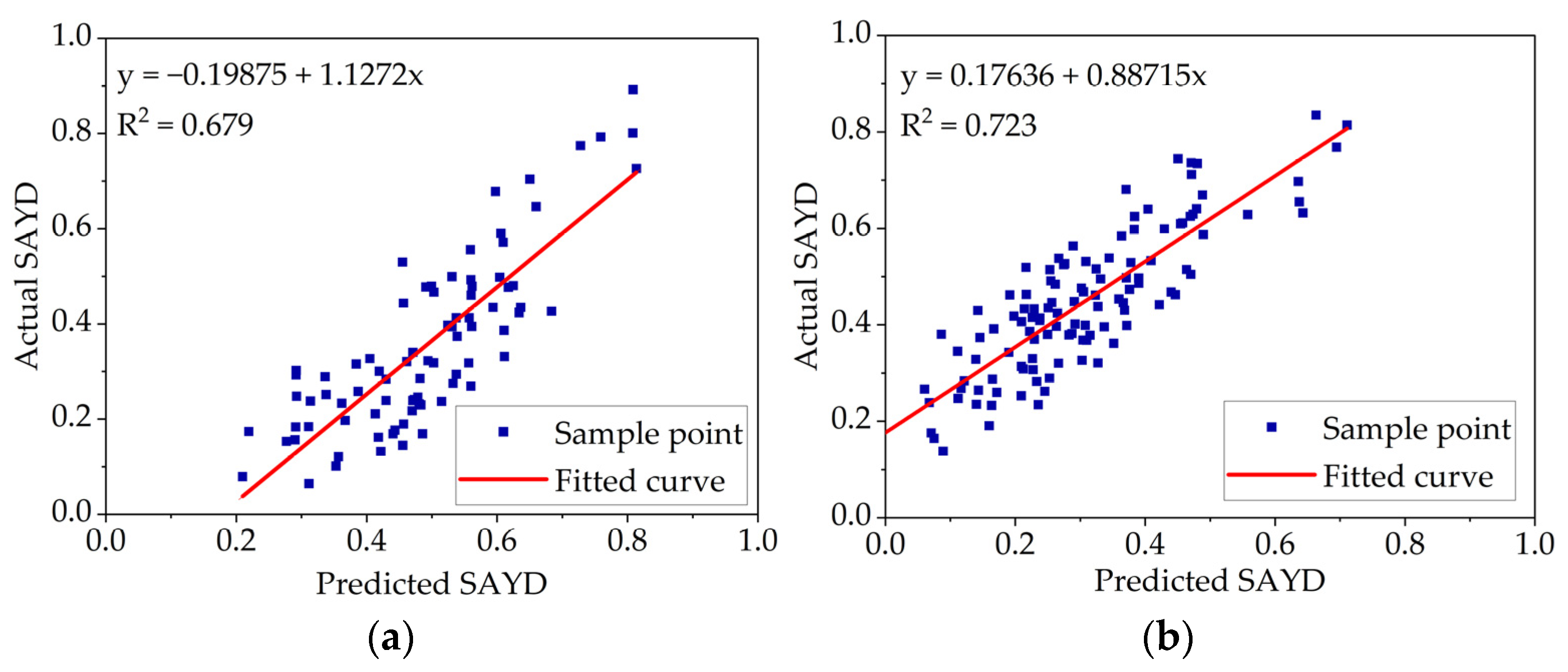
The fitted model parameters for SAYD and CT in regions A and B are shown in Table 4: validation of the non-linear model built in region A using areca tree data from region B and validation of the non-linear model built in region B using areca tree data from region A. The results are shown in Figure 10. The model is shown in Equation (9). The results show that the SAYD is closely related to its CT within the same period.
4. Discussion
4.1. Machine Learning in Areca YLD Prediction
By comparing the classification accuracy of the six classification models built in the study for areca YLD, the results are shown in Table 3. It is found that the RF algorithm outperforms the other five algorithms in classification. DT has only a single output, which can lead to overfitting and a poor performance when dealing with data with a relatively strong feature correlation [57]. The RF contains multiple decision trees, and the plurality of the categories output by each tree determines its output category, compared with a single DT; even though individual decision trees may lead to inaccurate predictions due to the influence of outliers, the prediction results are obtained by referring to multiple decision trees, reducing the influence caused by outliers [54], and therefore, RF will be more effective in classifying areca YLD compared to a single DT. NN and SVM are relatively good at classification. This is mainly because NN is adaptive and can be trained to adapt to changes in data species and noise, and they can handle non-linear problems well [50]; SVM avoids the complexity of high-dimensional space and directly uses the kernel function of this space and then directly solves the decision problem in the corresponding high dimensional space using the solution method in the linearly divisible case [52]. NB assumes that the attributes are independent, and this assumption is often not valid in practical applications [51]. Areca YLD has many correlated eigenvalues, so the classification effect is relatively less effective. KNN has no assumptions about the data and is insensitive to outliers compared to NB. However, it has high computational complexity and memory consumption because for each text to be classified, the distance from it to all known samples is computed to find its Kth nearest neighbors [53]. Therefore, although the accuracy of the KNN classification is relatively high, there are better choices for classifying areca YLD. In addition, only the prediction effect of some classification learning algorithms on areca YLD has been discussed. In the future, the prediction effect of deep learning algorithms on areca YLD can be studied, and the SAYD can be predicted directly to further improve the monitoring efficiency of areca YLD.
4.2. Feature Selection in Areca YLD Prediction
Lei S. [16] and others used the UAV multispectral remote sensing method to monitor areca YLD, selecting NDVI, OSAVI, LCI, GNDVI, and NDRE index as feature values and establishing back propagation neural networks, DT, NB, SVM, and KNN classifications, as five algorithmic models, and the classification accuracy reached 86.57%. However, a small number of vegetation indices could not stably and accurately characterize the characteristics of yellowed leaves, which limited the accuracy of the model. This study uses the ReliefF feature selection algorithm to filter out ten feature values associated with areca YLD, significantly improving the model classification accuracy. Compared to the results derived from Lei S’s work [16], the feature preference method proposed in this study has significantly improved in accuracy and the Kappa index, in which the accuracy of NN has improved by 0.119 and the Kappa index by 0.238; the accuracy of DT has improved by 0.130 and the Kappa index by 0.261; the accuracy of NB has improved by 0.104 and the Kappa index by 0.207; the accuracy of SVM has improved by 0.121 and the Kappa index by 0.247; the accuracy of KNN has improved by 0.165 and the Kappa index by 0.333. In addition, this study also uses the RF algorithm to build the model, and the effectiveness of the classification is further improved. Thus, it can be said that this study is a further improvement of this literature [16].
4.3. CT and Vegetation Indexes’ Relevance Analysis in Areca YLD Prediction
From Figure 9, it can be found that SAYD has a strong positive correlation with CI, NDRE, and LCI (0.911, 0.897, 0.790; p values < 0.001); CI and LCI were closely related to chlorophyll content [31,44], and it is clear that there is also a strong correlation between the SAYD and chlorophyll content. There was a strong negative correlation between SAYD and CLSI (−0.934; p values < 0.001), a vegetation index based on reflectance at a narrow band centered at 700 nm [33]. As Gitelson and Merzlyak [58] pointed out, reflectance near 700 nm is a fundamental feature of green vegetation produced by an equilibrium between biochemical and biophysical plant characteristics. The blue shift of the reflectance curve’s red edge frequently accompanies stress [59,60]. It could provide early detection of plant stress for most causes of stress, and the effectiveness of the reflectance of areca canopies near 700 nm for detecting YLD could be investigated in the future [33].
Previous related literature shows that thermal infrared imaging technology has excellent potential for application in remote sensing monitoring [61]. When crops receive infections such as fungi and pathogens, the cell membrane permeability increases, water loss is accelerated, and plants experience water loss and wilting [62]. At the same time, leaf stomatal heterogeneity closes, and the degree of heat loss from the leaf surface changes, resulting in a foliar temperature response. The changes in thermal radiation energy caused by water loss, stomatal closure, and enhanced plant respiration after crop disease can be visualized on a thermal infrared map [63]. Figure 9 shows that SAYD has a strong positive correlation with CT (0.753; p values < 0.001), demonstrating a strong correlation between SAYD and areca CT at the same ambient temperature. To test this idea, we built two non-linear models to predict SAYD by CT and cross-validated them with an R2 of 0.723. Therefore, in the future, the SAYD in an areca forest can be predicted by a UAV with an H20T sensor, which is less affected by light than visible light sensors for SAYD monitoring, which can work all day long and has a better penetration capacity. In addition, the low correlation between SAYD and CT may have been influenced by the prevailing weather and the quality of the UAV imaging. Other reasons may be that the CT acquisition was radiometrically corrected using only water temperature, and the inclusion of a variety of calibration plates with different reflectivity to assist in radiometric calibration may have increased the accuracy of the CT acquisition, which requires further validation. This study did not verify the correlation between SAYD and CT at different ambient temperatures, and multiple controlled experiments could be designed to verify this result.
4.4. Contributions and Limitations in the Method
This study provides a feasible and effective new method for monitoring the YLD of areca and improves the accuracy of monitoring SAYD. Compared with the traditional visual observation method, the method proposed can help farmers to monitor the distribution of SAYD in real-time at a lower cost and prescribe the right medicine for the right problem, thus effectively reducing drug abuse and helping areca YLD research teams to monitor SAYD better. The result verifies that SAYD is highly positively correlated with its CT at the same environmental temperature, but there is no such conclusion in previous studies. The reason may be that the average height of the areca tree is high, so it is not easy to measure its CT by a manual method. The areca canopy temperature was obtained using UAV equipped with thermal infrared sensors, and the high flux temperature of the areca canopy was obtained. The conclusion enables farmers to choose a cheaper thermal infrared sensor to monitor SAYD instead of an expensive multi-spectral sensor, which saves the cost of monitoring SAYD. At the same time, it also provides a new direction for the areca YLD research team to study areca YLD and broadens the research ideas of areca YLD.
There are still some limitations in the monitoring method of SAYD, which need to be further verified and improved. In this study, the ReliefF feature selection algorithm and different machine learning classification algorithms are used to improve the monitoring accuracy of SAYD significantly. The results show that the monitoring model of SAYD based on the ReliefF-RF algorithm performs better than other models. Previous studies have shown that artificial neural networks (ANNs) can predict the area under the disease development curve of the tomato late blight pathological system [64]. The latest generation of convolutional neural networks (CNNs) can effectively identify 13 plant diseases and distinguish plant leaves from the surrounding environment [65]. Therefore, continuously evolving deep learning models, such as ANNs and CNNs, can be further studied to improve the performance of SAYD monitoring. This study verifies the correlation between SAYD and its CT under the same environmental temperature and similar period conditions; the conclusion needs to be further validated under various weather and climate conditions because of the relatively simple experimental condition settings. Previous research has shown that the relative values of canopy temperature between certain tree species are less affected by different environmental changes [66]. Especially for areca trees grown in tropical regions, the climate and environmental temperatures are relatively stable. The error in analyzing SAYD using multispectral data may mainly come from the influence of lighting during imaging. In the future, low-cost imaging sensors such as thermal infrared and visible light can be tested to conduct experiments under gradient setting environmental conditions to analyze the impact of different conditions on monitoring accuracy. Introducing the correction model based on spectral information may minimize the impact.
5. Conclusions
This study achieved the quantitative prediction of areca YLD using a UAV platform equipped with a multi-source sensing system combined with a feature selection algorithm and machine learning algorithm. The experimental results showed the excellent accuracy of the method and demonstrated the correlation between CT and SAYD. The promotion of this method would help the relevant person to determine the degree and development trend of areca YLD more accurately and efficiently. In the future, with the development of sensors and deep learning technology, cheaper imaging devices such as visible light cameras, combined with high-performance post-processing algorithms, can be used to achieve intelligent monitoring of areca trees and even more plant diseases and pests at lower costs and more stable performances.
Author Contributions
Y.L. and L.Y. designed the research. D.X., H.L. and Z.L. performed the experiments. D.X. and Y.L. analyzed the data and wrote the manuscript. Q.L. and L.Y. supervised the project. All authors have read and agreed to the published version of the manuscript.
Funding
This research was funded by Hainan Yazhou Bay Seed Lab (B21HJ0904), Hainan Provincial Natural Science Foundation of China (322MS029).
Data Availability Statement
Data will be made available on request.
Conflicts of Interest
The authors declare that the research was conducted in the absence of any commercial or financial relationships that could be construed as a potential conflict of interest.
References
- Khan, L.U.; Cao, X.; Zhao, R.; Tan, H.; Xing, Z.; Huang, X. Effect of temperature on yellow leaf disease symptoms and its associated areca palm velarivirus 1 titer in areca palm (Areca catechu L.). Front. Plant Sci. 2022, 13, 1023386. [Google Scholar] [CrossRef] [PubMed]
- Peng, W.; Liu, Y.-J.; Wu, N.; Sun, T.; He, X.-Y.; Gao, Y.-X.; Wu, C.-J. Areca catechu L. (Arecaceae): A review of its traditional uses, botany, phytochemistry, pharmacology and toxicology. J. Ethnopharmacol. 2015, 164, 340–356. [Google Scholar] [CrossRef] [PubMed]
- Lee, S.E.; Hwang, H.J.; Ha, J.-S.; Jeong, H.-S.; Kim, J.H. Screening of medicinal plant extracts for antioxidant activity. Life Sci. 2003, 73, 167–179. [Google Scholar] [CrossRef]
- Zheng, W.; Li, X.-M.; Wang, F.; Yang, Q.; Deng, P.; Zeng, G.-M. Adsorption removal of cadmium and copper from aqueous solution by areca: A food waste. J. Hazard. Mater. 2008, 157, 490–495. [Google Scholar] [CrossRef] [PubMed]
- Sishodia, R.P.; Ray, R.L.; Singh, S.K. Applications of Remote Sensing in Precision Agriculture: A Review. Remote Sens. 2020, 12, 3136. [Google Scholar] [CrossRef]
- Wallace, L.; Lucieer, A.; Malenovsky, Z.; Turner, D.; Vopenka, P. Assessment of Forest Structure Using Two UAV Techniques: A Comparison of Airborne Laser Scanning and Structure from Motion (SfM) Point Clouds. Forests 2016, 7, 62. [Google Scholar] [CrossRef] [Green Version]
- Martin, C.; Parkes, S.; Zhang, Q.; Zhang, X.; McCabe, M.F.; Duarte, C.M. Use of unmanned aerial vehicles for efficient beach litter monitoring. Mar. Pollut. Bull. 2018, 131, 662–673. [Google Scholar] [CrossRef] [Green Version]
- Zhou, H.; Kong, H.; Wei, L.; Creighton, D.; Nahavandi, S. Efficient Road Detection and Tracking for Unmanned Aerial Vehicle. IEEE Trans. Intell. Transp. Syst. 2015, 16, 297–309. [Google Scholar] [CrossRef]
- Zhang, C.; Kovacs, J.M. The application of small unmanned aerial systems for precision agriculture: A review. Precis. Agric. 2012, 13, 693–712. [Google Scholar] [CrossRef]
- Franke, J.; Menz, G.; Oerke, E.-C.; Rascher, U. Comparison of multi- and hyperspectral imaging data of leaf rust infected wheat plants. In Remote Sensing for Agriculture, Ecosystems, and Hydrology VII; SPIE: Bellingham, DC, USA, 2005. [Google Scholar]
- Jiang, J.-B.; Huang, W.-J.; Chen, Y.-H. Using Canopy Hyperspectral Ratio Index to Retrieve Relative Water Content of Wheat under Yellow Rust Stress. Spectrosc. Spectr. Anal. 2010, 30, 1939–1943. [Google Scholar] [CrossRef]
- Franceschini, M.H.D.; Bartholomeus, H.; van Apeldoorn, D.; Suomalainen, J.; Kooistra, L. Intercomparison of Unmanned Aerial Vehicle and Ground-Based Narrow Band Spectrometers Applied to Crop Trait Monitoring in Organic Potato Production. Sensors 2017, 17, 1428. [Google Scholar] [CrossRef] [PubMed] [Green Version]
- Abdulridha, J.; Ampatzidis, Y.; Qureshi, J.; Roberts, P. Laboratory and UAV-Based Identification and Classification of Tomato Yellow Leaf Curl, Bacterial Spot, and Target Spot Diseases in Tomato Utilizing Hyperspectral Imaging and Machine Learning. Remote Sens. 2020, 12, 2732. [Google Scholar] [CrossRef]
- Chang, A.; Yeom, J.; Jung, J.; Landivar, J. Comparison of Canopy Shape and Vegetation Indices of Citrus Trees Derived from UAV Multispectral Images for Characterization of Citrus Greening Disease. Remote Sens. 2020, 12, 4122. [Google Scholar] [CrossRef]
- Vanegas, F.; Bratanov, D.; Powell, K.; Weiss, J.; Gonzalez, F. A Novel Methodology for Improving Plant Pest Surveillance in Vineyards and Crops Using UAV-Based Hyperspectral and Spatial Data. Sensors 2018, 18, 260. [Google Scholar] [CrossRef] [PubMed] [Green Version]
- Lei, S.; Luo, J.; Tao, X.; Qiu, Z. Remote Sensing Detecting of Yellow Leaf Disease of Arecanut Based on UAV Multisource Sensors. Remote Sens. 2021, 13, 4562. [Google Scholar] [CrossRef]
- Calderon, R.; Navas-Cortes, J.A.; Lucena, C.; Zarco-Tejada, P.J. High-resolution airborne hyperspectral and thermal imagery for early, detection of Verticillium wilt of olive using fluorescence, temperature and narrow-band spectral indices. Remote Sens. Environ. 2013, 139, 231–245. [Google Scholar] [CrossRef]
- Zhang, J.; Huang, Y.; Pu, R.; Gonzalez-Moreno, P.; Yuan, L.; Wu, K.; Huang, W. Monitoring plant diseases and pests through remote sensing technology: A review. Comput. Electron. Agric. 2019, 165, 104943. [Google Scholar] [CrossRef]
- Smigaj, M.; Gaulton, R.; Suarez, J.C.; Barr, S.L. Canopy temperature from an Unmanned Aerial Vehicle as an indicator of tree stress associated with red band needle blight severity. For. Ecol. Manag. 2019, 433, 699–708. [Google Scholar] [CrossRef]
- Wang, Y.; Zia-Khan, S.; Owusu-Adu, S.; Miedaner, T.; Mueller, J. Early Detection of Zymoseptoria tritici in Winter Wheat by Infrared Thermography. Agriculture 2019, 9, 139. [Google Scholar] [CrossRef] [Green Version]
- Cheng, J.J.; Li, H.; Ren, B.; Zhou, C.J.; Kang, Z.S.; Huang, L.L. Effect of canopy temperature on the stripe rust resistance of wheat. N. Z. J. Crop Hortic. Sci. 2015, 43, 306–315. [Google Scholar] [CrossRef] [Green Version]
- Rumpf, T.; Mahlein, A.K.; Steiner, U.; Oerke, E.C.; Dehne, H.W.; Pluemer, L. Early detection and classification of plant diseases with Support Vector Machines based on hyperspectral reflectance. Comput. Electron. Agric. 2010, 74, 91–99. [Google Scholar] [CrossRef]
- Rouse, J.W.; Haas, R.H.; Deering, D.W.; Schell, J.A.; Harlan, J.C. Monitoring the Vernal Advancement and Retrogradation (Green Wave Effect) of Natural Vegetation; NASA Technical Reports Server (NTRS): Chicago, IL, USA, 1973.
- Verstraete, M.M.; Pinty, B.; Myneni, R.B. Potential and limitations of information extraction on the terrestrial biosphere from satellite remote sensing. Remote Sens. Environ. 1996, 58, 201–214. [Google Scholar] [CrossRef]
- Pearson, R.L.; Miller, L.D. Remote mapping of standing crop biomass for estimation of the productivity of the shortgrass prairie. Remote Sens. Environ. VIII 1972, 1355. [Google Scholar]
- Yang, C.-M.; Cheng, C.-H.; Chen, R.-K. Changes in Spectral Characteristics of Rice Canopy Infested with Brown Planthopper and Leaffolder. Crop Sci. 2007, 47, 329–335. [Google Scholar] [CrossRef]
- Zhao, C.; Huang, M.; Huang, W.; Liu, L.; Wang, J.J.I.I.I.G.; Symposium, R.S. Analysis of winter wheat stripe rust characteristic spectrum and establishing of inversion models. IEEE Int. Geosci. Remote Sens. Symp. 2004, 6, 4318–4320. [Google Scholar]
- Jordan, C.F.J.E. Derivation of Leaf-Area Index from Quality of Light on the Forest Floor. Ecology 1969, 50, 663–666. [Google Scholar] [CrossRef]
- Fitzgerald, G.; Rodriguez, D.; O’Leary, G. Measuring and predicting canopy nitrogen nutrition in wheat using a spectral index—The canopy chlorophyll content index (CCCI). Field Crops Res. 2010, 116, 318–324. [Google Scholar] [CrossRef]
- Rondeaux, G.; Steven, M.D.; Baret, F. Optimization of soil-adjusted vegetation indices. Remote Sens. Environ. 1996, 55, 95–107. [Google Scholar] [CrossRef]
- Penuelas, J.; Baret, F.; Filella, I. Semi-empirical indices to assess carotenoids/chlorophyll alpha ratio from leaf spectral reflectance. Photosynthetica 1995, 31, 221–230. [Google Scholar]
- Gitelson, A.A.; Merzlyak, M.N.; Chivkunova, O.B. Optical properties and nondestructive estimation of anthocyanin content in plant leaves. Photochem. Photobiol. 2001, 74, 38–45. [Google Scholar] [CrossRef]
- Mahlein, A.K.; Rumpf, T.; Welke, P.; Dehne, H.W.; Pluemer, L.; Steiner, U.; Oerke, E.C. Development of spectral indices for detecting and identifying plant diseases. Remote Sens. Environ. 2013, 128, 21–30. [Google Scholar] [CrossRef]
- Wang, Z.J.; Wang, J.H.; Liu, L.Y.; Huang, W.J.; Zhao, C.J.; Wang, C.Z. Prediction of grain protein content in winter wheat (Triticum aestivum L.) using plant pigment ratio (PPR). Field Crops Res. 2004, 90, 311–321. [Google Scholar] [CrossRef]
- Zarco-Tejada, P.J.; Berjón, A.; López-Lozano, R.; Miller, J.R.; Martín, P.; Cachorro, V.; González, M.R.; de Frutos, A. Assessing vineyard condition with hyperspectral indices: Leaf and canopy reflectance simulation in a row-structured discontinuous canopy. Remote Sens. Environ. 2005, 99, 271–287. [Google Scholar] [CrossRef]
- Haboudane, D.; Miller, J.R.; Tremblay, N.; Zarco-Tejada, P.J.; Dextraze, L. Integrated narrow-band vegetation indices for prediction of crop chlorophyll content for application to precision agriculture. Remote Sens. Environ. 2002, 81, 416–426. [Google Scholar] [CrossRef]
- Naidu, R.A.; Perry, E.M.; Pierce, F.J.; Mekuria, T. The potential of spectral reflectance technique for the detection of Grapevine leafroll-associated virus-3 in two red-berried wine grape cultivars. Comput. Electron. Agric. 2009, 66, 38–45. [Google Scholar] [CrossRef]
- Merzlyak, M.N.; Gitelson, A.A.; Chivkunova, O.B.; Rakitin, V.Y. Non-destructive optical detection of pigment changes during leaf senescence and fruit ripening. Physiol. Plant. 1999, 106, 135–141. [Google Scholar] [CrossRef] [Green Version]
- Qi, J.; Chehbouni, A.; Huete, A.R.; Kerr, Y.H.; Sorooshian, S. A modified soil adjusted vegetation index. Remote Sens. Environ. 1994, 48, 119–126. [Google Scholar] [CrossRef]
- Chen, S.F.; Goodman, J. An empirical study of smoothing techniques for language modeling. Comput. Speech Lang. 1999, 13, 359–394. [Google Scholar] [CrossRef] [Green Version]
- Gamon, J.A.; Peñuelas, J.; Field, C.B. A narrow-waveband spectral index that tracks diurnal changes in photosynthetic efficiency. Remote Sens. Environ. 1992, 41, 35–44. [Google Scholar] [CrossRef]
- Huete, A.R. A soil-adjusted vegetation index (SAVI). Remote Sens. Environ. 1988, 25, 295–309. [Google Scholar] [CrossRef]
- Gitelson, A.A. Wide Dynamic Range Vegetation Index for remote quantification of biophysical characteristics of vegetation. J. Plant Physiol. 2004, 161, 165–173. [Google Scholar] [CrossRef] [PubMed] [Green Version]
- Gitelson, A.A.; Viña, A.; Ciganda, V.; Rundquist, D.C.; Arkebauer, T.J. Remote estimation of canopy chlorophyll content in crops. Geophys. Res. Lett. 2005, 32. [Google Scholar] [CrossRef] [Green Version]
- Liu, M.; Luo, Y.; Tao, D.; Xu, C.; Wen, Y. Low-Rank Multi-View Learning in Matrix Completion for Multi-Label Image Classification. In Proceedings of the AAAI Conference on Artificial Intelligence, Austin, TX, USA, 25–30 January 2015. [Google Scholar]
- Robnik-Šikonja, M.; Kononenko, I. Theoretical and Empirical Analysis of ReliefF and RReliefF. Mach. Learn. 2003, 53, 23–69. [Google Scholar] [CrossRef] [Green Version]
- Kira, K.; Rendell, L.A. A Practical Approach to Feature Selection. In Machine Learning Proceedings 1992; Sleeman, D., Edwards, P., Eds.; Morgan Kaufmann: San Francisco, CA, USA, 1992; pp. 249–256. [Google Scholar]
- Kononenko, I. Estimating Attributes: Analysis and Extensions of RELIEF; ECML: Berlin/Heidelberg, Germany, 1994; pp. 171–182. [Google Scholar]
- Messina, G.; Modica, G. Applications of UAV Thermal Imagery in Precision Agriculture: State of the Art and Future Research Outlook. Remote Sens. 2020, 12, 1491. [Google Scholar] [CrossRef]
- Lassoued, H.; Ketata, R. ECG multi-class classification using neural network as machine learning model. In Proceedings of the 2018 International Conference on Advanced Systems and Electric Technologies (IC_ASET), Hammamet, Tunisia, 22–25 March 2018; pp. 473–478. [Google Scholar]
- Rish, I. An empirical study of the naive Bayes classifier. IJCAI 2001 Workshop Empir. Methods Artif. Intell. 2001, 3, 41–46. [Google Scholar]
- Awad, M.; Khanna, R. Support Vector Machines for Classification. In Efficient Learning Machines; Apress: Berkeley, CA, USA, 2015; pp. 39–66. [Google Scholar]
- Cover, T.M.; Hart, P.E.J.I.T.I.T. Nearest neighbor pattern classification. IEEE Trans. Inf. Theory 1967, 13, 21–27. [Google Scholar] [CrossRef] [Green Version]
- Breiman, L. Random Forests. Mach. Learn. 2001, 45, 5–32. [Google Scholar] [CrossRef] [Green Version]
- Sokolova, M.; Lapalme, G. A systematic analysis of performance measures for classification tasks. Inf. Process. Manag. 2009, 45, 427–437. [Google Scholar] [CrossRef]
- Viera, A.J.; Garrett, J.M. Understanding interobserver agreement: The kappa statistic. Fam. Med. 2005, 37, 360–363. [Google Scholar]
- Loh, W.-Y. Classification and Regression Trees. Wiley Interdiscip. Rev. Data Min. Knowl. Discov. 2011, 1, 14–23. [Google Scholar] [CrossRef]
- Gitelson, A.A.; Merzlyak, M.N. Remote estimation of chlorophyll content in higher plant leaves. Int. J. Remote Sens. 1997, 18, 2691–2697. [Google Scholar] [CrossRef]
- Carter, G.A.; Miller, R.L. Early detection of plant stress by digital imaging within narrow stress-sensitive wavebands. Remote Sens. Environ. 1994, 50, 295–302. [Google Scholar] [CrossRef]
- Gitelson, A.; Merzlyak, M.N. Spectral Reflectance Changes Associated with Autumn Senescence of Aesculus hippocastanum L. and Acer platanoides L. Leaves. Spectral Features and Relation to Chlorophyll Estimation. J. Plant Physiol. 1994, 143, 286–292. [Google Scholar] [CrossRef]
- Ippalapally, R.; Mudumba, S.H.; Adkay, M.; HR, N.V. Object Detection Using Thermal Imaging. In Proceedings of the 2020 IEEE 17th India Council International Conference (INDICON), New Delhi, India, 10–13 December 2020; pp. 1–6. [Google Scholar]
- Durner, J.; Klessig, D.F. Salicylic Acid Is a Modulator of Tobacco and Mammalian Catalases. J. Biol. Chem. 1996, 271, 28492–28501. [Google Scholar] [CrossRef] [Green Version]
- Jones, H.G.; Serraj, R.; Loveys, B.R.; Xiong, L.; Wheaton, A.; Price, A.H. Thermal infrared imaging of crop canopies for the remote diagnosis and quantification of plant responses to water stress in the field. Funct. Plant Biol. FPB 2009, 36, 978–989. [Google Scholar] [CrossRef] [Green Version]
- Alves, D.P.; Tomaz, R.S.; Laurindo, B.S.; Laurindo, R.D.F.; Silva, F.F.E.; Cruz, C.D.; Nick, C.; da Silva, D.J.H. Artificial neural network for prediction of the area under the disease progress curve of tomato late blight. Sci. Agric. 2017, 74, 51–59. [Google Scholar] [CrossRef] [Green Version]
- Sladojevic, S.; Arsenovic, M.; Anderla, A.; Culibrk, D.; Stefanovic, D. Deep Neural Networks Based Recognition of Plant Diseases by Leaf Image Classification. Comput. Intell. Neurosci. 2016, 2016, 3289801. [Google Scholar] [CrossRef] [Green Version]
- Saito, T.; Kumagai, T.O.; Tateishi, M.; Kobayashi, N.; Otsuki, K.; Giambelluca, T.W. Differences in seasonality and temperature dependency of stand transpiration and canopy conductance between Japanese cypress (Hinoki) and Japanese cedar (Sugi) in a plantation. Hydrol. Process. 2017, 31, 1952–1965. [Google Scholar] [CrossRef]
Figure 1.
Technical route of the research.

Figure 2.
Overview of the research area.

Figure 3.
Schematic diagram of the classification algorithm: (a) neural network; (b) naïve Bayes; (c) support vector machine; (d) K nearest-neighbors; (e) decision tree; (f) random forest.
Figure 3.
Schematic diagram of the classification algorithm: (a) neural network; (b) naïve Bayes; (c) support vector machine; (d) K nearest-neighbors; (e) decision tree; (f) random forest.


Figure 4.
Areca zoning in the study area.
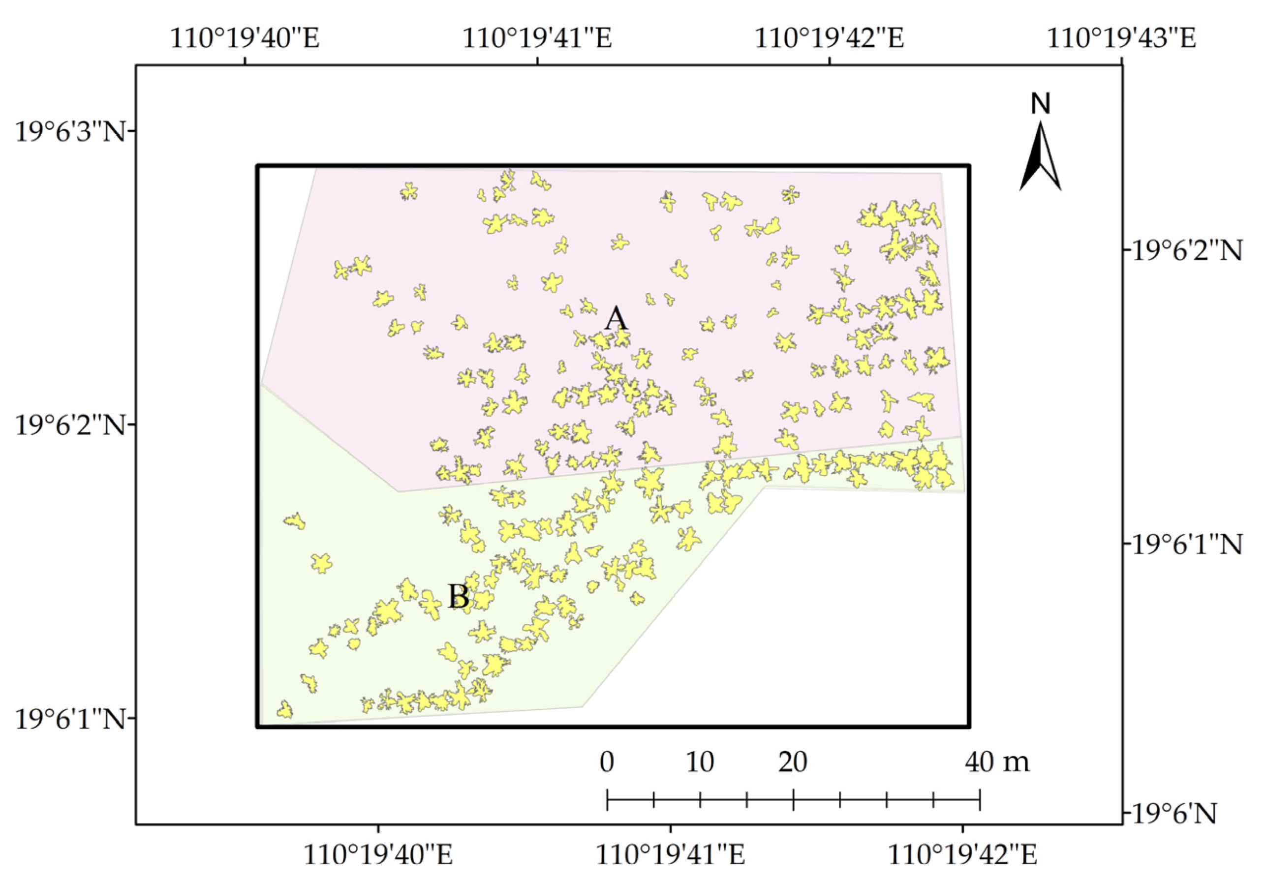
Figure 5.
Relationship between the number of feature variables and the accuracy rate.
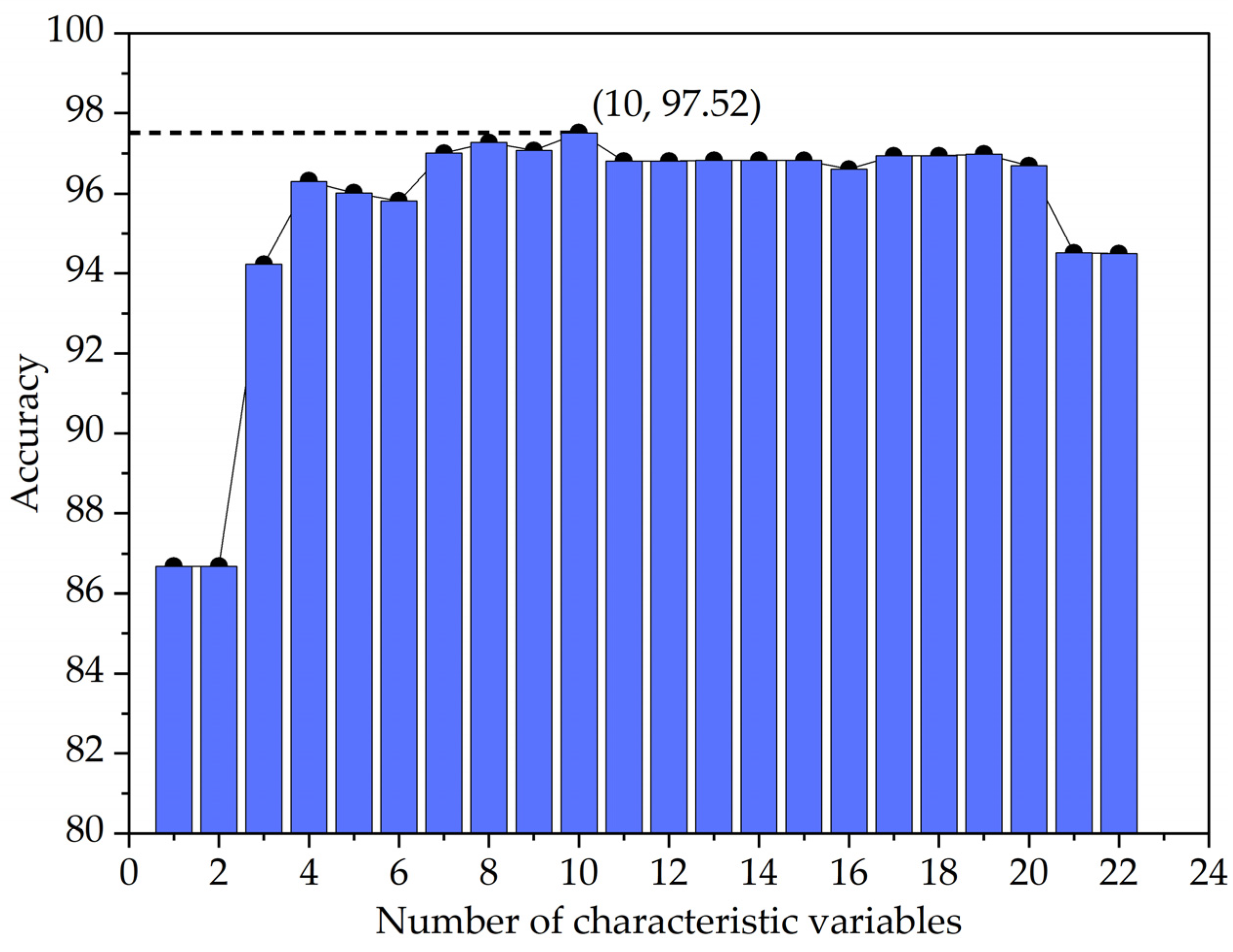
Figure 6.
Spatial distribution map of SAYD based on six machine learning models: (a) NN; (b) NB; (c) SVM; (d) KNN; (e) DT; (f) RF.
Figure 6.
Spatial distribution map of SAYD based on six machine learning models: (a) NN; (b) NB; (c) SVM; (d) KNN; (e) DT; (f) RF.

Figure 7.
Correlation between SAYD based on the ReliefF-RF model and actual values.
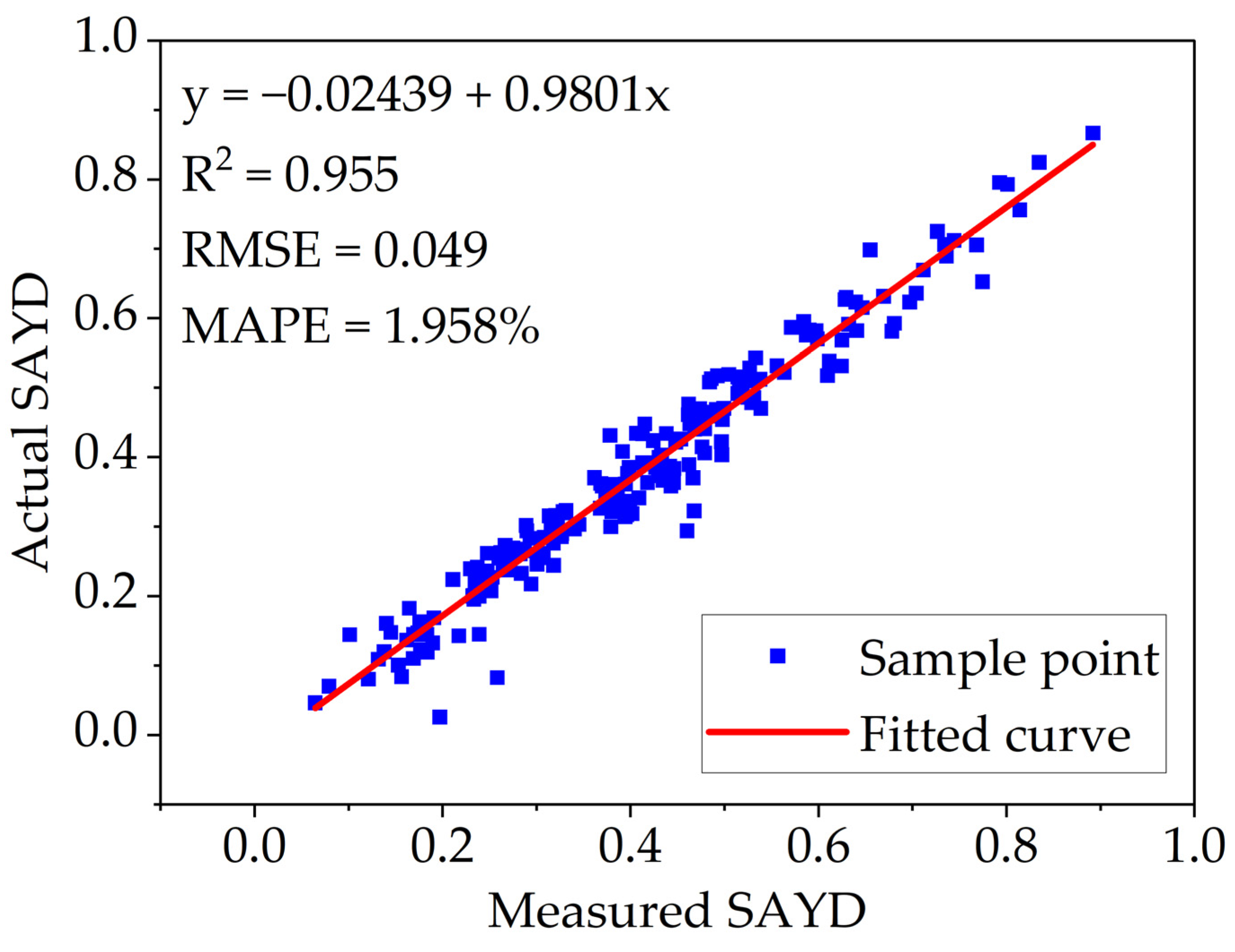
Figure 8.
Canopy temperature distribution of areca in the study area.
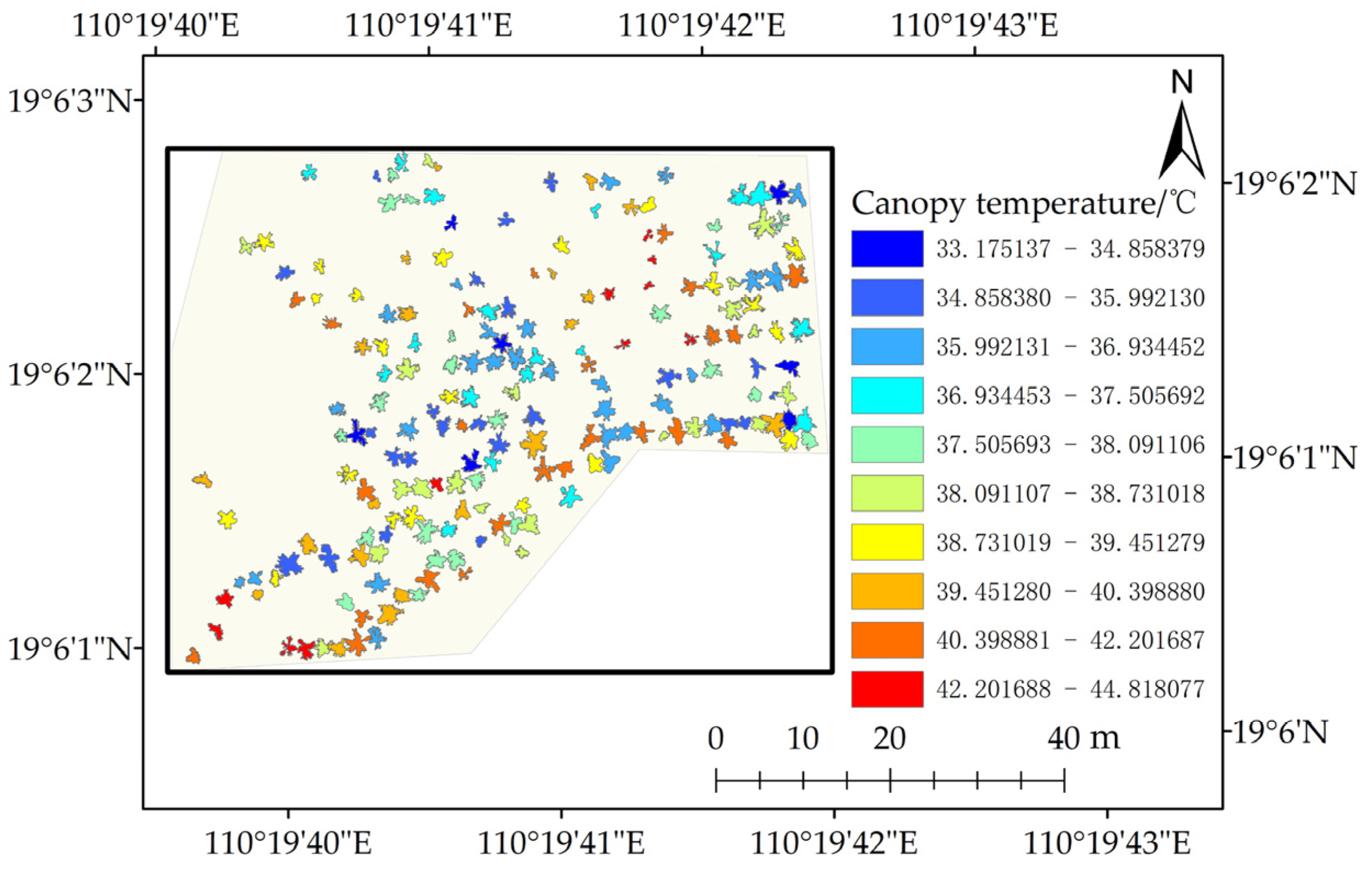
Figure 9.
Pearson’s correlation matrix for traits associated with areca YLD.
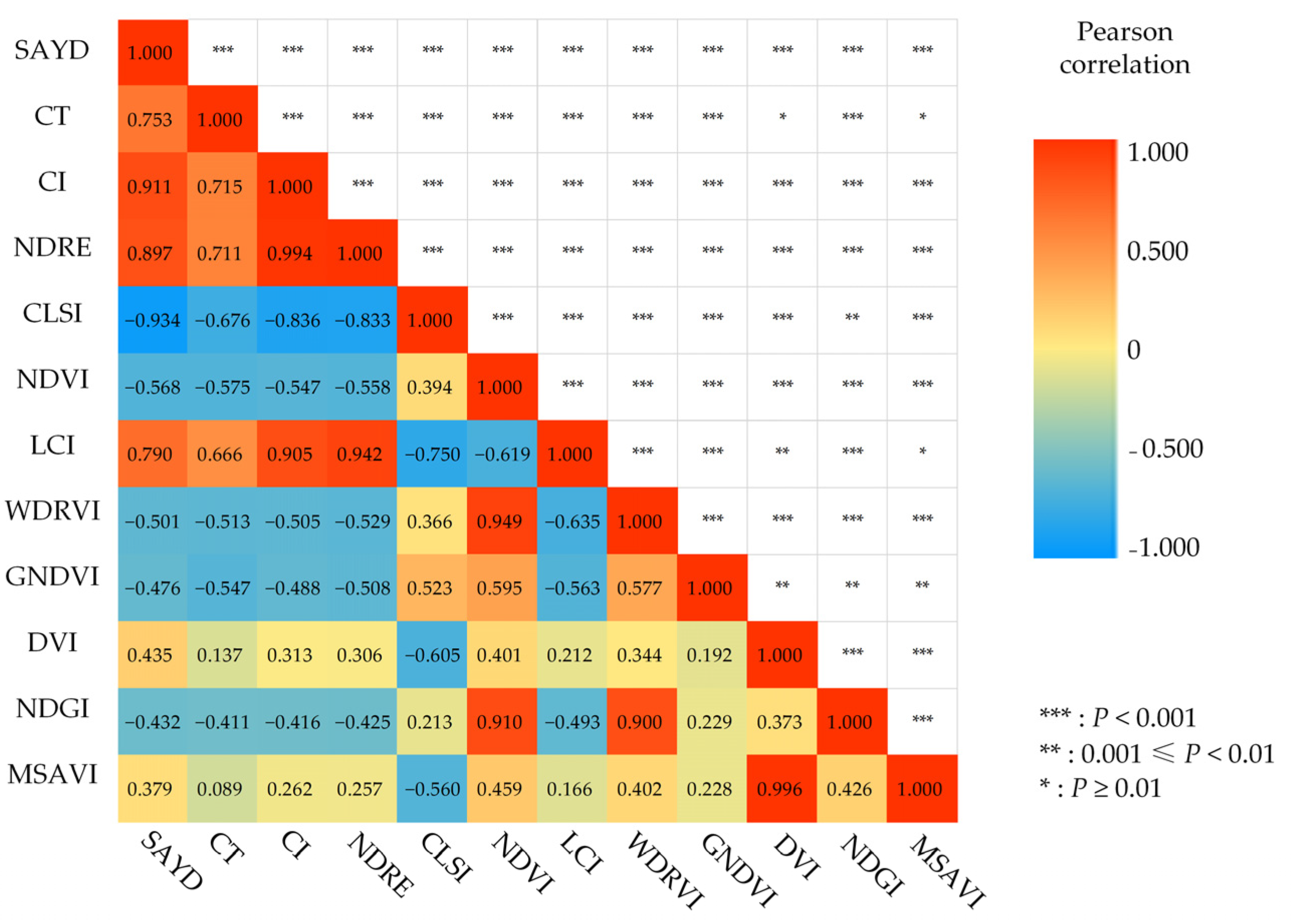
Figure 10.
Accuracy evaluation of SAYD and CT model: (a) validation of the model built in region A with data from region B; (b) validation of the model built in region B with data from region A.
Figure 10.
Accuracy evaluation of SAYD and CT model: (a) validation of the model built in region A with data from region B; (b) validation of the model built in region B with data from region A.

Table 1.
Multispectral vegetation index.
| Vegetation Index | Computing Formula | References |
|---|---|---|
| Normalized Difference Vegetation Index (NDVI) | NDVI = (RNIR − RRed)/(RNIR + RRed) | [23] |
| Enhanced Vegetation Index (EVI) | EVI = 2.5 × (RNIR − RRed)/(RNIR + 6 × RRed − 7.5 × RBlue + 1) | [24] |
| Ratio Vegetation Index (RVI) | RVI = RNIR/RRed | [25] |
| Green Normalized Difference Vegetation Index (GNDVI) | GNDVI = (RNIR − RGreen)/(RNIR + RGreen) | [26] |
| Triangle Vegetation Index (TVI) | TVI = 60 × (RNIR − RGreen) − 100 × (RRed − RGreen) | [27] |
| Difference Vegetation Index (DVI) | DVI = RNIR − RRed | [28] |
| Normalized Difference of Red Edge (NDRE) | NDRE = (RNIR − RRededge)/(RNIR + RRededge) | [29] |
| Optimized Soil-Adjusted Vegetation Index (OSAVI) | OSAVI = 1.16 × (RNIR − RRed)/(RNIR + RRed + 0.16) | [30] |
| Leaf Chlorophyll Index (LCI) | LCI = (RNIR − RRededge)/(RNIR + RRed) | [31] |
| Anthocyanin Reflection Index (ARI) | ARI = (1/RGreen) − (1/RRed) | [32] |
| Cercospora Leaf Spot Index (CLSI) | CLSI = (RRededge − RGreen)/(RRededge + RGreen) − RRededge | [33] |
| Plant Pigment Radio (PPR) | PPR = (RGreen − RBlue)/(RGreen + RBlue) | [34] |
| Greenness Index (GI) | GI = RGreen/RRed | [35] |
| Transformed Chlorophyll Absorption in Reflectance Index (TCARI) | TCARI = 3 × [(RNIR − RRed) − 0.2 × (RNIR − RGreen) × RNIR/RRed] | [36] |
| Visible light Atmospheric Rated impedance Index (VARI) | VARI = (RGreen − RRed)/(RGreen + RRed − RBlue) | [37] |
| Plant Senescence Reflectance Index (PSRI) | PSRI = (RRed − RGreen)/RNIR | [38] |
| Modified Soil and Adjusted Vegetation Index (MSAVI) | ] | [39] |
| Modified Simple Ratio Index (MSR) | [40] | |
| Normalized Difference Greenness Index (NDGI) | NDGI = (RGreen − RRed)/(RGreen + RRed) | [41] |
| Soil Adjusted Vegetation Index (SAVI) | SAVI = 1.5 × (RNIR − RRed)/(RNIR + RRed + 0.5) | [42] |
| Wide Dynamic Range Vegetation Index (WDRVI) | WDRVI = (0.1 × RNIR-RRed)/(0.1 × RNIR + RRed) | [43] |
| Red edge Chlorophyll Index (CI) | CI = (RNIR/RRededge) − 1 | [44] |
RBlue, RGreen, RRed, RNIR, and RRededge are the Multispectral sensor blue, green, red, near-infrared, and red-edge band reflectance, respectively.
Table 2.
Model parameter setting.
| Model | Parameter Setting |
|---|---|
| ReliefF | K: 10 |
| Expand setting: method-classification | |
| NN | Number of fully connected layers: 1 |
| First layer size: 10 | |
| Activation: ReLU | |
| Iteration limit: 1000 | |
| Regularization strength (lambda): 0 | |
| Standardize data: Yes | |
| NB | Distribution name for numeric predictors: Kernel |
| Distribution name for categorical predictors: Not Applicable | |
| Kernel type: Gaussian | |
| Support: Unbounded | |
| SVM | Kernel function: Gaussian |
| Kernel scale: 0.79 | |
| Box constraint level: 1 | |
| Multiclass method: One-vs-One | |
| Standardize data: true | |
| KNN | Number of neighbors: 1 |
| Distance metric: Euclidean | |
| Distance weights: Equal distance | |
| Standardize data: true | |
| DT | Maximum number of splits: 100 |
| Split criterion: Gini’s diversity index | |
| Surrogate decision splits: Off | |
| RF | Number of trees: 1000 |
| Maximum depth: 5 | |
| Minimum number of samples separated: 5 | |
| Minimum number of samples on leaf nodes after separation: 4 | |
| Number of features: auto |
Table 3.
Classification results of SAYD on a test set by different classification models.
| Model | Accuracy | Precision | Recall | F1 | Kappa |
|---|---|---|---|---|---|
| NN | 0.985 | 0.984 | 0.990 | 0.987 | 0.968 |
| NB | 0.940 | 0.940 | 0.958 | 0.949 | 0.877 |
| SVM | 0.984 | 0.983 | 0.990 | 0.986 | 0.967 |
| KNN | 0.977 | 0.977 | 0.985 | 0.981 | 0.953 |
| DT | 0.977 | 0.978 | 0.983 | 0.980 | 0.951 |
| RF | 0.987 | 0.990 | 0.988 | 0.989 | 0.972 |
Note: The bolded areas are the highest values in the column.
Table 4.
Fitting model parameters for regions A and B.
| Region | a | b |
|---|---|---|
| A | 8.16895 | −0.29052 |
| B | 9.20805 | −0.28432 |
Disclaimer/Publisher’s Note: The statements, opinions and data contained in all publications are solely those of the individual author(s) and contributor(s) and not of MDPI and/or the editor(s). MDPI and/or the editor(s) disclaim responsibility for any injury to people or property resulting from any ideas, methods, instructions or products referred to in the content. |
© 2023 by the authors. Licensee MDPI, Basel, Switzerland. This article is an open access article distributed under the terms and conditions of the Creative Commons Attribution (CC BY) license (https://creativecommons.org/licenses/by/4.0/).
Share and Cite
MDPI and ACS Style
Xu, D.; Lu, Y.; Liang, H.; Lu, Z.; Yu, L.; Liu, Q. Areca Yellow Leaf Disease Severity Monitoring Using UAV-Based Multispectral and Thermal Infrared Imagery. Remote Sens. 2023, 15, 3114. https://doi.org/10.3390/rs15123114
AMA Style
Xu D, Lu Y, Liang H, Lu Z, Yu L, Liu Q. Areca Yellow Leaf Disease Severity Monitoring Using UAV-Based Multispectral and Thermal Infrared Imagery. Remote Sensing. 2023; 15(12):3114. https://doi.org/10.3390/rs15123114
Chicago/Turabian StyleXu, Dong, Yuwei Lu, Heng Liang, Zhen Lu, Lejun Yu, and Qian Liu. 2023. "Areca Yellow Leaf Disease Severity Monitoring Using UAV-Based Multispectral and Thermal Infrared Imagery" Remote Sensing 15, no. 12: 3114. https://doi.org/10.3390/rs15123114
Note that from the first issue of 2016, this journal uses article numbers instead of page numbers. See further details here.