Article

Predicting Spatially Explicit Composite Burn Index (CBI) from Different Spectral Indices Derived from Sentinel 2A: A Case of Study in Tunisia

1
Institut Sylvo-Pastoral de Tabarka, Laboratoire des Ressources SYLVO-Pastorales, Université de Jendouba, Jendouba 8110, Tunisia
2
Department of Environmental Sciences, University of Castilla-La Mancha, Avd. Carlos III, s/n., 45071 Toledo, Spain
*
Author to whom correspondence should be addressed.
Remote Sens. 2023, 15(2), 335; https://doi.org/10.3390/rs15020335
Submission received: 5 December 2022 / Revised: 29 December 2022 / Accepted: 3 January 2023 / Published: 5 January 2023

Abstract

:
Fire severity, which quantifies the degree of organic matter consumption, is an important component of the fire regime. High-severity fires have major ecological implications, affecting carbon uptake, storage and emissions, soil nutrients, and plant regeneration, among other ecosystem services. Accordingly, spatially explicit maps of the fire severity are required to develop improved tools to manage and restore the most damaged areas. The aim of this study is to develop spatially explicit maps of the field-based fire severity (composite burn index—CBI) from different spectral indices derived from Sentinel 2A images and using several regression models. The study areas are two recent large fires that occurred in Tunisia in the summer of 2021. We employed different spectral severity indices derived from the normalized burn ratio (NBR): differenced NBR (dNBR), relative differenced NBR (RdNBR), and relativized burn Ratio (RBR). In addition, we calculated the burned area index for Sentinel 2 (BAIS2) and the thermal anomaly index (TAI). Different tree decision models (i.e., the recursive partitioning regression method [RPART], bagging regression trees [Bagging], and boosted regression trees [BRT]), as well as a generalized additive model [GAM]), were applied to predict the CBI. The main results indicated that RBR, followed by dNBR, were the most important spectral severity indices for predicting the field-based CBI. Moreover, BRT was the best regression model, explaining 92% of the CBI variance using the training set of points and 88% when using the validation set. These results suggested the adequacy of RBR index derived from Sentinel 2A for assessing and mapping forest fire severity in Mediterranean forests. These spatially explicit maps of field-based CBI could help improve post-fire recovery and restoration efforts.

1. Introduction

In recent decades, the likelihood of large wildfires burning at high intensity has increased in many regions of the world because of prolonged droughts and global warming [1,2,3]. Such fires often result in a heterogeneous pattern of biomass consumption [1,4,5,6], which is of great importance as it impacts several ecosystems properties, such as vegetation, soils, biodiversity, and water quality [7,8,9,10]. However, there is little information regarding the spatial heterogeneity of biomass consumed and the underlying mechanisms that regulate this variability at different scales [5,6,11,12]. Fire severity reflects the impact of fires in terms of the amount of plant biomass consumed (BC) or combustion efficiency [13,14] and has no single metric [13,15]. Therefore, various measures taken in the field such as changes in crown volume, the minimum diameter of branches remaining after fire, tree mortality, bare soil exposure, ash deposition, etc., are used as proxies for severity [13,16,17]. However, obtaining this information based only on fieldwork is a complex and expensive task, and it does not allow for obtaining spatially explicit knowledge of combustion efficiency and its effects. An effective alternative to provide spatially explicit information at a lower cost consists of using satellite images. Accordingly, and to integrate different measures of post-fire effects, Key and Benson [18] developed the composite burnt index (CBI) as a field assessment of the post-fire normalized burn ratio (NBR) spectral index derived from Landsat imagery. The CBI was originally developed and applied in the forests of the Western US and is used by interagency burned area emergency restoration (BAER) teams nationwide. In practice, the CBI index is assessed visually in situ based on the amount of fuel burnt, the level of soil carbonization, as well as the degree of vegetation recovery [18,19]. Five post-fire strata are assessed in 30 × 30 m plots: (1) substrate (material lying on the ground); (2) grasses, short shrubs, and small trees (<1 m tall); (3) tall shrubs and young trees (<5 m tall); (4) intermediate trees (5–20 m tall); and (5) large trees (>20 m tall). Assessments are made individually and then combined to obtain an overall CBI value at the plot level.
Although the CBI protocol is often used to assess the severity of forest fires, it has been criticized mainly because it does not consider differences in the percentage cover of vegetation strata [20,21]. As an alternative, De Santis and Chuvieco [22] suggested a modified version of the CBI, the so-called geometrically structured composite burn index (GeoCBI), which additionally integrates the percentage cover of each vegetation layer to improve the relationship between the CBI and the spectral severity index. In addition, some researchers in North America have proposed the weighted composite burn index (WCBI) as an alternative to the CBI. Unlike the CBI, the WCBI integrates the influences of the different vegetation strata by weighting them according to their percentage cover [20]. However, as suggested by Gallagher et al. [23], the fact that post-fire percent cover is often estimated visually can introduce a bias into the calculations that is difficult to quantify.
Satellite-derived data is an important tool for estimating fire severity regionally as changes in moisture and chlorophyll content of vegetation result in large changes in reflectance. Indeed, a fire-induced decrease in chlorophyll and moisture in vegetation leads to a decrease in visible (VIS) and near-infrared (NIR) reflectance and an increase in short-wave infrared (SWIR) reflectance [24]. In this context, several spectral indices derived from remote sensing data have been used to assess fire severity in different ecosystems [5,6,20,25,26,27,28,29]. These indices differ by the combination of spectral bands used. There are spectral indices that combine the red-NIR spectrum, including the normalized difference vegetation index (NDVI) and the enhanced vegetation index (EVI), and spectral indices that combine the spectral range NIR-SWIR, including the burned area index (BAI), the char soil index (CSI), the thermal anomaly index (TAI), the normalized burn ratio (NBR) and its bitemporal indices, including the differenced normalized burn ratio (dNBR), the relative differenced normalized burn ratio (RdNBR), and the relativized burn ratio (RBR) [18,30,31,32,33]. In addition, some authors such as [34] have suggested that indices that integrate broader spectral bands, such as the burned area index for Sentinel 2 (BAIS2), are more suitable for fire severity assessment. Despite this wide range of spectral indices, the most used index in assessing wildfire severity is the NBR and its bitemporal counterparts [1,18,25,35].
The accuracy of those indices has been assessed by examining the correlation between the CBI index values obtained in the field and their counterparts obtained from each spectral index. With this in mind, the question of which models are best suited to relate these spectral indices to the CBI data was also explored. It has been shown that in some areas the second-order polynomial regressions outperformed linear models, given the non-linear behavior of CBI with respect to spectral data and signal saturation at high-severity levels [3,5,35,36]. However, in other ones, linear models worked rather well [26,37,38]. Finally, it should be highlighted that although there is a huge bulk of literature devoted to relating CBI based on spectral severity indices., there is much less research focused on estimating the accuracy of such models in the space creating spatially-explicit maps of the CBI predicted on such indices [39].
In this study, we proposed different severity indices derived from Sentinel images as well as different regression methods to develop spatially-explicit models that predict continuous CBI values in space. Moreover, and as far as we know, this approach is the first one applied in the South Mediterranean areas of North Africa. The performance of those spectral indices and regression methods was evaluated by calculating the adjustment (R2) between the predicted and the observed CBI and the root mean square error (RMSE). The main specific objectives of this study were: (i) to calculate various severity indices from pre- and post-fire Sentinel images (i.e., dNBR, RBR, dTAI and dBAIS2), (ii) to run different regression algorithms to predict the CBI based on previous spectral indices: recursive partitioning regression (RPART), regression trees based on bagging (Bagging), boosted regression trees (BRT), and generalized additive models (GAMs), (iii) to estimate which spectral index and regression method are the most accurate to predict the CBI, and, finally, (iv) to spatialize the predicted CBI over the entire study area. This study focuses on two forest fires registered between July and August 2021 in northern Tunisia.

2. Materials and Methods

2.1. Study Areas

The selected sites include two large fires registered in northern Tunisia between July and August 2021 (Figure 1).
The Fernana (F1) fire occurred at 1:30 p.m. on 11 August 2021 in Fernana locality (Fernana delegation, Jendouba governorate). The fire lasted for two consecutive days and burned about 1500 ha (Table 1). The fire caused considerable ecological and economic damage, but there were no human casualties thanks to the early evacuation of the inhabitants of the surrounded villages by the local authorities. The vegetation cover in the region is dominated by forest tree species (Quercus suber, Quercus canariensis, Pinus pinaster, Pinus pinea L., Olea europaea, Eucalyptus sp., and Cupressus), mixed with shrubs such as Pistacia lentiscus, Myrtus communis, Phillyrea angustifolia, Erica arborea, Arbutus unedo, Acacia cyanophylla, and Calicotome villosa (Figure 2). The low shrubland consists of Ampelodesmos mauritanicus. Fernana belongs to the subhumid bioclimatic stage with temperate winters. The maximum monthly temperature recorded that year was 40 °C with a weak rainfall of 3.3 mm and a maximum wind speed of 22.5 km/h. The elevation ranges between 306 m and 756 m a.s.l.
The Takrouna fire (F2) broke out in the village of Takrouna (Sakiet Sidi Youssef delegation, Le Kef governorate) in the late evening of 25 July 2021 (around 12:30) and burned about 3000 ha over four consecutive days. Like Fernana, this fire did not cost any lives. The burnt vegetation cover consists mainly of forest stratum dominated by Pinus halepensis and shrubs of Quercus coccifera, Smilax aspera, Cistus salviifolius, Pistacia lentiscus, Calicotome villosa, Cistus monspeliensis, Drimia maritime, and low shrub species of Ampelodesmos mauritanicus (Figure 2). In terms of climate, the region largely belongs to the sub-humid stage. In summer, the region is subject to hot and drying winds (sirocco) which facilitate the spread of fires. The maximum average temperature recorded during that year was about 38.6 °C, 5.84 mm of precipitation, and a wind speed of 18 km/h. The elevation ranges from 466 m to 960 m a.s.l. Takrouna is characterized by an intermixed wild urban interface with scattered housings directly intermingling with wild vegetation.

2.2. Data

2.2.1. Satellite Imagery and Pre-Processing

Sentinel 2A Multispectral Instrument (MSI) satellite imagery for both fires was downloaded from the USGS Earth Explorer platform (http://earthexplorer.usgs.gov/; accessed on 12 October 2021); as a level-1C product with 13 spectral bands. Scenes before and after the fires were selected as close as possible to the fire ignition dates, with minimal cloud cover (Table 2). Following Achour et al. [33], the Sentinel 2A bands were resampled to a 20 m pixel size using the nearest neighbor technique to later stitch the bands together. The bands were then scaled to atmospheric background reflectance (BOA) using the iCOR plugin for SNAP software (https://remotesensing.vito.be/technology/continuously-improving-image-quality; accessed on 15 October 2021). An attractive aspect of this plugin, as noted by Key and Benson [39], is that all required information needed to perform the atmospheric correction is retrieved from the image itself or given by precomputed lookup tables (LUTs). Subsequently, all spectral bands were exported in GeoTIFF format so that they can be processed in other software packages.

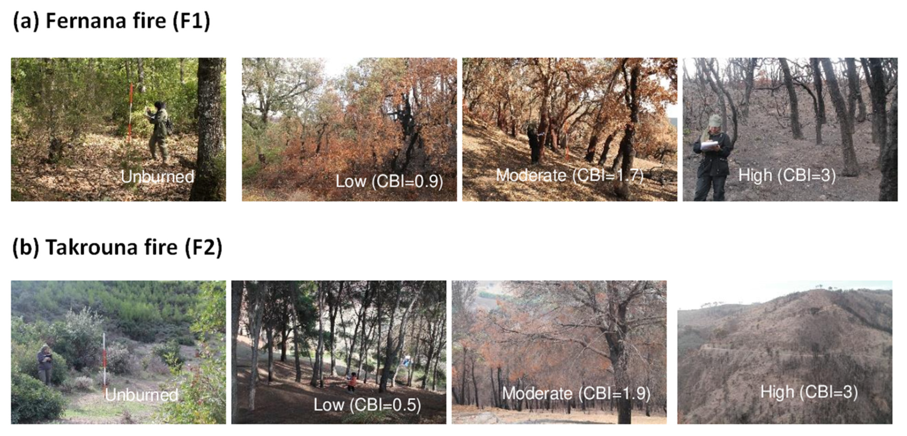
2.2.2. Field Data Collection

Between October and November 2021, field surveys were conducted to quantify fire severity on both fires (Table 3). Note that the time lag between CBI sampling and post-fire image acquisition is an important factor to consider in CBI modelling as it can be a major source of uncertainty, especially if field data were collected several weeks after the fire or if rapid ecosystem recovery is a concern [35]. In this study, we did not observe any regeneration process that can distort or hide the fire effects. A random sampling strategy was used with a circular plot of 15 m radius. A total of 193 plots were created, including 84 and 109 plots for the Fernana and Takrouna test areas, respectively. Digital photographs were taken of the center of each plot and geographic coordinates were recorded using a global navigation satellite system (GNSS) receiver. Following Key and Benson [18] and Fernández-García et al. [26], the field protocol to calculate the composite burn index (CBI) consisted of scoring several variables from 0 (not burned) to 3 (severely burned) in four layers: (i) substrate, (ii) vegetation with a height of <1 m, (iii) vegetation with a height between 1 and 5 m, and (iv) trees with a height of >5 m. The CBI was determined by combining the scores of each layer for each plot. The resulting CBI scores were categorized into four burn severity levels as follows [18]: unburned (CBI: 0–0.1); low severity (CBI: 0.1–1.24); moderate severity (CBI: 1.25–2.24); and high severity (CBI: 2.25–3).

2.2.3. Spectral Indices Computation and Forest Fires Delineation

The spectral indices used in this study were: the normalized burn ratio (NBR, [40]), its relativized version RBR [31], the burned area index for Sentinel-2 (BAIS2, [34]), and the thermal anomaly index (TAI, [32]). The indices were calculated for each pair of images before and after fire (Table 4). Following the calculation of the spectral indices, the extent of each fire was delineated by thresholding the RBR index based on the Otsu algorithm [41], which is one of the best thresholding methods commonly used for image segmentation [42]. The Otsu thresholding method aims to find the optimal threshold (t) by maximizing the between-class variance in the segmented image [42].

2.2.4. Statistical Models

We examined the correlation between the CBI data and the spectral indices using different classification and regression trees or CART. Here, both fires were merged to have enough sampling points (total n = 193) and make models more robust. Accordingly, we included the initial fire of the sampling points as a categorical variable in the models.
Classification and regression trees (CART) [43] refer to decision tree models that can be used for either classification or regression. The CART algorithm constitutes the core of important algorithms such as bagged decision trees, random forest and boosted regression trees. Here, the simplest decision trees (RPART) were created by using the “rpart” model of the “train” function in the R package “caret” [44]. The “rpart” algorithm iteratively divides the dataset into smaller homogeneous groups with a set of decision rules [43]. The objective of each split is to maximize the homogeneity (purity) of each group according to the response predictor. As an output, a tree diagram is produced, with branches defined by the splitting criteria for the predictor variables and a set of terminal nodes representing the mean response of the dependent variable (in this case, the CBI) [45]. The rpart approach first builds maximal trees and then uses the complexity parameter (cp) and v-fold cross-validation to adjust the tree to an optimal size [46]. In the cross-validation technique, the data are divided into 10 randomly selected blocks of similar size, and one block is allocated for testing the predictive performance of trees developed with the remaining dataset [43]. In this study, we determined the optimum tree size considering the following parameters: 10-fold cross-validation with a complexity parameter (cp) of 0.01 and a minimum of 5 cases (minsplit = 5) in each split.
More complex and accurate decision trees were bagged decision trees (Bagging) and boosted regression trees (BRT). Bagging for classification and regression trees is one of the first machine learning ensemble algorithms designed to enhance the accuracy of CART [47]. It uses bootstrapping to create an ensemble of predictions. Bootstrap aggregation algorithm (or bagging) is a machine learning method for fitting multiple prediction models from a training dataset and then combining them into an ensemble prediction [48]. The theoretical concept behind bagging is to aggregate the results of the predictions of different base learners to produce a more accurate result. By averaging the models, bagging helps to reduce variance and minimize overfitting. Here, we fitted bagging trees using the following parameters: 70% of bagging fraction, a complexity parameter (cp) or learning rate of 0.01, and a minimum of 5 cases in each split. The bagging trees were calculated using the bagging function of the package “ipred” in R [49].
The boosted regression trees (BRTs) integrate many regression tree models (RT) using the boosting technique to optimize prediction performance [50]. In BRT models, two important parameters must be set in advance, namely the tree complexity (tc) and the learning rate (lr); both parameters determine the number of trees required for optimal prediction. In our experiments, we fitted BRT models with varying values for lr (0.1, 0.01, and 0.001) and a range of tc (3–8 nodes). Our goal here is to identify the combination of parameters that yields the lowest prediction error [51]. After checking, the parameters giving the best results were: tree complexity: 3 nodes; learning rate: 0.01; 70% of bagging fraction, and a minimum of 5 cases in each split. The relative importance of each predictor was measured based on how often the predictor was selected for splitting the data and the gain to the model resulting from the selection [49]. According to [52], a predictor is considered important if its relative importance is >= 5%. In this study, we implemented BRT models using the R package “gbm” [53] and the R code of Elith et al. [50].
In addition to the tree-based regression models mentioned earlier, we also used the generalized additive models (GAMs) [52] to relate the spectral indices to the CBI data collected from in situ sampling. In GAMs, the relationship between explanatory variables (i.e., spectral severity indices) and response variables (i.e., CBI data) is captured through fitting response curves with smoothing functions. Depending on the complexity of the data, these functions can take many forms from polynomial and quadratic to complex thin-plate spline [53]. Herein, the GAM models were fitted with soft smoothing functions (k = 10) avoiding complex fitting and using the R package “mgcv” [53].
The evaluation of the performance of the different regression models was based on the training data (70% n = 135) and the test data (30% n = 58), which allowed us to assess our ability to explain the observed data and predict the omitted data, respectively. For each model, two parameters for model accuracy were derived: (i) the root mean square error (RMSE) and (ii) the corrected goodness of fit or adjusted R2 of the fitted values for the training and test data.

3. Results

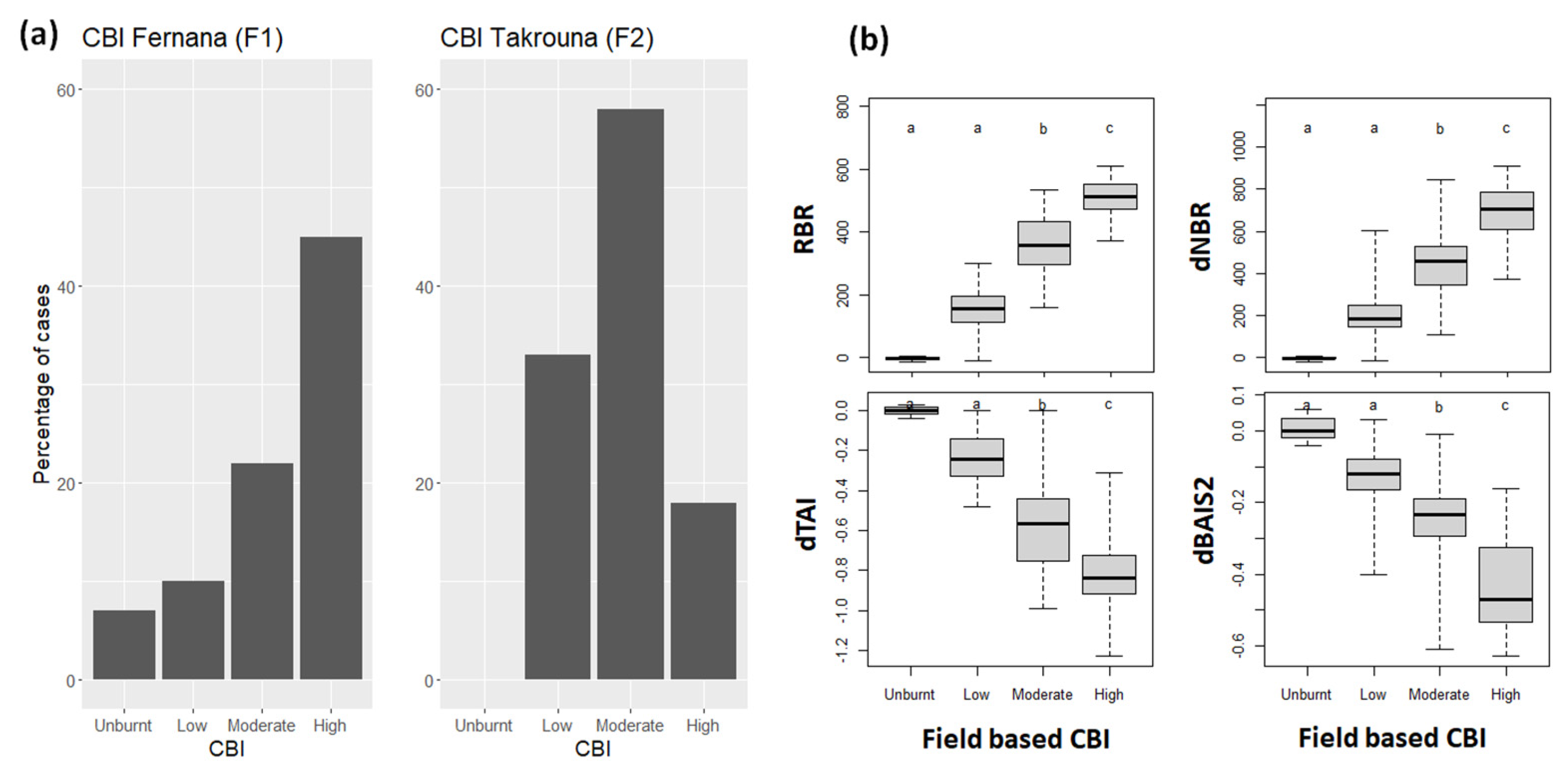
3.1. CBI Distribution

According to the CBI distribution on both fires, F1 (Fernana fire) burned under a higher intensity than F2 (Takrouna fire) (Figure 3a). In F1, 50% of the sampled points burned under high severity whereas in F2, only the 18% did, dominating the moderate conditions (58%). All the CBI classes, except unburned and low severity, were significantly different according to the spectral severity indices calculated (Figure 3b).

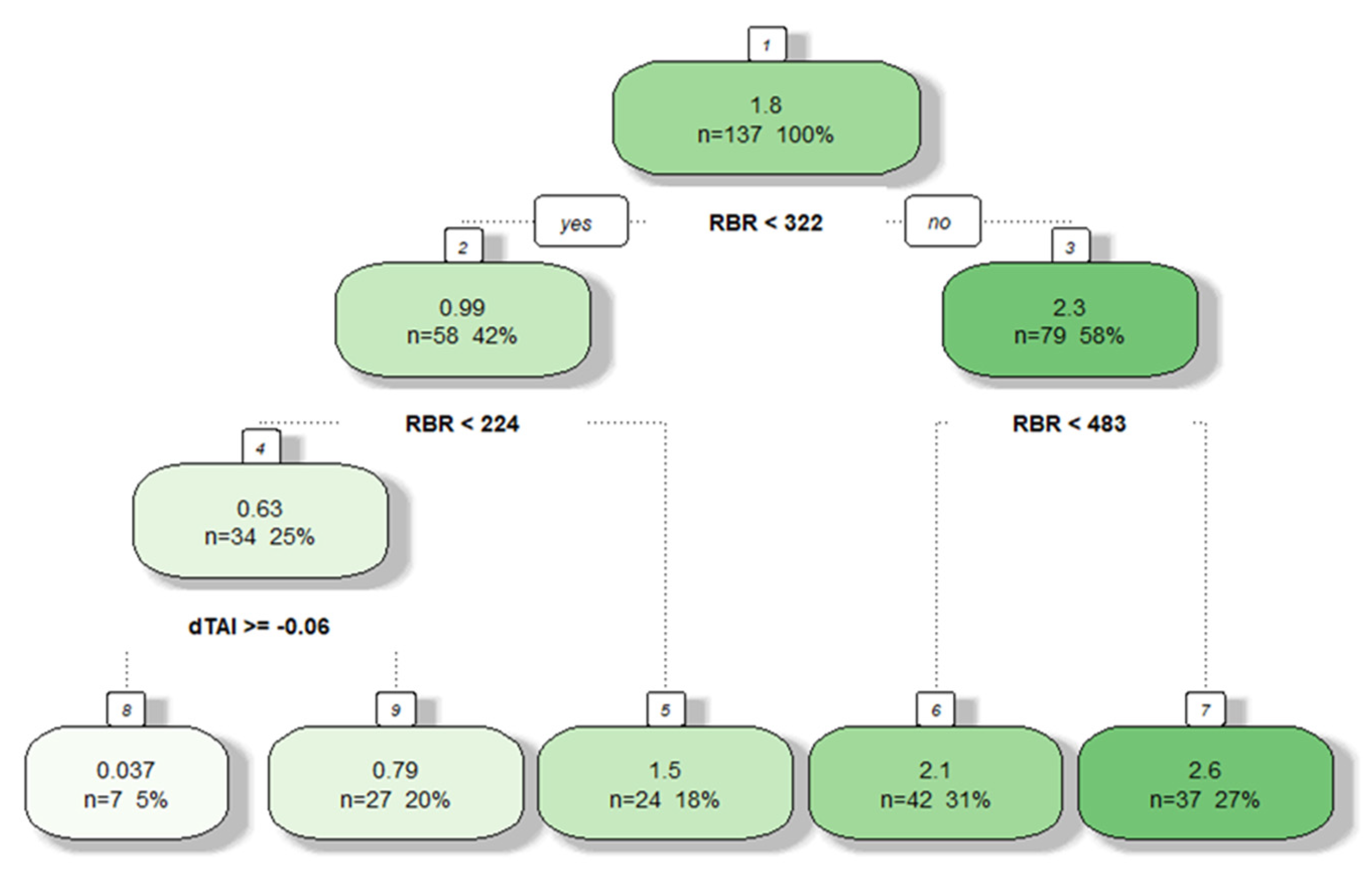
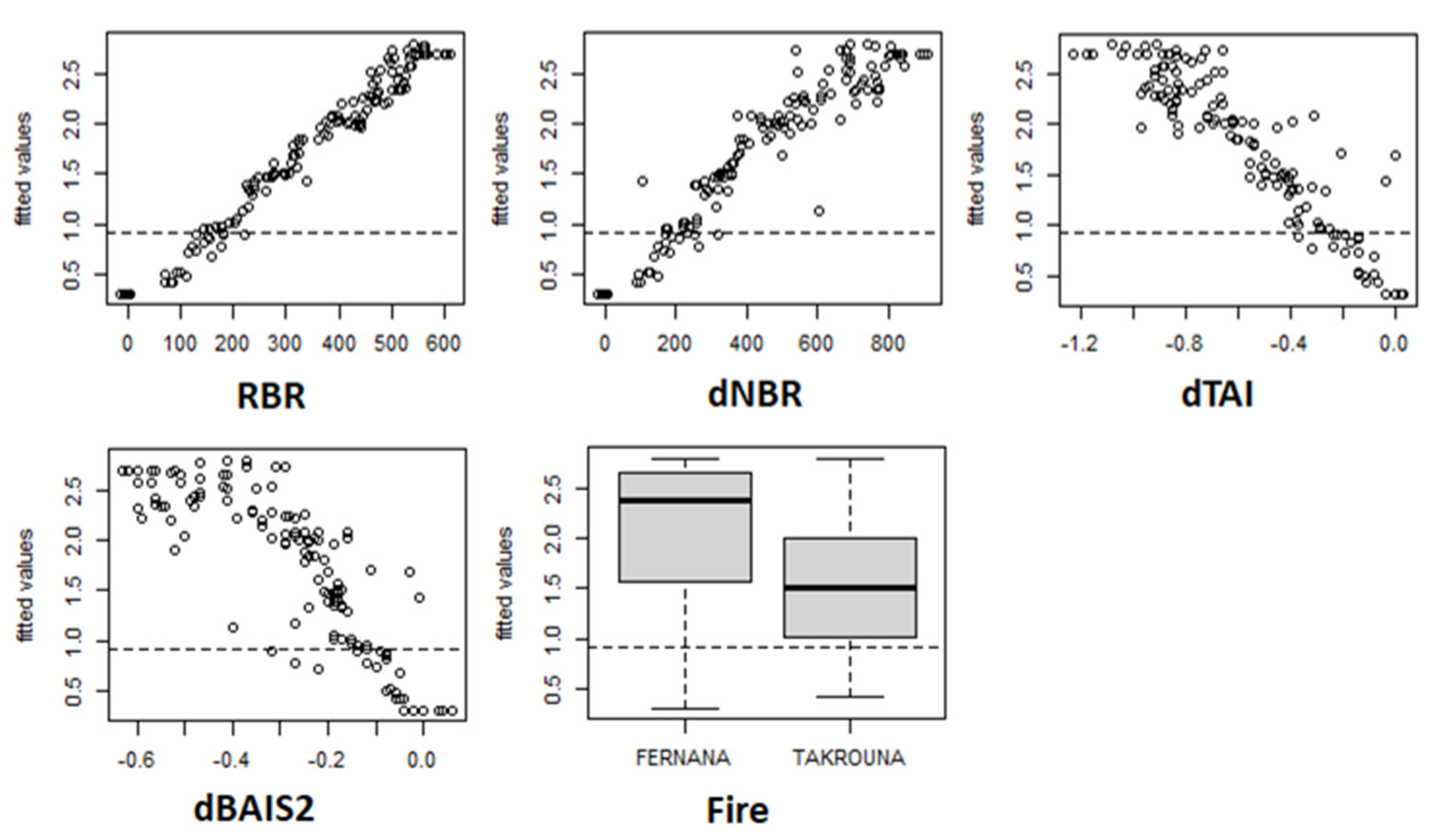
3.2. Models’ Predictions

The RPART model explained 88% and 87% of the CBI variance of training and test data, respectively with a root mean squared error (RMSE) less than 0.30 (Table 5 and Figure 4a). However, predictions were limited to 5 different values, because of the grouping effect of a single and short tree, which is one of the limitations of this approach. The main spectral index explaining the CBI was the RBR followed by dTAI (Figure 5a). Unburnt and low severity areas (CBI < 1.25) were characterized by low RBR (<223) values, areas burned under moderate severity by RBR values between 311–455, and high severity areas by RBR > 455 (Figure 6).
The bagging model explained more variance than RPART (Adj. R2 0.91 and 0.87, p < 0.001, for training and test data, respectively) (Table 5), and the points distribution in the scatterplot of observed versus predicted CBI values was better (Figure 4b). The spectral indices more important for explaining the CBI were the RBR followed by the dNBR. Both spectral indices gathered higher CBI variability than dTAI and dBAIS2 (Figure 5b).
On the other hand, the boosted regression trees (BRT) model explained more variance than RPART and bagging (Adj. R2 0.92 and 0.88, p < 0.001, for training and test data, respectively) (Table 5 and Figure 4c). The spectral indices more important for explaining the CBI were the RBR (65.5%) followed by the dNBR (25.9%) (Figure 5c). There was not any significant effect of the fire at which the sampling points belonged, although fire severity was slightly higher in F1 (Fernana) than in F2 (Takrouna) (Figure 7).
Finally, the generalized additive model (GAM) explained a similar variance to RPART (Adj. R2 0.88 and 0.85, p < 0.001, for training and test data, respectively), but showed higher error (Table 5 and Figure 4d). The spectral index more important for explaining the CBI was the RBR; dTAI was more significant than dNBR, and dBAIS2 was not significant (Figure 5d).

3.3. Spatialization of CBI Values from BRTs

The regression models between the observed field-based CBI and the predicted CBI values from the spatialized CBI using the BRT, indicated that fire severity in both fires was rather well predicted. In F1 (Fernana fire), the Adj. R2 was 0.82 with a RMSE of 0.37 and for F2 (Takrouna fire), the Adj.R2 was 0.76 and the RMSE of 0.34 (Figure 8). Moreover, the statistical distribution of the severity levels obtained in the maps of predicted CBI values matched quite well with the distribution of ground computed CBI (Figure 9). Nevertheless, in Takrouna fire, moderate severity (CBI: 1.25–2.24) was underestimated, increasing the proportion of low severity cases, whereas in Fernana fire, occurred the opposite, showing a slight overestimation of higher severity levels.

4. Discussion

The main findings of this study can be summarized as follows: (1) the most important spectral index explaining CBI was the RBR index, followed by dNBR; (2) the link between spectral severity indices and field-based CBI has a nonlinear character, and can be best fitted by the BRT model. The other three models show slightly less accurate predictive performance; and (3) although fire severity in F1 (Fernana) was slightly higher than in F2 (Takrouna), statistical analysis did not reveal any significant influence of the fire to which the sample points belonged. Each of these findings is discussed in more detail below.
There is considerable debate about which of the most-used spectral indices is appropriate for assessing burn severity, and under what conditions [54,55]. While some authors found a good correlation between NDVI and CBI data [56,57], the results suggest that NDVI is not sufficiently sensitive in sparsely vegetated and grassland areas [58,59,60]. Another limitation of NDVI for estimating fire severity is related to the saturation of this spectral index with high biomass values [61]. In contrast, spectral indices that include the SWIR band have shown stronger correlations with fire effects than NDVI [62,63]. The most appropriate NIR–SWIR index for estimating fire severity is the NBR [64]. This index has been used as a proxy to assess fire severity in a variety of biomes [16,22,65,66,67] becoming an operational index for estimating fire severity from satellite data. However, since fire severity depends on pre-fire vegetation conditions, Key and Benson [18] suggested using the difference between pre-fire and post-fire NBR values (dNBR).
Several studies have shown that the dNBR was the most appropriate spectral index for assessing and mapping forest fire severity [25,26,29,34,68,69]. However, it has also been demonstrated that dNBR can perform poorly as a predictor of CBI data in diverse environments with a heavy cover of shrubs and grasses [58,70]. In addition, dNBR has been shown to be strongly related to pre-fire vegetation; therefore, regions with low pre-fire green vegetation tend to display low dNBR values, regardless of fire severity [31]. For example, a pre-fire stand with 40% cover may have a moderate severity rating, while a stand with 70% cover may have a high severity rating. Epting et al. [63] found in interior Alaska that coniferous forests had higher fire severity (using dNBR) than deciduous forests and shrublands, and mean dNBR increased with increasing tree cover. The influence of pre-fire vegetation on dNBR is challenging in mixed forests, such as Mediterranean forests [71]. As an alternative, Miller and Thode [30] proposed a relative version of dNBR (RdNBR) that normalizes dNBR by the amount of pre-fire vegetation. According to Norton et al. [70], RdNBR provides greater accuracy of severity in grassland areas where low pre-fire total vegetation cover leads to relatively similar post-fire reflectivity. Since 2008, the National Forest System in California has adopted the RdNBR index as a standard for forest fire severity mapping. In this regard, good relationships have been observed between CBI and the RdNBR index [4,5,6,16,30,72]. Furthermore, in a California fire, De Santis et al. [36] found that the relationships between field severity data and RdNBR were higher (R2 = 0.68) than for dNBR, and that the variability of values dropped, particularly for high severity levels. Despite these advantages of RdNBR, the dispersion for moderate to low values was comparable to the results produced by dNBR. As Van Wagtendonk et al. [19] found, signal saturation was also noticeable for high severity levels when RdNBR was used. RBR is also a relativized version of dNBR, intended to counteract the tendency for RdNBR to lead to anomalous estimates of fire severity when pre-fire NBR is close to zero or negative [31]. Unlike the dNBR, the RBR index is less dependent on pre-fire vegetation cover and therefore can be used as a proxy for estimating fire severity across broad vegetation types and fire regimes [31,73]. A recent study by Gale et al. [72] showed a substantial difference in correlation between pre-fire NBR and dNBR (r = 0.23) and between pre-fire NBR and RBR (r = −0.03). This suggests that pre-fire NBR has a significant impact on the resulting dNBR index values, as it is a good indicator of pre-fire photosynthetic biomass as well as soil and leaf moisture [74]. Therefore, it is not surprising that in this study the RBR index has a higher performance in predicting CBI compared to the dNBR index. Our study confirms the findings of [6,31], who recommend the use of the RBR index over the dNBR index even when pre-fire vegetation cover is sparse. Such forested areas are very common in Tunisia and are likely to become more common due to climate change. In contrast, RBR may not provide an improvement over dNBR if pre-fire vegetation cover is spatially continuous.
Conversely, the performance of BAIS2 in this study was surprisingly lower than expected, considering the high efficiency reported by [34,75] in forest-fire mapping. This index takes advantage of the broader spectrum of the Sentinel 2 bands in the visible, red edge, NIR, and SWIR areas, which theoretically would have a better correlation with the CBI field data. However, according to our findings, the index does not seem to be suitable for predicting fire severity. Our findings support those of Holden et al. [8], who reported similar weak performance of BAIS2 in assessing fire severity compared to conventional spectral severity indices such as dNBR and RBR.
Similarly to BAIS2, the TAI showed a relatively low correlation with the CBI data compared to dNBR and RBR. This index was recently developed to detect fire anomalies (industrial heat sources) from Sentinel 2 imagery [32] and was used in this study to test its efficiency in predicting fire severity. However, as far as we know, this is the first study to use the TAI index to predict fire severity. Therefore, further research should be conducted to confirm or refute our findings. Finally, as indicated by Lentile et al. [16] in most studies assessing the degree of severity with standard indices of Landsat TM data (e.g., NBR, dNBR or RdNBR), thermal infrared is not used, even though it can provide very useful information on the exposed soils due to vegetation removal.
Four regression models (i.e., RPART, bagging, BRT, and GAM) were used in the study to estimate the predictive power of several severity spectral indices in fitting field-based CBI. The best relationship was obtained by the BRT model with the highest R2 (Adj. R2: 0.92 for training data) and the smallest RMSE. The RPART, bagging, and GAM algorithms also displayed a positive correlation, but with lower R2 and higher values of RMSE. The main disadvantage of RPART relied on categorizing continuous predictors at the time of node splitting, losing some of their information. The performance achieved with BRT supports recent literature showing a similar performance of this model in predicting fire severity [6] and better performance than other published machine learning models [38,76], but lower than that of Boucher et al. [77], who reported an Adj.R2 of 0.93 using the GAM model. Parks et al. [78], for example, examined the correlation between RBR and CBI data collected from 263 fires in the United States and Canada using a random forest (RF) model and reported an Adj.R² of 0.72. Similarly, Kurbanov et al. [66] used four regression models to estimate the relationship between field-based CBI and dNBR. Their results showed that the third-degree polynomial model was the best regression model with the highest R2 of 0.79. Furthermore, Zheng et al. [39] used a support vector regression (SVR) and regression analysis method (RA) to predict CBI values as a function of dNBR. The results show that the performance of SVR is more accurate (RMSE = 0.46–0.57) than that of RA (RMSE = 0.53–0.68). Taken together, these studies and our results confirm the non-linear relationship between CBI data and spectral severity indices. Being able to estimate with precision the risk of large wildfires, as well as their severity, is crucial for the agencies responsible for the prevention and extinction of wildfires. Understanding post-fire effects (severity) and fire behavior will contribute to the development of better tools for assessing and predicting the effects of fires on forest ecosystems, as well as predicting when and where a forest fire is more likely to cause major damage.

5. Conclusions

The present study was designed to predict the severity of forest fires in Tunisia by relating several spectral severity indices to CBI data collected from in situ sampling plots using different regression methods. Several findings emerge from this study. First, the RBR index was the best predictor of field-based CBI for both fires, regardless of the regression model used. Out of the four regression models tested in this study, the BRT model displayed the best performance in terms of accuracy metrics, although the difference between all models was not too pronounced. From these results, we can conclude that the RBR-based BRT model with better accuracy performance should be recommended for future research on mapping wildfire severity at least in northern Tunisia. This is an important finding, because it is not a feasible task to collect field data and build a model for every fire. However, these results may not be generalizable to other regions or consistent, at least, at the national level, given the small number of fire events investigated in this study. Further research needs to examine in more detail the relationships between spectral severity indices and CBI data for other biomes that experience a range of fire types (from surface to crown fires) and fire regimes in terms of frequency and intensity before the results of the current study can be generalized. Finally, this study highlights the importance of incorporating spectral indices and field data, and exploring non-parametric models, including machine learning algorithms, to accurately predict fire severity.

Author Contributions

All authors contributed to the study conception and design. Material preparation, data collection and analysis were performed by M.A., H.A. and O.V. The first draft of the manuscript was written by M.A., O.V. and H.A. And the study was supervised by C.A., O.V. and H.A. All authors have read and agreed to the published version of the manuscript.

Funding

This research is part of the project INFORICAM (PID2020-119402RB-I00), funded by the Spanish MCIN/AEI/10.13039/501100011033 and by the “European Union NextGenerationEU/PRTR”.

Data Availability Statement

The data that support the findings of this study are available from the corresponding author, upon reasonable request.

Acknowledgments

This research acknowledges the funding received from the INFORICAM project (PID2020-119402RB-I00). The authors would like to thank Jose Manuel Moreno Rodriguez for his useful comments and help.

Conflicts of Interest

The authors declare no conflict of interest.

References

  1. Miller, J.D.; Safford, H.D.; Crimmins, M.; Thode, A.E. Quantitative evidence for increasing forest fire severity in the Sierra Nevada and southern Cascade Mountains, California and Nevada, USA. Ecosystems 2009, 12, 16–32. [Google Scholar] [CrossRef]
  2. Mueller, V.; Gray, C.; Hopping, D. Climate-Induced migration and unemployment in middle income Africa. Glob. Environ. Chang. 2020, 65, 102183. [Google Scholar] [CrossRef] [PubMed]
  3. Parks, S.A.; Abatzoglou, J.T. Warmer and Drier Fire Seasons Contribute to Increases in Area Burned at High Severity in Western US Forests From 1985 to 2017. Geophys. Res. Lett. 2020, 47, e2020GL089858. [Google Scholar] [CrossRef]
  4. French, N.H.F.; Kasischke, E.S.; Hall, R.J.; Murphy, K.A.; Verbyla, D.L.; Hoy, E.E.; Allen, J.L. Using Landsat data to assess fire and burn severity in the North American boreal forest region: An overview and summary of results. Int. J. Wildl. Fire 2008, 17, 443–462. [Google Scholar] [CrossRef]
  5. Viedma, O.; Quesada, J.; Torres, I.; De Santis, A.; Moreno, J.M. Fire severity in a large fire in a Pinus pinaster forest is highly predictable from burning conditions, stand structure, and topography. Ecosystems 2015, 18, 237–250. [Google Scholar] [CrossRef]
  6. Viedma, O.; Chico, F.; Fernández, J.J.; Madrigal, C.; Safford, H.D.; Moreno, J.M. Disentangling the role of prefire vegetation vs. burning conditions on fire severity in a large forest fire in SE Spain. Remote Sens. Environ. 2020, 247, 111891. [Google Scholar] [CrossRef]
  7. Doerr, S.H.; Shakesby, R.A.; Blake, W.H.; Chafer, C.J.; Humphreys, G.S.; Wallbrink, P.J. Effects of differing wildfire severities on soil wettability and implications for hydrological response. J. Hydrol. 2006, 319, 295–311. [Google Scholar] [CrossRef]
  8. Holden, Z.A.; Morgan, P.; Evans, J.S. A predictive model of burn severity based on 20-year satellite-inferred burn severity data in a large southwestern US wilderness area. For. Ecol. Manag. 2009, 258, 2399–2406. [Google Scholar] [CrossRef]
  9. Miller, J.E.D.; Root, H.T.; Safford, H.D. Altered fire regimes cause long-term lichen diversity losses. Glob. Chang. Biol. 2018, 24, 4909–4918. [Google Scholar] [CrossRef]
  10. Keeley, J.E.; Brennan, T.; Pfaff, A.H. Fire severity and ecosystem responses following crown fires in California shrublands. Ecol. Appl. 2008, 18, 1530–1546. [Google Scholar] [CrossRef] [PubMed]
  11. Van der Werf, G.R.; Randerson, J.T.; Giglio, L.; Collatz, G.J.; Kasibhatla, P.S.; Arellano, A.F., Jr. Interannual variability in global biomass burning emissions from 1997 to 2004. Atmos. Chem. Phys. 2006, 6, 3423–3441. [Google Scholar] [CrossRef] [Green Version]
  12. Alonzo, M.; Morton, C.D.; Cook, D.B.; Andersen, H.E.; Babcock, C.; Pattison, R. Patterns of canopy and surface layer consumption in a boreal forest fire from repeat airborne lidar. Environ. Res. Lett. 2017, 12, 065004. [Google Scholar] [CrossRef]
  13. Keeley, J.E. Fire intensity, fire severity and burn severity: A brief review and suggested usage. Int. J. Wildland Fire 2009, 18, 116–126. [Google Scholar] [CrossRef]
  14. Morgan, P.; Keane, R.E.; Dillon, G.K.; Jain, T.B.; Hudak, A.T.; Karau, E.C.; Sikkink, P.G.; Holden, Z.A.; Strand, E.K. Challenges of assessing fire and burn severity using field measures, remote sensing and modelling. Int. J. Wildland Fire 2014, 23, 1045. [Google Scholar] [CrossRef] [Green Version]
  15. Stow, D.; Fulé, P.Z.; Crouse, J.E. Comparison of burn severity assessments using Differenced Normalized Burn Ratio and ground data. Int. J. Wildland Fire 2005, 14, 189–198. [Google Scholar]
  16. Lentile, L.B.; Holden, Z.A.; Smith, A.M.S.; Falkowski, M.J.; Hudak, A.T.; Morgan, P.; Lewis, S.A.; Gessler, P.E.; Benson, N.C. Remote sensing techniques to assess active fire and post-fire effects. Int. J. Wildland Fire 2006, 15, 319–345. [Google Scholar] [CrossRef]
  17. Moreno, J.M.; Torres, I.; Luna, B.; Oechel, W.C.; Keeley, J.E. Changes in fire intensity have carry-over effects on plant responses after the next fire in southern California chaparral. J. Veg. Sci. 2013, 24, 395–404. [Google Scholar] [CrossRef] [Green Version]
  18. Key, C.H.; Benson, N.C. Landscape Assessment (LA): Sampling and Analysis Methods; USDA Forest Service, Rocky Mountain Research Station: Fort Collins, CO, USA, 2006; pp. 1–55. [Google Scholar] [CrossRef]
  19. Van Wagtendonk, J.W.; Root, R.R.; Key, C.H. Comparison of AVIRIS and Landsat ETM+ detection capabilities for burn severity. Remote Sens. Environ. 2004, 92, 397–408. [Google Scholar] [CrossRef]
  20. Cansler, C.A.; McKenzie, D. How Robust Are Burn Severity Indices When Applied in a New Region? Evaluation of Alternate Field-Based and Remote-Sensing Methods. Remote Sens. 2012, 4, 456–483. [Google Scholar] [CrossRef] [Green Version]
  21. Fassnacht, F.E.; Schmidt-Riese, E.; Kattenborn, T.; Hernandez, J. Explaining Sentinel 2-based dNBR and RdNBR variability with reference data from the bird’s eye (UAS) perspective. Int. J. Appl. Earth. Obs. Geoinf. 2021, 95, 102262. [Google Scholar] [CrossRef]
  22. De Santis, A.; Chuvieco, E. GeoCBI: A Modified Version of the Composite Burn Index for the Initial Assessment of the Short-Term Burn Severity from Remotely Sensed Data. Remote Sens. Environ. 2009, 113, 554–562. [Google Scholar] [CrossRef]
  23. Gallagher, M.R.; Skowronski, N.S.; Lathrop, R.G.; McWilliams, T.; Green, E.G. An Improved Approach for Selecting and Validating Burn Severity Indices in Forested Landscapes. Can. J. Remote Sens. 2020, 46, 100–111. [Google Scholar] [CrossRef]
  24. Eva, H.; Lambin, E.F. Remote Sensing of Biomass Burning in Tropical Regions: Sampling Issues and Multisensor Approach. Remote Sens. Environ. 1998, 64, 292–315. [Google Scholar] [CrossRef]
  25. Mallini, G.; Mitsopoulos, I.; Chrysafi, I. Evaluating and comparing sentinel 2A and Landsat-8 operational land imager (OLI) spectral indices for estimating fire severity in a mediterranean pine ecosystem of Greece. GIsci. Remote Sens. 2017, 55, 1–18. [Google Scholar] [CrossRef]
  26. Fernández-García, V.; Santamartaa, M.; Fernández-Manso, A.; Quintano, C.; Marcos, E.; Calvo, L. Burn severity metrics in fire-prone pine ecosystems along a climatic gradient using Landsat imagery. Remote Sens. Environ. 2018, 206, 205–217. [Google Scholar] [CrossRef]
  27. Garcıa-Llamas, P.; Suarez-Seoane, S.; Fernandez-Manso, A.; Quintano, C.; Calvo, L. Evaluation of fire severity in fire prone ecosystems of Spain under two different environmental conditions. J. Environ. Manag. 2020, 271, 110706. [Google Scholar] [CrossRef]
  28. Collins, L.; McCarthy, G.; Mellor, A.; Newell, G.; Smith, L. Training data requirements for fire severity mapping using Landsat imagery and random forest. Remote Sens. Environ. 2020, 245, 111839. [Google Scholar] [CrossRef]
  29. Gibsona, R.; Danahera, T.; Hehirc, W.; Collins, L. A remote sensing approach to mapping fire severity in south-eastern Australia using sentinel 2 and random forest. Remote Sens. Environ. 2020, 240, 111702. [Google Scholar] [CrossRef]
  30. Miller, J.D.; Thode, A.E. Quantifying burn severity in a heterogeneous landscape with a relative version of the delta normalized burn ratio (dNBR). Remote Sens. Environ. 2007, 109, 66–80. [Google Scholar] [CrossRef]
  31. Parks, S.A.; Dillon, G.K.; Miller, C. A new metric for quantifying burn severity: The relativized burn ratio. Remote Sens. 2014, 6, 1827–1844. [Google Scholar] [CrossRef]
  32. Liu, Y.; Zhi, W.; Xu, B.; Xu, W.; Wu, W. Detecting high-temperature anomalies from Sentinel-2 MSI images. ISPRS J. Photogramm. Remote Sens. 2021, 177, 174–193. [Google Scholar] [CrossRef]
  33. Achour, H.; Toujani, A.; Trabelsi, H.; Jaouadi, W. Evaluation and comparison of Sentinel-2 MSI, Landsat 8 OLI, and EFFIS data for forest fires mapping. Illustrations from the summer 2017 fires in Tunisia. Geocarto Int. 2021, 37, 7021–7040. [Google Scholar] [CrossRef]
  34. Filipponi, F. BAIS2: Burned area index for Sentinel-2. Proceedings 2018, 2, 364. [Google Scholar]
  35. Veraverbeke, S.; Verstraeten, W.; Lhermite, S.; Goossens, R. Evaluating Landsat thematic mapper spectral indices for estimating burn severity of the 2007 Peloponnese wildfires in Greece. Int. J. Wildland Fire 2010, 19, 558–569. [Google Scholar] [CrossRef] [Green Version]
  36. De Santis, A.; Asner, G.P.; Vaughan, P.J.; Knapp, E.D. Mapping burn severity and burning efficiency in California using simulation models and Landsat imagery. Remote Sens. Environ. 2010, 114, 1535–1545. [Google Scholar] [CrossRef]
  37. Picotte, J.J.; Robertson, K.M. Validation of remote sensing of burn severity in south-eastern US ecosystems. Int. J. Wildland Fire 2011, 20, 453–464. [Google Scholar] [CrossRef]
  38. Garcıa-Llamas, P.; Suarez-Seoane, S.; Fernandez-Guisuraga, J.M.; Fernandez-Garcıa, V.; Fernandez-Manso, A.; Quintano, C.; Taboada, A.; Marcos, E.; Calvo, L. Evaluation and comparison of Landsat 8, Sentinel-2 and Deimos-1 remote sensing indices for assessing burn severity in Mediterranean fire prone ecosystems. Int. J. Appl. Earth. Obs. Geoinf. 2019, 80, 137–144. [Google Scholar] [CrossRef]
  39. Zheng, Z.; Zeng, Y.; Li, S.; Huang, W. Mapping Burn Severity of Forest Fires in Small Sample Size Scenarios. Forests 2018, 9, 608. [Google Scholar] [CrossRef] [Green Version]
  40. Key, C.; Benson, N. Landscape assessment: Ground measure of severity, the composite burn index, and remote sensing of severity, the normalized burn index. In FIREMON: Fire Effects Monitoring and Inventory System; General Technical Report RMRS-GTR-164-CD LA; Lutes, D., Keane, R., Caratti, J., Key, C., Benson, N., Sutherland, S., Gangi, L., Eds.; USDA Forest Service, Rocky Mountains Research Station: Fort Collins, CO, USA, 2005; pp. 1–51. [Google Scholar]
  41. Otsu, N. A Threshold Selection Method from Gray-Level Histograms. IEEE Trans. Syst. Man Cybern. 1979, 9, 62–6642. [Google Scholar] [CrossRef] [Green Version]
  42. Munoz-Minjares, J.; Vite-Chavez, O.; Flores-Troncoso, J.; Cruz-Duarte, J.M. Alternative Thresholding Technique for Image Segmentation Based on Cuckoo Search and Generalized Gaussians. Mathematics 2021, 9, 2287. [Google Scholar] [CrossRef]
  43. Breiman, L.; Friedman, J.; Stone, C.J.; Olshen, R.A. Classification and Regression Trees. Biom. J. 1984, 40, 874. [Google Scholar]
  44. Kuhn, M. Building Predictive Models in R Using the caret Package. J. Stat. Softw. 2008, 28, 1–26. [Google Scholar] [CrossRef]
  45. Viedma, O.; Torres, I.; Pérez, B.; Moreno, J.M. Modeling plant species richness using reflectance and texture data derived from QuickBird in a recently burned area of Central Spain. Remote. Sens. Environ. 2012, 119, 208–221. [Google Scholar] [CrossRef]
  46. De’ath, G.; Fabricius, K.E. Classification and regression trees: A powerful yet simple technique for ecological data analysis. Ecology 2000, 81, 3178–3192. [Google Scholar] [CrossRef]
  47. Breiman, L. Arcing Classifiers. Ann. Stat. 1998, 26, 801–849. [Google Scholar]
  48. Breiman, L. Bagging Predictors. Mach Learn. 1996, 24, 123–140. [Google Scholar] [CrossRef] [Green Version]
  49. Peters, A.; Hothorn, T. Ipred: Improved Predictors, Version 0.9–3. R Package. 2013. Available online: http://CRAN.R-project.org/package=ipred (accessed on 20 February 2022).
  50. Elith, J.; Leathwick, J.R.; Hastie, T. A working guide to boosted regression trees. J. Anim. Ecol. 2008, 77, 802–813. [Google Scholar] [CrossRef]
  51. Knudby, A.; Newman, C.; Shaghude, Y.; Muhando, C. Simple and effective monitoring of historic changes in nearshore environments using the free archive of Landsat imagery. Int. J. Appl. Earth. Obs Geoinf. 2010, 12S, S116–S122. [Google Scholar] [CrossRef]
  52. Le Parisien, M.A.; Parks, S.A.; Krawchuk, M.A.; Flannigan, M.D.; Bowman, L.M.; Moritz, M.A. Scale dependent controls on the area burned in the boreal forest of Canada, 1980–2005. Ecol Appl. 2011, 21, 789–805. [Google Scholar] [CrossRef] [Green Version]
  53. Ridgeway, G. Generalized Boosted Models: A Guide to the Gbm Package; 2007. Available online: https://cran.r-project.org/web/packages/gbm/vignettes/gbm.pdf (accessed on 1 November 2022).
  54. Parks, S.A.; Holsinger, L.M.; Panunto, M.H.; Jolly, W.M.; Dobrowski, S.Z.; Dillon, G.K. High severity fire: Evaluating its key drivers and mapping its probability across western US forests. Environ. Res. Lett. 2018, 13, 044037. [Google Scholar] [CrossRef]
  55. Harvey, B.J.; Andrus, R.A.; Anderson, S.C. Incorporating biophysical gradients and uncertainty into burn severity maps in a temperate fire-prone forested region. Ecosphere 2019, 10, e02600. [Google Scholar] [CrossRef] [Green Version]
  56. Chafer, C.J.; Noonan, M.; Macnaught, E. The post-fire measurement of fire severity and intensity in the Christmas 2001 Sydney wildfires. Int. J. Wildland Fire 2004, 13, 227–240. [Google Scholar] [CrossRef]
  57. Hammill, K.A.; Bradstock, R.A. Remote sensing of fire severity in the Blue Mountains: Influence of vegetation type and inferring fire intensity. Int. J. Wildland Fire 2006, 15, 213–226. [Google Scholar] [CrossRef]
  58. Rogan, J.; Yool, S.R. Mapping fire-induced vegetation depletion in the Peloncillo Mountains: Arizona and New Mexico. Int. J. Remote. Sens. 2001, 22, 3101–3121. [Google Scholar] [CrossRef]
  59. Epting, J.; Verbyla, D.; Sorbel, B. Evaluation of Remotely Sensed Indices for Assessing Burn Severity in Interior Alaska Using Landsat TM and ETM+. Remote Sens. Environ. 2005, 96, 328–339. [Google Scholar] [CrossRef]
  60. Chuvieco, E.; Riaño, D.; Danson, F.M.; Martin, P. Use of a radiative transfer model to simulate the postfire spectral response to burn severity. J. Geophys. Res. 2006, 111, G04S09. [Google Scholar] [CrossRef] [Green Version]
  61. Key, C.H.; Benson, N.C. Fire Effects Monitoring and Inventory Protocol—Landscape Assessment; USDA Forest Service Fire Science Laboratory: Missoula, MT, USA, 2002. [Google Scholar]
  62. Miller, J.D.; Yool, S.R. Mapping Forest post-fire canopy consumption in several overstory types using multi-temporal Landsat TM and ETM data. Remote Sens. Environ. 2002, 82, 481–496. [Google Scholar] [CrossRef]
  63. Smith, A.M.S.; Wooster, M.J.; Drake, N.A.; Dipotso, F.M.; Falkowski, M.J.; Hudak, A.T. Testing the potential of multispectral remote sensing for retrospectively estimating fire severity in African savanna environments. Remote Sens. Environ. 2005, 97, 92–115. [Google Scholar] [CrossRef] [Green Version]
  64. Stow, D.; Lopez, A.; Lippitt, C.; Hinton, S.; Weeks, J. Object-based classification of residential land use within Accra, Ghana based on QuickBird satellite data. Int. J. Remote Sens. 2007, 28, 5167–5173. [Google Scholar] [CrossRef] [Green Version]
  65. De Santis, A.; Chuvieco, E. Burn severity estimation from remotely sensed data: Performance of simulation versus empirical models. Remote Sens. Environ. 2007, 108, 422–435. [Google Scholar] [CrossRef]
  66. Kurbanov, E.; Vorobyev, O.; Leznin, S.; Polevshikova, Y.; Demisheva, E. Assessment of burn severity in Middle Povozhje with Landsat multitemporal data. Int. J. Wildland Fire 2017, 26, 772–782. [Google Scholar] [CrossRef]
  67. Martini, L.; Faes, L.; Picco, L.; Iroumé, A.; Lingua, E.; Garbarino, M.; Cavalli, M. Assessing the effect of fire severity on sediment connectivity in central Chile. Sci. Total Environ. 2020, 728, 139006. [Google Scholar] [CrossRef] [PubMed]
  68. Allen, J.L.; Sorbel, B. Assessing the differenced normalized burn Ratio’s ability to map burn severity in the boreal forest and tundra ecosystems of Alaska’s national parks. Int. J. Wildland Fire 2008, 17, 463–475. [Google Scholar] [CrossRef]
  69. Safford, H.D.; Betancourt, J.L.; Hayward, G.D.; Wiens, J.A.; Regan, C.A. Land management in the Anthropocene: Is history still relevant? Eos 2008, 89, 343. [Google Scholar] [CrossRef] [Green Version]
  70. Norton, J.; Glenn, N.; Germino, M.; Weber, K.; Seefeldt, S. Relative suitability of indices derived from Landsat ETM+ and SPOT 5 for detecting fire severity in sagebrush steppe. Int. J. Appl. Earth. Obs. Geoinf. 2009, 11, 360–367. [Google Scholar] [CrossRef]
  71. Stambaugh, M.C.; Varner, J.M.; Noss, R.F.; Dey, D.C.; Christensen, N.L.; Baldwin, R.F.; Guyette, R.P.; Hanberry, B.B.; Harper, C.A.; Lindblom, S.G.; et al. Clarifying the role of fire in the deciduous forests of eastern North America: Reply to Matlack. Conserv. Biol. 2015, 29, 942–946. [Google Scholar] [CrossRef]
  72. Gale, M.G.; Cary, G.J. What determines variation in remotely sensed fire severity? Consideration of remote sensing limitations and confounding factors. Int. J. Wildland Fire 2022, 31, 291–305. [Google Scholar] [CrossRef]
  73. Silva-Cardoza, A.I.; Vega-Nieva, D.J.; Briseño-Reyes, J.; Briones-Herrera, C.I.; López-Serrano, P.M.; Corral-Rivas, J.J.; Parks, A.S.; Holsinger, M.L. Evaluating a New Relative Phenological Correction and the Effect of Sentinel-Based Earth Engine Compositing Approaches to Map Fire Severity and Burned Area. Remote Sens. 2022, 14, 3122. [Google Scholar] [CrossRef]
  74. Chuvieco, E.; Aguado, I.; Salas, J.; García, M.; Yebra, M.; Oliva, P. Satellite Remote Sensing Contributions to Wildland Fire Science and Management. Curr. Forestry Rep. 2020, 6, 81–96. [Google Scholar]
  75. Smiraglia, D.; Filipponi, F.; Mandrone, S.; Tornato, A.; Taramelli, A. Agreement Index for Burned Area Mapping: Integration of Multiple Spectral Indices Using Sentinel-2 Satellite Images. Remote Sens. 2020, 12, 1862. [Google Scholar] [CrossRef]
  76. Smith, C.W.; Panda, S.K.; Bhatt, U.S.; Meyer, F.J.; Badola, A.; Hrobak, L.J. Assessing Wildfire Burn Severity and Its Relationship with Environmental Factors: A Case Study in Interior Alaska Boreal Forest. Remote Sens. 2021, 3, 1966. [Google Scholar] [CrossRef]
  77. Boucher, J.; Beaudoin, A.; Hébert, C.; Guindon, L.; Bauce, E. Assessing the potential of the differenced Normalized Burn Ratio (dNBR) for estimating burn severity in eastern Canadian boreal forests. Int. J. Wildland Fire 2016, 26, 32–45. [Google Scholar] [CrossRef]
  78. Parks, S.A.; Holsinger, L.M.; Koontz, M.J.; Collins, L.; Whitman, E.; Parisien, M.A.; Loehman, R.A.; Barnes, J.L.; Bourdon, J.F.; Boucher, J.; et al. Giving Ecological Meaning to Satellite-Derived Fire Severity Metrics across North American Forests. Remote Sens. 2019, 11, 1735. [Google Scholar] [CrossRef]
Figure 1. Location of the selected fires in Tunisia. Sentinel 2A false color images (red: band 12, green: band 8, blue: band 4) depicting the Fernana (F1) and Takrouna (F2) fire scars. The extent of each fire (black contour polygons in the bottom panels) was delineated by thresholding the RBR index.
Remotesensing 15 00335 g001
Figure 2. Field photos showing the different levels of severity assigned in the Fernana (a) and Takrouna fires (b).
Remotesensing 15 00335 g002
Figure 3. (a) Percentage of occupation of the different CBI classes using the entire data set (n = 193): unburnt (CBI: 0–0.1), low severity (CBI: 0.1–1.24), moderate severity (CBI: 1.25–2.24), and high severity (CBI: 2.25–3) for both fires of Fernana (F1) and Takrouna (F2); and (b) boxplots of the different spectral severity indices in each CBI class merging both fires. Letters indicated the separability among CBI classes according to the post-hoc Kruskal-Wallis Dunn test.
Remotesensing 15 00335 g003
Figure 4. Scatterplots between predicted and observed CBI values merging both fires (Fernana and Takrouna) and using only test data (n = 58) from: (a) the regression tree (RPART); (b) the bagging, (c) the boosted regression tree (BRT), and (d) generalized additive (GAM) models.
Remotesensing 15 00335 g004
Figure 5. Partial dependence of CBI on the spectral severity indices used as explanatory variables from: (a) the regression tree (RPART); (b) the bagging; (c) the boosted regression tree (BRT); and (d) generalized additive (GAM) models using training data (n = 135). Here, it is shown only the significant spectral severity indices (RBR, dNBR, and dTAI).
Remotesensing 15 00335 g005
Figure 6. Regression tree (RPART) model for explaining CBI based on spectral severity indices (RBR, dNBR, dTAI, and dBAIS2) used as explanatory variables.
Remotesensing 15 00335 g006
Figure 7. Raw correlations between the CBI and the spectral severity indices (RBR, dNBR, dTAI, and dBAIS2) and the fire at which the sampling points belonged in the boosted regression trees (BRT).
Remotesensing 15 00335 g007
Figure 8. Maps of predicted CBI values derived from the boosted regression trees (BRT) in both fires analyzed: (top) F1 (Fernana fire) and (bottom) F2 (Takrouna fire). Inset are shown the scatterplot between the field-observed and spatialized predicted CBI values using BRT.
Remotesensing 15 00335 g008
Figure 9. (a) Percentage of occupation of the predicted CBI classes from the spatialized CBI using the BRT: unburnt (CBI: 0–0.1), low severity (CBI: 0.1–1.24), moderate severity (CBI: 1.25–2.24), and high severity (CBI: 2.25–3) for both fires of Fernana (F1) and Takrouna (F2); and (b) boxplots of the different spectral severity indices in each CBI class merging both fires. Letters indicate the separability among CBI classes according to the post-hoc Kruskal–Wallis Dunn test.
Remotesensing 15 00335 g009
Table 1. Locations, ignition dates and extent of forest fires considered in this study.
Ignition DateDurationArea (ha)Locality
F1 11 August 20212 days1500Fernana/Jendouba
F2 25 July 20214 days3000Takrouna/Sakiet sidi Youssef/Kef
Table 2. Some characteristics of the Sentinel 2 images used in this study.
EventAcquisition
Date
Acquisition
Time
SensorSun Zenith
Angle (°)
Solar Azimuth Angle (°)
L1C_T32SMF_A031908_20210801T102027Prefire F101 August 202110:20:27.348ZS2A24135
L1C_T32SMF_A031622_20210712T101027Prefire F212 July 202112:26:47.000ZS2A21129
L1C_T32SMF_A032194_20210821T102026Post-fire F121 August 202110:20:26.351ZS2A29144
L1C_T32SMF_A031908_20210801T102027Post-fire F201 August 202110:20:27.348ZS2A24135
Table 3. Dates and number of the training and validation datasets under different levels of severity in both the Fernana (F1) and Takrouna (F2) fires.
Start DateEnd DateSeverity ClassTraining PointsValidation PointsTotal Points
Fernana6 October 202114 October 2021Unburned60247
Low10
Moderate22
High45
Takrouna1 November 20215 November 2021Unburned77320
Low33
Moderate58
High18
Table 4. List of spectral indices used in this study.
Spectral IndexBand FormulaReferences
Normalized burn ratio (NBR) B 8 B 12 B 8 + B 12 Key and Benson (2005) [40]
Relativized burn ratio (RBR) d N B R N B R p r e f i r e + 1.001 Parks et al. (2014) [31]
Burned area index for Sentinel 2 (BAIS2)(1 − B 6 B 7 B 8 B 4 ) ∗ ( B 12 B 8 A B 12 + B 8 A + 1 ) Filipponi (2018) [34]
Thermal anomaly index (TAI) B 12 B 11 B 8 A Liu et al. (2021) [32]
Table 5. Predictive performance of the different regression models. RMSE: root mean squared error. P: p value of statistical confidence.
Regression TreesRMSE (Train)RMSE (Validation)Adj R2
Training
Adj R2
Validation
(Train)P (Validat.)
RPART0.240.290.880.87<0.001<0.001
Bagging0.250.280.910.87<0.001<0.001
BRT0.220.270.920.88<0.001<0.001
GAM0.280.300.880.85<0.001<0.001
Disclaimer/Publisher’s Note: The statements, opinions and data contained in all publications are solely those of the individual author(s) and contributor(s) and not of MDPI and/or the editor(s). MDPI and/or the editor(s) disclaim responsibility for any injury to people or property resulting from any ideas, methods, instructions or products referred to in the content.

