Comparing Phenology of a Temperate Deciduous Forest Captured by Solar-Induced Fluorescence and Vegetation Indices

Abstract

A shifting phenology in deciduous broadleaf forests (DBFs) can indicate forest health, resilience, and changes in the face of a rapidly changing climate. The availability of satellite-based solar-induced fluorescence (SIF) from the Orbiting Carbon Observatory-2 (OCO-2) promises to add to the understanding of the regional-level DBF phenology that has been developed, for instance, using proxies of gross primary productivity (GPP) from the Moderate Imaging Spectroradiometer (MODIS). It is unclear how OCO-2 and MODIS metrics compare in terms of capturing intra-annual variations and benchmarking DBF seasonality, thus necessitating a comparison. In this study, spatiotemporally matched OCO-2 SIF metrics (at footprint level) and corresponding MODIS GPP, normalized difference vegetation index (NDVI), and enhanced vegetation index (EVI) products within a temperate DBF were used to compare the phenology captured by the productivity metrics. Additionally, an estimate of the SIF yield (SIF_y), derived from OCO-2 SIF measurements, and a MODIS fraction of photosynthetically active radiation (fPAR) were tested. An examination of the trends and correlations showed relatively few qualitative differences among productivity metrics and environmental variables, but it highlighted a lack of seasonal signal in the calculation of SIF_y. However, a seasonality analysis quantitatively showed similar seasonal timings and levels of seasonal production in and out of the growing season between SIF and GPP. In contrast, NDVI seasonality was least comparable to that of SIF and GPP, with senescence occurring approximately one month apart. Taken together, we conclude that satellite-based SIF and GPP (and EVI to a smaller degree) provide the most similar measurements of forest function, while NDVI is not sensitive to the same changes. In this regard, phenological metrics calculated with satellite-based SIF, along with those calculated with GPP and EVI from MODIS, can enhance our current understanding of deciduous forest structures and functions and provide additional information over NDVI. We recommend that future studies consider metrics other than NDVI for phenology analyses.

1. Introduction

The emerging remotely sensed measurements of gross primary production (GPP) are improving their understanding of the structure and function of Earth’s vegetation. Satellite measurements of GPP are advancing carbon budget calculations, identifying feedback under climate change, and have potential as a tool to examine vegetation health, including seasonal timing and productivity, in regions where the data are lacking. In temperate regions, deciduous broadleaf forests (DBFs) have a distinct growing season, with leaf phenology and GPP variability related to the timing and magnitude of biosphere–atmosphere exchanges of atmospheric CO₂, with temperature and humidity as the key controls [1,2,3,4,5,6,7]. Therefore, a rapidly changing climate is of particular concern to DBF health, the resilience of DBF forests, and, more generally, the carbon cycle.

In the eastern United States, and particularly in the region of eastern Kentucky, protected, healthy DBFs have the potential to fill socioeconomic roles that were previously filled by coal mining. As of 2017, Kentucky’s forestry industry provides approximately four times more jobs than the coal industry, and estimates of forest products and recreation contribute approximately USD 26 billion to the state’s economy (https://forestry.ca.uky.edu/economic-report, accessed 20 August 2023). However, in order to reap the benefits of this resource, we need to overcome the dearth of forest health data. In particular, the metrics of forest structure, function, and seasonal shifts that can facilitate regional monitoring of health are needed. An increasing number of satellite-based remote sensing measurements promise to fill the current gaps in our understanding of DBF function and structure because these measurements are found to track co-incident changes in GPP over time, such as traditional vegetation indices and, more recently, solar-induced chlorophyll fluorescence. Yet, no comparison among satellite-based proxies of DBF GPP has been carried out on a regional scale. An investigation of how these proxies reflect regional temperate DBF phenology will aid in the monitoring of forest health and decision-making for the essential data needed for future ground monitoring stations.

Reflectance-based vegetation indices (VIs) from remote sensing platforms, such as the normalized difference vegetation index (NDVI), are widely used to examine, model, and monitor GPP, large-scale vegetation health, and phenology, primarily. These VIs capture changes in canopy structure, such as biomass, leaf shape and orientation, and canopy architecture, and leaf chemistry, such as chlorophyll absorption, which coincide with changes in GPP [8]. The enhanced vegetation index (EVI), which exploits blue wavebands, has shown improved performance over NDVI in dense canopies as it is less prone to saturation and less sensitive to atmospheric contamination [9]. However, because these VIs rely on structural and chemical changes and suffer from contamination by the atmosphere and canopy, they may miss physiological responses, i.e., photosynthetic rate changes in plants that are better indicators of GPP [10,11,12,13,14,15,16,17,18].

Solar-induced fluorescence from space-based observations provides high spectral and spatial resolution measurements and promises to better constrain uncertainties in measuring GPP than VIs. For example, strong empirical links have been made between solar-induced fluorescence (SIF) and GPP in diverse ecosystems and at multiple spatial and temporal scales (e.g., [13,17,19,20,21,22]). Sun et al. [23] showed strong agreement in yearly and monthly satellite SIF and GPP derived from eddy co-variance towers at the biome level for temperate forests in North America. SIF, unlike VIs, is mechanistically linked to photosynthesis; thus, it has the potential to capture photosynthetic functioning missed by traditional VIs [3,24,25]. The links between SIF and GPP demonstrate that SIF estimates have the potential to more accurately track production, especially variation in production, but gaps remain in understanding how these two proxies are related [26,27,28,29]. First, SIF estimates, particularly from satellites that deliver frequent and long-term monitoring capabilities, promise to improve the ability to monitor regional-level production from vegetated areas, but more studies are needed to clarify how SIF tracks with other proxies of production [13,30,31,32,33,34,35]. Second, interpreting SIF signals, particularly disentangling geometric effects and physical versus physiological information in the signal and linking it to GPP, is complex. Uncertainties remain about the differences in SIF information and traditional VIs, especially on regional scales [13,36,37,38,39,40,41].

One complexity of interpreting SIF signals is that they contain information about the light absorption and scattering regime (radiation regime) of vegetation and the physiological response (photosynthesis) of vegetation. More physiological information may be gleaned from the SIF signal by normalizing SIF using measurements of photosynthetically active radiation (PAR), the fraction of PAR (fPAR), or the absorbed PAR (APAR) for vegetation canopies. In previous studies, SIF normalized with PAR or APAR has shown stronger relationships with GPP and has been used as an estimate of SIF yield (SIF_y) [40,42,43,44,45,46]. One challenge in calculating SIF_y is the need for a measurement or estimate of PAR, fPAR, or APAR, which are not widely available. If satellite-based fPAR from MODIS was demonstrated to be a suitable component for estimating APAR and used to normalize satellite SIF, a time series of SIF_y would contribute insight into the variability of photosynthesis, i.e., physiological responses, in vegetation.

There are strong ties between production and environmental factors, such as temperature and vapor pressure deficit (VPD). Despite the widespread availability of these data, the relative influence of environmental factors on satellite-based production measures remains poorly understood. Several studies have shown the effects of temperature changes and precipitation on the timing and magnitude of production estimated by NDVI in multiple ecosystems and then linked them to GPP [2,3,5,47,48,49]. Furthermore, land surface temperature (LST) available from MODIS has been used to infer that canopy temperature has key control over photosynthetic activity and GPP [50,51,52]. Sims et al. [50] showed that LST was strongly correlated with PAR and VPD, which are important for quantifying GPP seasonality, and that GPP had different responses to temperature changes during the spring and fall. The importance of environmental factors, such as temperature and VPD, is well established in the literature, but mainly at plant and canopy levels, not so much at satellite level [50,53,54]. Despite these strong links and the estimates of these environmental factors becoming more widely available, few studies have examined the relationships among satellite-based SIF, VIs, and environmental factors.

Studies using satellite time series have shown that SIF tracks interannual changes in GPP better than VIs, and this relationship is sometimes improved by normalizing SIF with PAR or APAR [8,17,46]. Studies have also evaluated satellite and ground observations of SIF, GPP, VIs, and environmental factors for relationships and empirical links using correlations and linear regression analysis (e.g., [55,56,57,58]). But an understanding of intra-annual patterns can develop insight into the function of an ecosystem and improve the detection of changes over time, such as those under climate change [1]. Despite links between SIF, GPP, and other VIs, seasonality analyses have typically used NDVI and have yielded conflicting results about the seasonal timing and patterns of NDVI compared to field GPP measurements [47,59,60,61,62,63,64].

A few studies have tracked seasonality with SIF from earlier instruments. Joiner et al. [3] showed that SIF from the Global Ozone Monitoring Experiment-2 (GOME-2) instrument tracked the seasonality (spring onset and autumn shutoff) of photosynthesis, especially well in deciduous broadleaf forests. Jeong, Schimel [8] showed that the growing season of northern high-latitude forests measured with SIF from GOME-2 and the Greenhouse gases Observing Satellite (GOSAT) was significantly shorter than the growing season measured with NDVI and that SIF tracked the changes in GPP related to temperature more closely than NDVI. Yet, comparisons of SIF from more recent, higher-resolution platforms, such as the Orbiting Carbon Observatory-2 (OCO-2), to VIs and the extraction of seasonality metrics using satellite SIF remain largely unexamined, except in tropical vegetation [65]. Such a comparison of satellite- and ground-based SIF to VIs has the potential to elucidate relationships among the metrics and determine important similarities and differences in how they capture critical changes, such as seasonal transitions in a regional DBF.

The aim of this study is to compare phenological patterns of production for a temperate deciduous forest at the regional scale measured using OCO-2 and MODIS satellite-based proxies of production: solar-induced fluorescence metrics (SIF and SIF_y) and reflectance-based vegetation indices (GPP, NDVI, and EVI). Specifically, (1) are the average annual cycles and interannual variabilities of OCO-2 SIF and SIF_y and MODIS GPP, NDVI, and EVI significantly different? (2) Do productivity metrics from reflectance-based VIs and satellite SIF and SIF_y capture similar phenological timing? And (3) which environmental factors (canopy temperature, air temperature, and vapor pressure deficit) are most influential on productivity metrics?

2. Materials and Methods

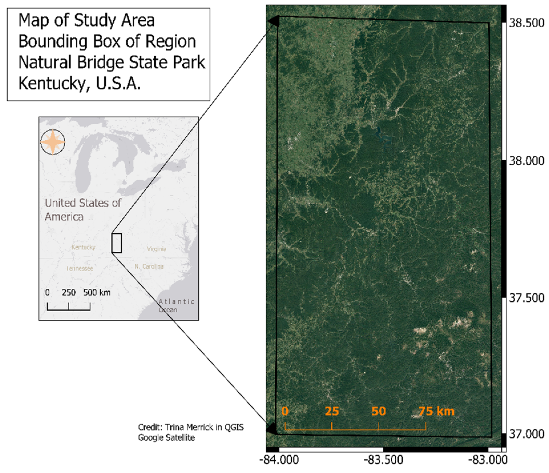
2.1. Study Site Description

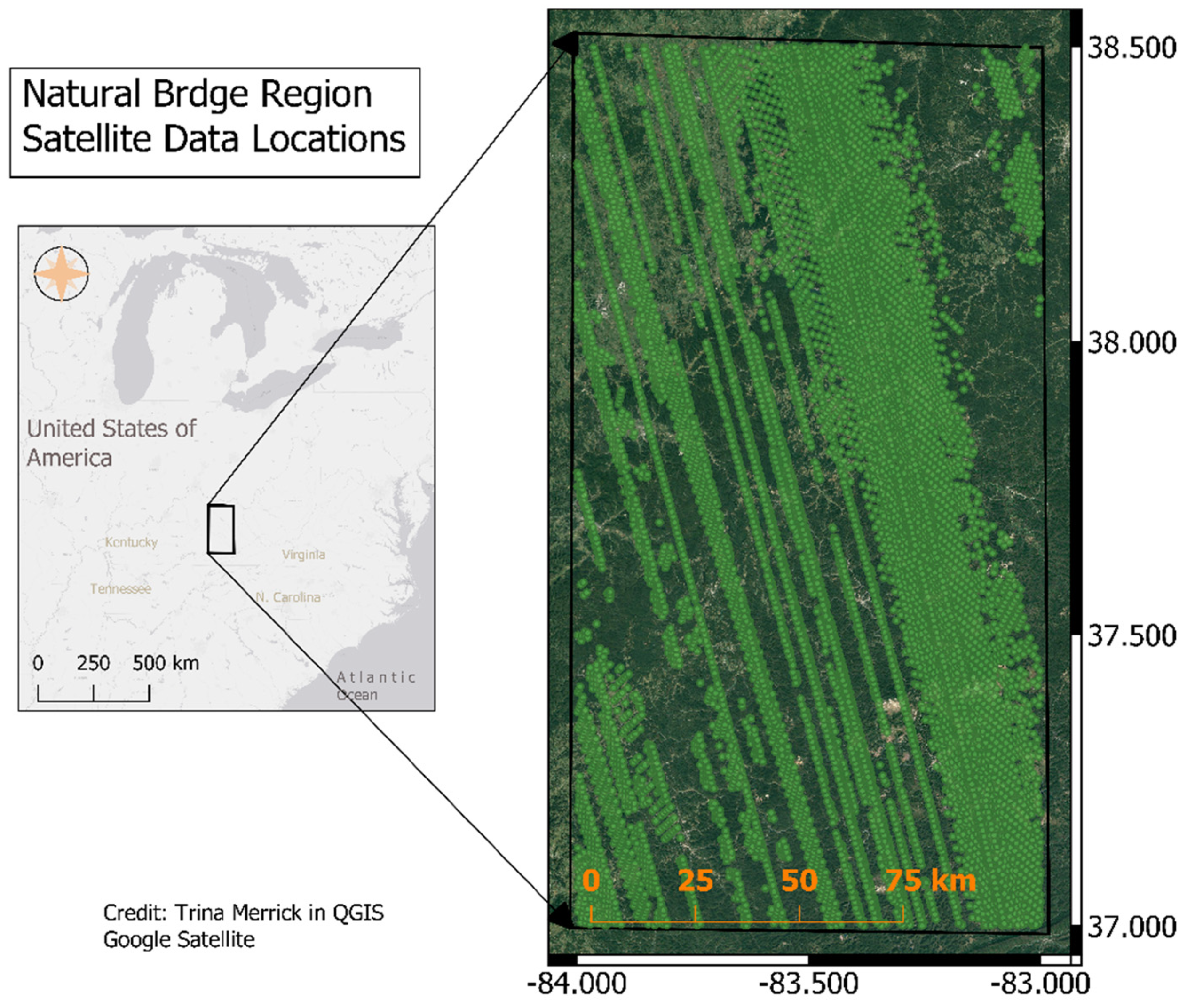
Data were extracted for the region of interest surrounding the Natural Bridge State Park near Stanton, KY, USA. (37°46′39″N 83°41′37″W, Figure 1). Mean annual air temperature is 13 °C, and mean annual precipitation is 1330 mm. The hottest month is typically July, with an average high of 29 °C and low of 19 °C, and coldest month is typically January, with an average high temperature of 7 °C and low temperature of −1.5 °C. The forest is considered a temperate deciduous forest type of the Mixed Mesophytic Region, where the climate is temperate, humid, and continental [66,67]. The location is within the Appalachian Mountains on the Cumberland Plateau on the western escarpment, making up a portion of the Red River Gorge Geologic area. The canopy is made up of a variety of oaks, pine, red maple, and other species that are leafless from late November to late March. The understory is densely dominated by species from the family Ericaceace [66,67]. The land use in the region is mainly recreational, with rock climbing, hiking, fishing, kayaking, and canoeing bringing over one million visitors, accommodating approximately 15,830 at a time (https://www.fs.usda.gov/recmain/dbnf/recreation, accessed on 22 September 2023). The Kentucky Division of Forestry asserts that eastern Kentucky forests are resilient and growing; thus, they could remain positive economic and climate mitigating factors offsetting pressures of visitors, fragmentation, severe droughts in recent years (e.g., 1988, 1999–2000, and 2007–2008, 2010, 2012, and 2016), and destructive insects (Emerald Ash Borer Beetle and Hemlock wooly adelgid; https://www.wkyufm.org/environment/2019-09-24/in-kentuckys-forests-experts-see-a-natural-climate-solution, accessed on 22 September 2023). This study is a first step in a broader strategy to incorporate ground monitoring and field data for DBF forest health in the region.

2.2. Satellite Data

A summary of all satellite data used in this study is provided in

Table 1. Summary of satellite products used in this study.

Variable	Name	Sensor/Product	Spatial Resolution	Temporal Granularity	Units
Productivity Metrics
GPP	gross primary production	MODIS MYD17A2	500 m	8 Day	g C/m2/day
NDVI	normalized difference vegetation index	MODIS MYD13Q1	250 m	16 Day	none
EVI	enhanced vegetation index	MODIS MYD13Q1	250 m	16 Day	none
SIF	solar-induced fluorescence	OCO-2	~1.2 km × 2 km	16 days	Wm2/μm/sr
GPP	gross primary production	MODIS MYD17A2	500 m	8 Day	g C/m2/day
NDVI	normalized difference vegetation index	MODIS MYD13Q1	250 m	16 Day	none
EVI	enhanced vegetation index	MODIS MYD13Q1	250 m	16 Day	none
Intermediate Variables
fPAR	fraction photosynthetically active radiation	MODIS MYD15A2H	500 m	8 Day	none
LAI	leaf area index	MODIS MYD15A2H	500 m	8 Day	m2/m2
Environmental Variables
LST	land surface temperature	MODIS MYD11A2	1 km	8 Day	K
Tcan	canopy temperature	ECMWF (OCO-2)	~1.2 km × 2 km	16 days	K
Tair	air temperature	ECMWF (OCO-2)	~1.2 km × 2 km	16 days	K
VPD	vapor pressure deficit	ECMWF (OCO-2)	~1.2 km × 2 km	16 days	kPa

. Orbiting Carbon Observatory-2 (OCO-2) SIF data were used to derive SIF metrics for the study. OCO-2 was launched in 2014, and it collects high spatial and spectral resolution measurements of solar-induced chlorophyll fluorescence (SIF) globally [68]. OCO-2 collects spectral data 24 times per second, producing eight cross-track spectra covering about 2 km × 1.3 km spatially over a swath of approximately 10 km. Although the revisit period is 16 days, through 2 July 2015, each revisit alternated between glint and nadir mode, so the repeat time for nadir was 32 days. After 2 July 2015, the instrument alternated glint and nadir every orbit. While OCO-2 SIF data have high spectral and spatial resolution, individual footprints are noisy; thus, monthly averages across the study area are used in this study [23,69,70]. The locations of the SIF footprints in the study area are shown in Figure 2. SIF data were filtered for nadir observations, and footprints were classified as temperate deciduous forests according to the International Geosphere-Biosphere Programme (IGBP) landcover classification category. Instantaneous SIF (SIF_i) was calculated for each measurement by taking the average of instantaneous SIF measured at 757 nm (SIF₇₅₇) and 771 nm (SIF₇₇₁) times a factor of 1.5 based on the OCO-2 Data Product User’s Guide and the previous literature (although the factor in previous studies ranged from 1.4 to 1.7) [20,45,69]. Daily average SIF (SIF_d) was calculated by employing the daily correction factor (DCF) [17,20,23,45,69]. The DCF is a normalization factor that approximately accounts for the length of day and variability of the solar zenith angle (SZA) using pure geometric incoming light scaling for the location in ten-minute time steps. SIF_d is calculated with the following equation:

$${SIF}_d=\frac{{SIF}_i}{cos\left(SZA\right(t_m\left)\right)}{\int }_{t=t_m-12h}^{t=t_m+12h}cos\left(SZA\left(t\right)\right)dt$$

(1)

where SZA is the solar zenith angle from the OCO-2 dataset and t_m is the time of measurement [17,20,23,45,69,70,71,72]. SIF_i values, collected at ~1330 local time, should have a higher magnitude than SIF_d because SIF_d accounts for radiation changes over the daily cycle [23,70]. Both SIF_i and SIF_d values were examined in this study because of the strong influence of changing radiation on SIF. The diurnal variability of SIF and its degree of influence at satellite scales are the focus of several studies [13,46,73,74].

The Moderate Resolution Imaging Spectroradiometer (MODIS) gross primary production (GPP), normalized difference vegetation index (NDVI), and enhanced vegetation index (EVI) products were utilized as VI measurements of production. MODIS fraction of photosynthetically active radiation (fPAR) was used as an input to calculate absorbed photosynthetically active radiation (APAR) and SIF_y (Section 2.3). MODIS NDVI and EVI MODIS are products that have been used extensively because of their high correlation with phenological changes in vegetation, their relationship to GPP, and their ability to benchmark biophysical parameters and biomass changes (e.g., [50,75,76,77,78,79]). The MODIS GPP product (MOD17) model is a semi-empirical GPP product derived using other MODIS products as parameters [77]. The MODIS GPP product is a widely used product that leverages a light use efficiency (LUE) model and generally has shown good performance estimating production [77,80]. The MODIS Land Surface Temperature Product (LST) (MYD11A2) was used as measure of canopy temperature, which is an environmental factor that may drive production [50,52,81]. To achieve the best comparisons among OCO-2 and MODIS metrics, each MODIS metric location was extracted based on the matching OCO-2 footprint location and closest time and date. Only MODIS data onboard the Aqua platform were used in analyses because the overpass time matches OCO-2 (1330 local). For the purposes of this study, SIF_i, SIF_d, SIF_y, GPP, NDVI, and EVI are considered productivity metrics, and fPAR and LAI are considered intermediate variables because LAI and fPAR products from MODIS are used to model GPP from MODIS data.

To examine the relationships among SIF, GPP, and environmental factors potentially controlling photosynthetic activity in this study, skin temperature (T_can), 2 m temperature (T_air), and vapor pressure deficit (VPD) from the European Center for Medium-Range Weather Forecasts (ECMWF) available within the OCO-2 SIF dataset were used. Land surface temperature (LST) from MODIS was also collected for the study period as a second approximation of canopy temperature.

Proxies of production, i.e., satellite measurements of VIs and satellite-based SIF, were compared to one another in terms of phenology and relationships that may help inform the interpretation of SIF measurements [82,83,84,85,86,87].

2.3. Calculating SIF_y

SIF signals incorporate both the physiological (photosynthetic) response of vegetation and the physical (absorbed and scattered light). SIF normalized by the absorbed photosynthetically active radiation (APAR) has been used to better approximate the physiological photosynthetic response of vegetation more independently of the absorbed and scattered light [40,44,58]. OCO-2 SIF_d and MODIS fPAR data were used to calculate a satellite-based approximation of relative SIF yield (SIF_y). An estimated SIF_y at the satellite level was calculated according to the following equation:

$${SIF}_y=\frac{{SIF}_d}{cos\left(SZA\right)fPAR}$$

(2)

where SZA is the solar zenith angle for the associated OCO-2 SIF measurement, and fPAR is the MODIS fPAR measurement with high-quality flag most closely matching the OCO-2 SIF measurement date.

2.4. Data Analysis

Area-based monthly averages were calculated for SIF metrics and VIs: SIF_i, SIF_d, SIF_y, GPP, NDVI, and EVI and environmental factors: LST, VPD, T_can, and T_air for the time period September 2014 to August 2018 (48 months). Time series of monthly values and anomalies for the full 48 months of data were calculated to examine interannual variability. Within the region, the occurrences of moderate to severe drought in 2016 were anticipated to be detectable in the signals. Average annual cycles, i.e., the mean of all measurements made in each of the twelve months of the year for all years of data [3,5,8], were used to examine seasonal differences in SIF metrics, VIs, and environmental factors. Altogether, five different types of analyses were conducted to compare SIF metrics and VIs and examine environmental drivers: long-term time series, average annual cycles, correlations, multiple regression, relative importance of variables, and seasonality analysis. Specifically, the strength and direction of relationships among SIF_i, SIF_d, SIF_y, GPP, NDVI, EVI, LST, VPD, T_can, and T_air were investigated using Pearson correlation for the time period September 2014 to August 2018 (48 months) and bivariate plots with trend lines to examine the relationships of individual SIF metrics and VIs to environmental variables. Relative importance of the environmental variables on productivity was measured using multiple regression techniques, specifically the LMG method, also known as a dominance-type method, or Shapely value regression [88,89] and bootstrapping (1000 iterations), used to calculate confidence intervals as a guide to the significance of the differences in relative importance. In addition, partial least squares regression was applied to calculate the relative importance, with no significant difference in the result compared to LMG.

The TIMESAT algorithms were used to gap-fill and smooth the signals and determine seasonality parameters with SIF_i, SIF_d, GPP, NDVI, and EVI as inputs [51,90,91]. TIMESAT was designed to analyze time series data from satellite sensors and generate seasonality parameters. Seasonality parameters calculated from the analyses include start of season (SOS), end of season (EOS), peak of season, season length (LOS), base value, maximum value, amplitude value, rates of increase and decrease, large (total) integrated value, and small (pulse) integrated value. Double logistic function fitting was applied within the TIMESAT algorithms to time series of SIF_i, SIF_d, SIF_y, GPP, NDVI, and EVI. The average of the seasonality metrics for the seasons detected over the four-year period in each time series was calculated to represent the seasonality parameters of each quantity. The algorithm determines the base as the average of the left and right minimum values and the amplitude as the difference between the base value and the maximum. The times for the beginning and end of season are determined using 0.5 of the amplitude from the left and right, respectively, following methods for determining seasonality parameters in the literature [49,51,63,65]. The resulting normalized base-integrated production (the base determined from TIMESAT results) and the pulse-integrated production (the amplitude determined from TIMESAT results) for each quantity were compared. The length of season (LOS) in days and the beginning and end of season (BOS and EOS, respectively) in the day of year (DOY) were extracted, and the differences between BOS, EOS, LOS, base, and pulse-integrated production (as values and percentages) were examined.

Code to read, process, and analyze OCO-2, MODIS, and ancillary data was developed using Interactive Data Language (IDL, Harris Geospatial, Boulder, CO, USA). TIMESAT algorithms were used, as previously mentioned, to calculate metrics of seasonality [51,90,91]. Functions within the R package MODISTools version 1.1.1 were used to assist in accessing matching study area OCO-2 footprint locations to MODIS data from Aqua, and a combination with R and IDL functions were used for quality assurance, applying correction and multiplier values, and generating time series data for the study period [92,93]. All statistical analyses and figures from statistical and seasonality analysis were completed in IDL and R, RStudio version 1.0.153, and the following packages: dplyr, tidyverse, ggplot2, corrplot [94,95,96,97,98].

3. Results

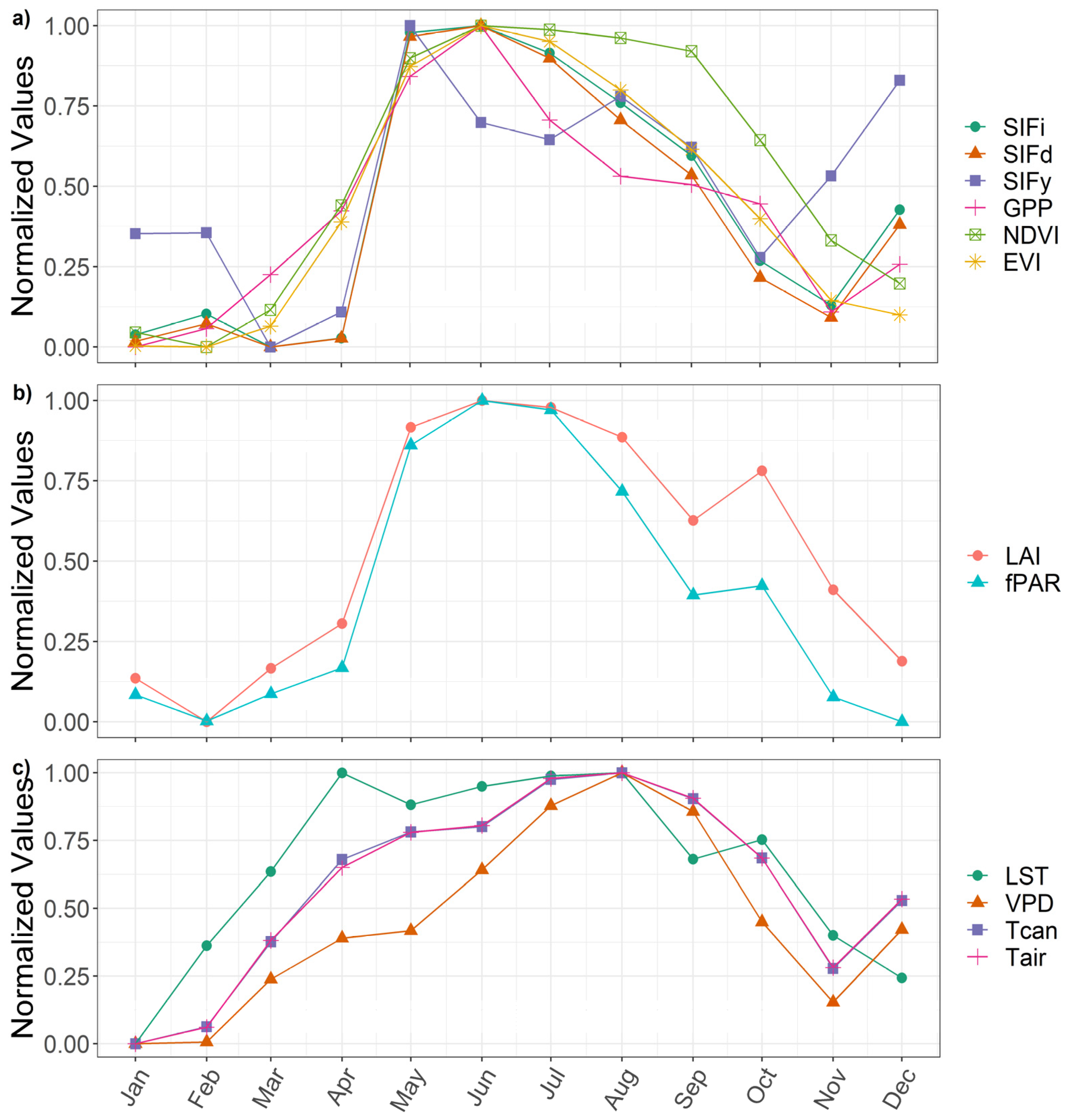
3.1. Examine Time Series and Annual Cycles

All productivity metrics (SIF_i, SIF_d, SIF_y, GPP, NDVI, and EVI) and intermediate variables (fPAR and LAI) display seasonal cycles each year, with the highest values occurring in summer and the lowest values occurring in winter months, except for SIF_y. (Figure 3). SIF_i, SIF_d, and GPP peak values occurred most often in May (2015, 2016, and 2017), except in 2018, when GPP still peaked in May but SIF_i and SIF_d peaked in June (Figure 3a–c). While the peak month for EVI tended to be in June rather than May (Figure 3), the trend of sharp peaks was similar to SIF_i, SIF_d, and GPP (Figure 3f). NDVI did not exhibit sharp peaks; rather, it remained at similar values for the summer months before dropping quickly to low levels during the winter months (Figure 3d). NDVI peaked in different months for each year of the analysis: July 2015, May 2016, August 2017, and June 2018 (Figure 3d). GPP, NDVI, and EVI values declined to low values mainly in January or February, after which they increased into the summer (Figure 3b,d,f). SIF_i and SIF_d, however, reached low values in the fall and then experienced a relatively small peak once each winter (Figure 3a,c). SIF_y displays little indication of seasonality matching the other measures of productivity and large standard deviations in portions of the time series compared to SIF_y values, i.e., SIF signal is composed largely of fPAR and the remaining information is noisy (Figure 3e). LAI and fPAR, the intermediate variables, display patterns of high values in the summer months and low values in the winter months, similar to the other MODIS products (Figure 3g,h). In January 2017, the monthly mean LAI and fPAR were higher than in December 2016 and February 2017, but with a particularly high standard deviation in these metrics.

A time series of LST, T_can, T_air, and VPD highlights the seasonal variation of these environmental factors in the temperate deciduous forest in all cases (Figure 4). The T_can and T_air patterns were the same. The peak months of VPD matched the peak months of T_can and T_air, but the patterns during the winter and spring were more distinct for VPD than for T_can and T_air. Generally, there was a slower increase in VPD relative to the peak month of VPD than for LST, T_can, and T_air, which sharply rose after winter and remained closer to their peak for a few more months, and then declined more sharply in the fall. The monthly LST from MODIS reflected a similar pattern to T_can and T_air, and, although the overall range of the temperature was similar, the values of LST were higher than those for T_can and T_air. All the time series, including productivity metrics, intermediate variables, and environmental factors, were examined for anomalies and extreme values, but none were found for the study period.

The annual average cycles (normalized) represented typical seasonal behavior and show that the peak values of productivity occur in June for all measures except SIF_y, which peaks in May (Figure 5a). SIF_i, SIF_d, and SIF_y reach their minimum values in March; NDVI and EVI reach their minimum values in February, but GPP reaches its minimum value in January, a likely result of the minimum values of LAI and fPAR occurring in February and December, respectively (Figure 5a,b). SIF_i and SIF_d have the most similar trend. EVI trends similarly to SIF_i and SIF_d from the peak months to October and November. GPP trends with EVI and NDVI in the spring, although it increases more rapidly in March, peaks with everything except SIF_y in June, and declines more rapidly in August. GPP, SIF_i, and SIF_d all experience an increase from November to December before reaching their minimum values in January, while SIF_y trends up from October to December and declines to a minimum in March. From May to September, NDVI remains at similar values, while the other measures of productivity display more variability throughout the growing season. LAI and fPAR reach relatively high and similar values in May through July, peaking in June (Figure 5b).

While the trends are similar for the year, LAI and fPAR reach their minimum values two months apart (February and December, respectively), deviating most from one another from August to December (Figure 5b). LST, VPD, T_can, and T_air are all at their minimum values in January and maximum values in August (Figure 5c), with LST also reaching its maximum value in April. LST increases more rapidly than the other environmental variables through April, and then it dips slightly between its months with the maximum values (April and August, Figure 5c). T_can and T_air trend together, almost identically, with a small separation in April. VPD remains at the minimum for January and February and increases less rapidly than other environmental variables before reaching the maximum in August. After August, VPD, T_can, and T_air trend down more similarly than LST, decreasing through November and then increasing in December before reaching the minimum in January. LST drops from August to September, rises slightly in October, and then decreases to its minimum value in January.

3.2. Correlations

The productivity metrics SIF_i, SIF_d, GPP, NDVI, and EVI are all strongly positively correlated (Pearson correlations, r values between 0.84 and 1.00, p < 0.001,

Table 2. Correlations among SIF_i, SIF_d, SIF_y, GPP, NDVI, EVI, LAI, and fPAR (Pearson, r-values. *** indicates p-value < 0.001; ** indicates p-value < 0.01).

Value	SIFi	SIFd	SIFy	GPP	NDVI	EVI
SIFd	1.00 ***
SIFy	0.67 ***	0.65 ***
GPP	0.85 ***	0.86 ***	0.43 **
NDVI	0.84 ***	0.84 ***	0.46 **	0.84 ***
EVI	0.89 ***	0.89 ***	0.48 **	0.88 ***	0.96 ***
LAI	0.76 ***	0.76 ***	0.42 **	0.80 ***	0.87 ***	0.85 ***
fPAR	0.82 ***	0.82 ***	0.42 **	0.84 ***	0.82 ***	0.88 ***

). Correlations between SIF_i and GPP (r-value = 0.86, p < 0.001, Table 2) as well as SIF_d, and GPP (r-value = 0.86, p < 0.001, Table 2), NDVI and GPP (r-value = 0.84, p < 0.001, Table 2), and the EVI~GPP correlation (r-value = 0.88, p < 0.001, Table 2) were all very similar. Besides the correlation between them, SIF_i and SIF_d had the strongest correlation with EVI (r-values = 0.89, p-value < 0.001, Table 2). SIF_y correlations with the other productivity metrics were positive and significant, but they were the lowest correlations of the SIF metrics, and the relationship between SIF_y and other metrics was very low (r-values between 0.43 and 0.67, p < 0.01, Table 2). Correlations between LAI and both SIF_i and SIF_d were strongly positive (r-value = 0.76, p-value < 0.001, Table 2), and fPAR was slightly more strongly correlated to SIF_i and SIF_d (r-value = 0.82, p-value < 0.001, Table 2). LAI and fPAR were only moderately positively correlated with SIF_y (r-value = 0.42, p-value < 0.01, Table 2). LAI was most strongly correlated with NDVI (r-value = 0.87, p-value < 0.001, Table 2), and fPAR was most strongly correlated with EVI (r-values = 0.88, p-value < 0.001, Table 2).

Relationships among environmental variables were positive, with p-values < 0.001 (

Table 3. Correlations among environmental variables examined in the study: VPD, T_can, and T_air (Pearson, r-values. *** indicates p-value < 0.001).

Value	VPD	Tcan	Tair
Tcan	0.88 ***
Tair	0.88 ***	1.00 ***
LST	0.64 ***	0.76 ***	0.76 ***

). T_can and T_air have the strongest relationship (r-value = 1.00). T_can and T_air had a strong positive relationship with VPD, with an r-value of 0.88 (Table 3). Relationships between environmental variables from the two different datasets (ECWMF data and MODIS) had weaker relationships. LST~VPD was 0.64, and LST~T_can and T_air were 0.76 (Table 3).

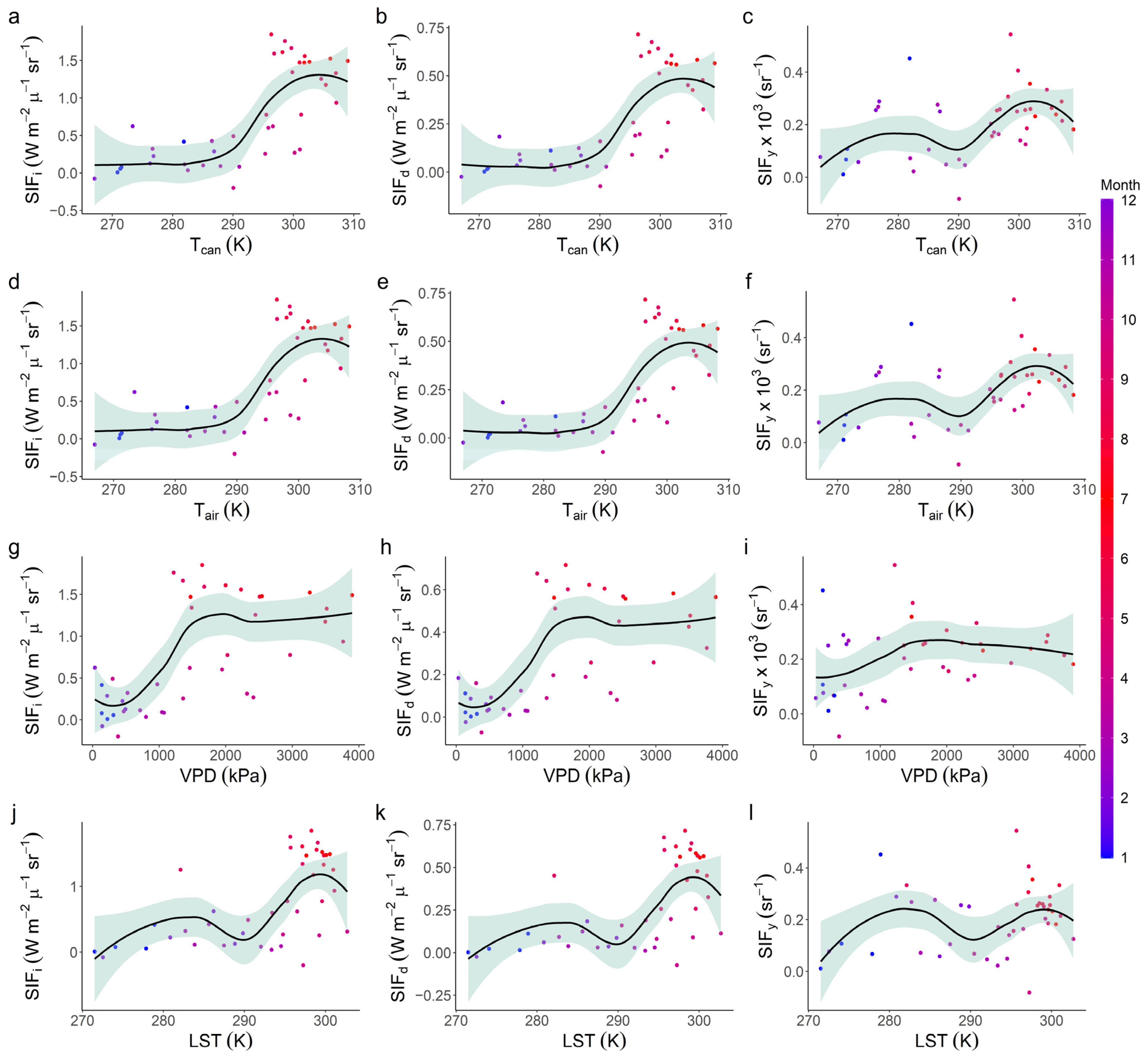
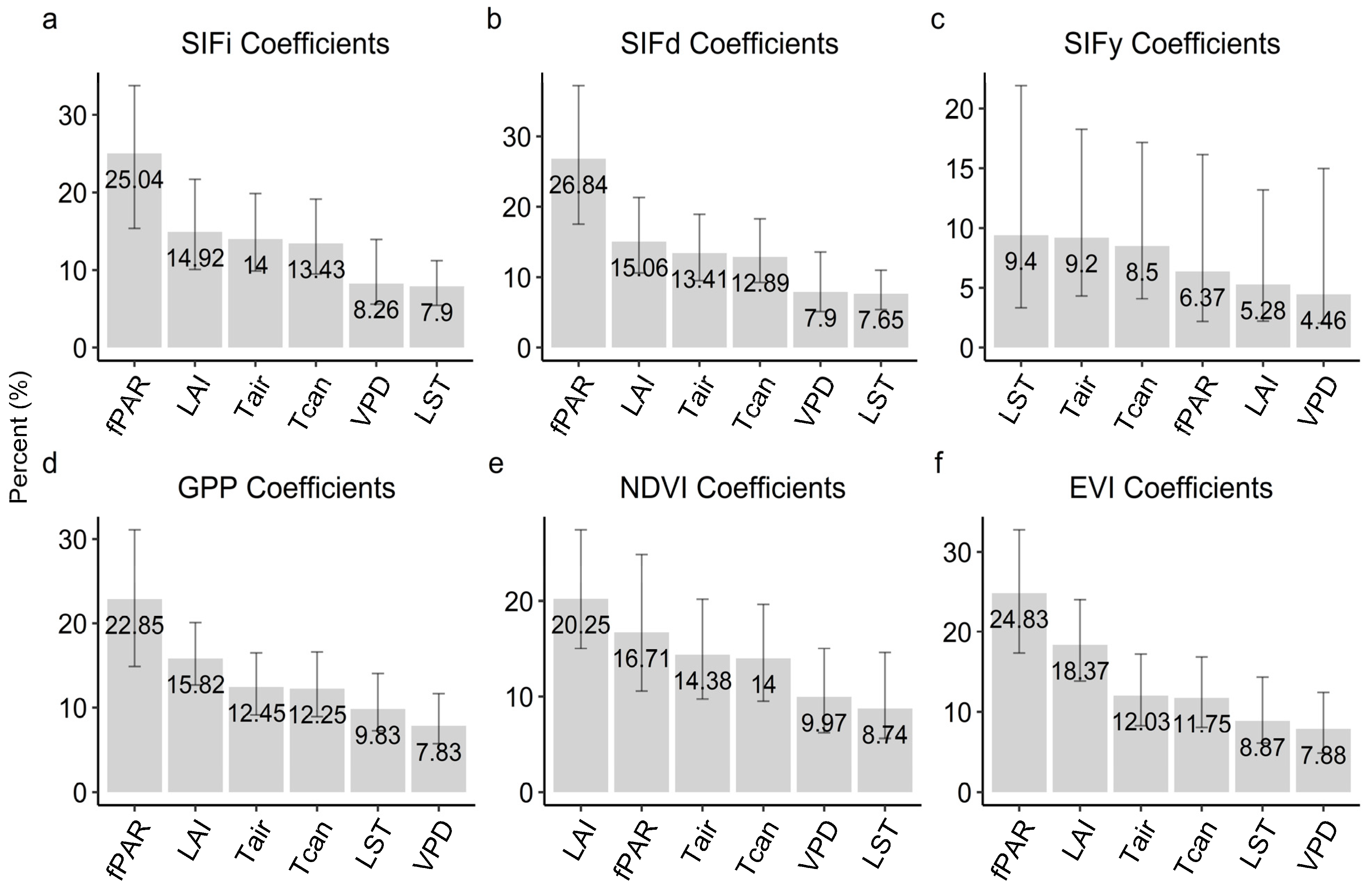
3.3. Relationships with Environmental Factors

Figure 6 and Figure 7 illustrate relationships between environmental factors and productivity metrics, with the color of the data points representing months (winter months in purple and summer months red). Temperatures T_can, T_air, and LST display similar trends with SIF_i and SIF_d, despite a larger range of T_can and T_air values attributed to higher values versus LST (Figure 6a,b,d,e,j,k). SIF_i and SIF_d vs. T_can, T_air, and LST trends are flat in the winter months, and then they climb in spring and reach the maximum values, followed by a distinct decrease at the hottest temperatures (Figure 6a,b,d,e,j,k). SIF_i and SIF_d vs. VPD trends show clustering in the winter months and summer peak earlier than that for temperatures, followed by slowly decreasing trends at the highest VPD (Figure 6g,h). SIF_y–environmental variable trends share some general features with those of SIF_i and SIF_d–environmental variable trends; however, SIF_y outliers affect the trends (Figure 6c,f,i,l). In all cases, the relationships are not linear in nature, but there is a great deal of scatter among the SIF metrics and environmental variables (Figure 6).

Trends among VIs and environmental variables (Figure 7) indicate that GPP reaches a maximum before the hottest months and then decreases at high T_can, T_air, and LST (Figure 7a,d,j). NDVI and EVI tend to saturate at high T_can and T_air, although NDVI values cluster more tightly at the highest T_can and T_air than EVI values (Figure 7a–f,j–l). Driven by an outlier, NDVI and EVI~LST trends appear to reach their maximum values before the hottest months and then decrease at the highest LST value, without which these trends would also cluster and saturate similar to NDVI, EVI~T_can, and T_air (Figure 7a,d,j).

The relative importance of environmental variables in predicting productivity metrics was conducted in two ways. First, the analysis was conducted only with the environmental variables T_can, T_air, VPD, and LST, and then again with the four environmental variables plus the intermediate variables fPAR and LAI. The results presented here include the group of environmental variables plus the intermediate variables because the variance of productivity explained with only environmental variables was 34.9–70.89%, while adding the intermediate variables improved the variance to 43.2–84.1%. The variance explained by the environmental variables plus intermediate variables in this study is as follows: SIF_i 83.56%, SIF_d 83.75%, SIF_y 43.22%, GPP 81.02%, NDVI 84.06%, and EVI 83.73%. All metrics of productivity were similarly well explained by these predictors, except SIF_y, which was not well explained by these predictors. SIF_y is included in Figure 8 for informational purposes but is excluded from the detailed results.

fPAR was the most important for predicting productivity metrics (22.9–26.8%; Figure 8a,b,d,f), except for NDVI, where LAI was most important (20.25%; Figure 8e). However, LAI and fPAR do not differ significantly in terms of their influence on NDVI, according to the confidence intervals. For SIF_i and SIF_d, fPAR was significantly more influential than LAI, T_can, and T_air, which all have the same relative importance. For GPP and EVI, fPAR was significantly more influential than the other variables, and LAI was somewhat more influential but only marginally significant. Figure 8 shows that the intermediate variables, fPAR and LAI, are the most influential on the metrics of productivity compared to the environmental variables. T_air was the strongest predictor among all the environmental variables (12–14.4%; Figure 8). However, T_air was only slightly more influential than T_can (11.8–14.0%; Figure 8) in all cases, and the confidence intervals show that these predictor variables have no significant difference in influence. Furthermore, for all productivity metrics, LST and VPD were the lowest in relative importance and not significantly different (7.7–10.0%; Figure 8). Even considering the confidence intervals, it is shown that fPAR is the most influential variable on SIF, a concept that is documented in other studies. In this study, a calculation of SIF_y was tested as a proxy of productivity independent of fPAR, which Figure 8c illustrates.

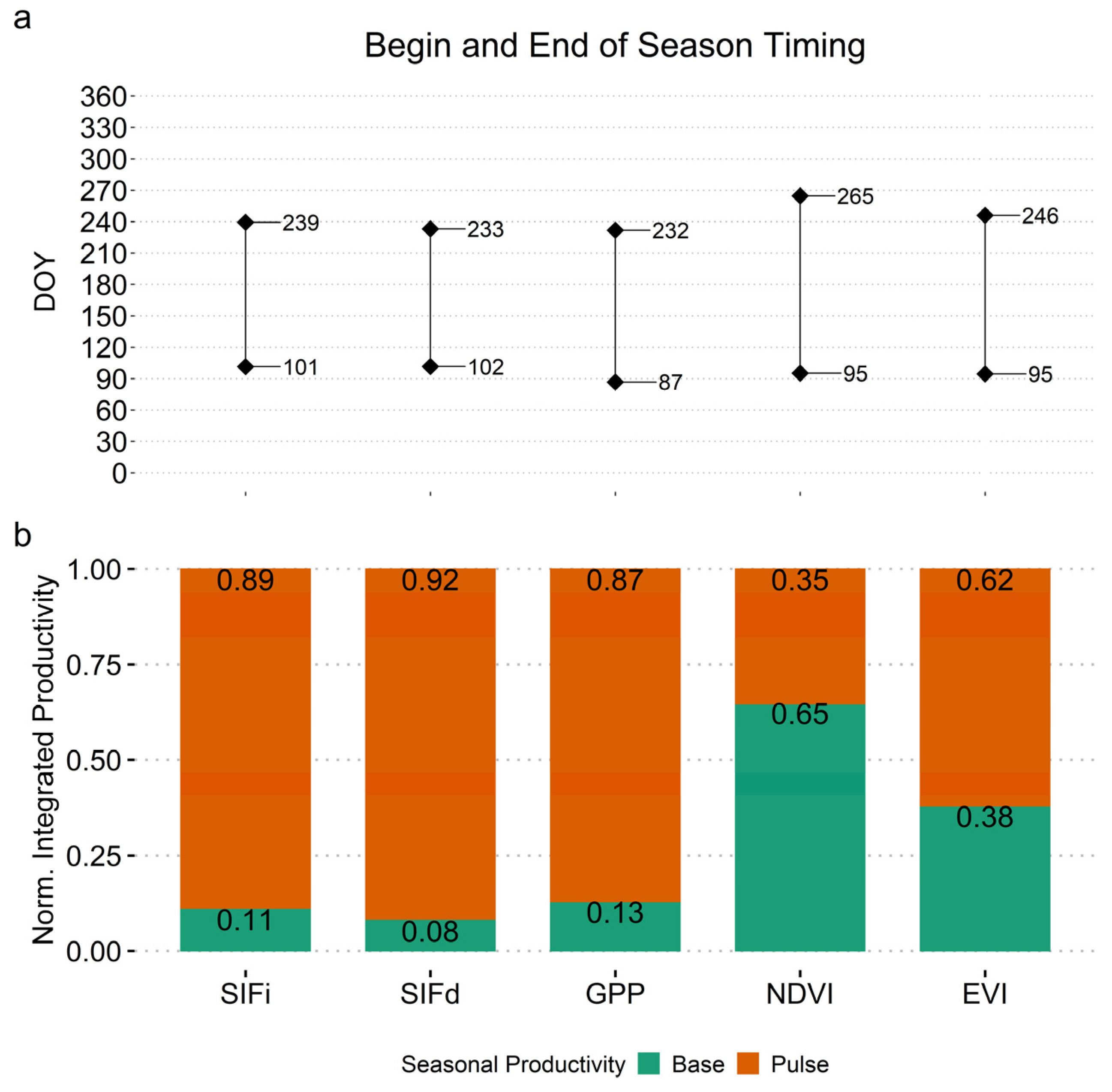
3.4. Seasonality Analysis

The estimates of the length of the season (LOS), indicated by different productivity metrics, differed by as much as 48 days (Figure 9a). SIF_d indicated the shortest growing season (132 days), followed by SIF_i (138 days), GPP (145 days), EVI (152 days), and NDVI (170 days). The SOS and EOS timings estimated with SIF_i, SIF_d, GPP, and EVI were within two weeks of one another, indicating shifts of a few days in the season start and end times among the metrics (Figure 9a). GPP had the earliest start and end dates. In contrast, NDVI had a similar SOS, but the EOS was two weeks or more after the SIF_i, SIF_d, GPP, and EVI EOS. NDVI indicated the longest growing season due to the later EOS (18 to 38 days longer).

The proportion of integrated production attributed to the base and pulse-integrated production for SIF_i, SIF_d, and GPP was comparable (base = 0.11, 0.08, and 0.13; pulse = 0.89, 0.92, and 0.87, respectively; Figure 9b). Normalized estimates of base and pulse-integrated production estimated by SIF_i, SIF_d, and GPP indicated that the base production for the study area was between 0.08 and 0.13 of the total production (or about 8–13%) and the seasonal pulse-integrated production was responsible for 0.87 to 0.92 (87% to 92%) of the deciduous forest production (Figure 9b). In contrast, NDVI indicated that the base production was 0.65 and the pulse was 0.35 (65% and 35%, respectively). EVI had an intermediate estimate of the base (0.38) and pulse (0.62) integrated production. SIF_y seasonality metrics are excluded from the seasonality results because repeated tests of seasonality calculations for SIF_y did not yield consistent or reliable results, which was likely due to the lack of seasonal cycles present for SIF_y.

4. Discussion

In this study, a seasonality analysis revealed differences in how the phenology of temperate forest canopy production can be represented by different remote sensing proxies. Studies have shown that EVI, GPP, and especially SIF are more indicative of physiological responses of vegetation to the environment than NDVI [99,100], but relatively few studies have examined the seasonality of EVI, GPP, or SIF compared to NDVI (e.g., [5,51,63,101,102]). Here, seasonality measurements were based on SIF_i, and SIF_d allocated production to the base and growing season pulse in similar proportions to GPP. SIF_i and SIF_d signals are known to incorporate both physiological (photosynthetic rate) and physical information (light absorption and SIF scattering) about the vegetation canopy (e.g., [13,32,33,42,103,104,105]. GPP from MODIS is fundamentally a different satellite remote sensing measurement whose model incorporates LAI, fPAR, VIs, and information on vegetation type [51,106,107,108]. Despite the fundamental differences in measurements of SIF from OCO-2 and GPP from MODIS, a strong agreement in production and timing between them is evident. This agreement may stem from a correlation between the radiation information contained within the SIF signal and the inclusion of fPAR in the MODIS GPP algorithm. Additionally, GPP from MODIS could be used in tandem with OCO-2 SIF for spatial and temporal gap filling, for further seasonality and phenology studies, as tools for monitoring vegetation changes in a changing climate and developing new productivity datasets using OCO-2 SIF and MODIS GPP products similar to those presented by Zhang et al. [109].

In this study, different satellite-based productivity metrics, intermediate variables, and environmental factors were investigated to determine how they captured the productivity and phenology of a DBF on a regional scale using a range of analyses, from more reliant on visual inspection to more quantitative. The inspection of time series and intra-annual cycles of SIF metrics (SIF_i, SIF_d, and SIF_y), VIs (GPP, NDVI, and EVI), intermediate variables (fPAR and LAI), and environmental variables (LST, T_can, T_air, and VPD) displayed expected trends of changes corresponding to the growing and non-growing seasons, except SIF_y (Figure 3 and Figure 4). NDVI maintained similar values throughout the growing seasons, while other productivity metrics showed more variability, especially during spring and fall (Figure 3a). This is consistent with previous studies, where NDVI has been shown to saturate in the growing season (e.g., [69]). Visual inspection of normalized annual cycles also revealed NDVI differences from SIF metrics and EVI, especially higher values in the late summer and early fall months. Normalized annual cycles were also the first step to examine the potential influence of environmental variables and the timing of seasonal changes. For instance, the environmental variables peaked in August, while the productivity metrics peaked in earlier months, which could be due to a high temperature threshold after which productivity tends to decrease (e.g., [50], Figure 4a–c).

An analysis of the time series and normalized annual cycles revealed no anomalies, despite a known drought occurring in 2016. This result indicates that the resolution, either spatial, temporal, or both, was insufficient for detecting drought-induced changes for this event for a DBF using any of the metrics. As suggested by previous studies, SIF metrics have increased sensitivity for monitoring stress over VIs, but they currently vary in the degree to which events are detectable due to spatial or temporal scales and regions e.g., [24,35,100,101]. Using the methods in this study, OCO-2 SIF did not benchmark the event at this juncture. In our upcoming work, however, revised methods or more recent satellite platforms and products, which are increasing exponentially, promise to benchmark such events in DBF.

Correlations provided basic quantification of the relationships among the SIF and VIs, which were generally strong, positive relationships, except for SIF_y (Table 2). These results are in alignment with earlier studies that have found strong relationships between SIF and satellite GPP, NDVI, and EVI using time series, annual cycles, and correlations (e.g., SIF correlated with EVI (r = 0.69) and NDVI (r = 0.6 to 0.69) and SIF correlated with GPP (r = 0.89 to 0.99)) [17,69,99,100]. However, the strong correlations do not have the capacity to quantify differences in productivity metrics in terms of timing, which were seen in the normalized annual cycles (Figure 4a–c). Furthermore, correlations that have been used in the context of relating VIs to both satellite-based GPP and ground station GPP from flux towers have not often incorporated finer-scale seasonal timing and phenology. As mentioned in the recent literature (e.g., [3,5,33,35,59]), if the examination of relationships stopped with correlations, it would appear as if SIF_i, SIF_d, GPP, NDVI, and EVI would serve as near equal proxies of GPP, but when paired with time series and other information related to timing, such as subsequent analyses in this study, the relationships change. For instance, the bivariate scatterplots reveal nonlinear relationships that change throughout the year (Figure 6 and Figure 7).

Bivariate scatterplots (Figure 6 and Figure 7) show that SIF metrics, GPP, and EVI peak at temperatures just below maximum, and then they experience lower values of productivity at maximum temperatures. NDVI, however, saturates in the warm months. These results are consistent with studies that found that SIF is more sensitive to changes in function than NDVI [3,8,15,17]. All productivity metrics, including NDVI, show more similar relationships to VPD. In a few studies that have examined satellite-based SIF or Vis relationships with VPD, SIF has been more sensitive to VPD and associated water and heat stress than Vis (e.g., [110,111,112]). The results, however, show that the scale of the satellite-based productivity metrics and the environmental data available (modeled and included in the remotely sensed data, except LST) were not able to capture the regional water stress that may have existed during 2017 drought conditions (Figure 6g–i and Figure 7g–i). It was anticipated that by examining regional-scale environmental factors and using footprint-level comparisons of satellite-based productivity, SIF would capture this event and outperform VIs to a greater degree. But the results demonstrated that there was not sufficient information to capture subtle behavior within the same biome type or at regional scales, which is consistent with studies examining other biome types at different spatial and temporal scales ([3,6,30,39,40]; Figure 6 and Figure 7). Instead, as suggested in [69], these subtleties and complexities require quantification for specific vegetation types and environmental conditions within the context of phenology and environmental variables that drive changes in these metrics [3,8,18,60,62,65].

A time series of environmental factors, T_can, T_air, VPD, and LST, as well as intermediate variables (fPAR and LAI), were investigated due to their potential roles as drivers of change in productivity. Environmental and intermediate variables’ time series plots and intra-annual cycles generally showed similar trends to those of SIF metrics and VIs, but some with leading or lagging patterns of minimum and maximum timing (Figure 3, Figure 4 and Figure 5). To more quantitatively understand the relationships beyond correlations and trends, an analysis of the relative importance of variables indicated that SIF metrics and VIs were most influenced by intermediate variables, fPAR and LAI, followed by temperature (Table 2 and Table 3, Figure 6, Figure 7 and Figure 8). Previous studies using finer resolution data suggest that forest GPP is more tightly coupled to canopy temperatures than air temperatures, but at the coarse resolution of this study, T_can and T_air exert a similar influence on SIF metrics and VIs (Figure 8). In contrast to the other environmental factors, LST from MODIS did not generally have as great an influence on productivity metrics, but the trends were similar for the three types of temperature measurements (Figure 6, Figure 7 and Figure 8). MODIS LST has been widely used and validated using ground data, models, and cross-comparison to other satellites [113,114,115,116]. LST was shown here to perform similarly to the other temperature metrics for explaining VIs in DBNF for the study period but not for SIF metrics.

Seasonality analysis quantifies similarities and differences in productivity measured with these remote sensing metrics. SIF metrics had the shortest season of productivity, about one week shorter than GPP, two weeks shorter than EVI, and over two weeks shorter than NDVI, which corresponds to the relative base and pulse-integrated productivity (Figure 9). In the case of SIF metrics and GPP, the EOS DOY was almost identical; therefore, the difference in relative integrated productivity was attributed to an earlier GPP SOS. For SIF and EVI, the relative integrated productivity difference was due to both an earlier EVI SOS (just under one week) and a later EVI EOS (just under one week). Thus, differences in production measured with SIF metrics, GPP, EVI, and NDVI are not explained by simple differences in LOS for each quantity; rather, these satellite-based proxies are complex representations of the physiological and physical responses of vegetation. The SOS and EOS shifts, together with the integrated productivity results, suggest that SIF metrics and GPP versus EVI versus NDVI capture varying degrees of phenological and structural changes at different timings (Figure 9).

The results show that SIF_i, SIF_d, GPP, and, to some lesser extent, EVI, respond to the same or coincident temperate forest vegetation production dynamics, such as canopy structural changes, light capture and scattering, and photosynthetic responses to the environment. Canopy level field measurements of the Natural Bridge area within DBNF during a period of NDVI senescence also indicate that EVI and NDVI capture different trends and variability and agree well with satellite data, but they were too few and spatially limited to directly validate the satellite scale reflectance measurements. Furthermore, as longer records of SIF, such as from OCO-2, OCO-3, and the TROPOspheric Monitoring Instrument (TROPOMI) aboard the Copernicus Sentinel-5P mission, become available, GPP, SIF, EVI, and other satellite-derived datasets, as well as more refined estimates of SIF_y, can be used in tandem to improve our understanding of production estimates, as model inputs, and to spatially and temporally gap-fill data, as well as create new datasets to track vegetation dynamics with satellite remote sensing observations.

SIF metrics, GPP, and EVI to a more moderate degree, indicate a more complex representation of drivers and responses than NDVI. The differences in relative integrated productivity derived from SIF versus NDVI can be attributed to NDVI SOS, which was just under a week earlier than SIF SOS, but NDVI EOS was approximately one month later than SIF EOS (26 and 32 days; Figure 9). NDVI showed the least agreement with all the other indicators of relative base or pulse-integrated production and LOS, indicating changes into senescence much later in the year. When relying on correlations, for instance, clustering of NDVI values, for instance, by season could indicate strong relationships with GPP and other productivity metrics. It is because of this strong correlation that NDVI is heavily relied upon in studies of vegetation productivity and seasonality, e.g., [47,62]. However, seasonality analyses add to the growing body of research showing that SIF captures more information regarding the function of vegetation, while NDVI indicates changes in structure [18,33,34,100,104]. Furthermore, EVI and GPP from MODIS demonstrated more similar capturing seasonality to SIF than NDVI (e.g., [17,18,75,76,77]). Also, NDVI correlation behavior might disappear in vegetation with less variation in seasonal temperature (tropics) or vegetation with fewer structural seasonal changes (evergreen), which supports findings in previous studies, e.g., [43,62,89,99,106]. Taken together with the evidence from other studies (e.g., [17,18,27]), NDVI likely responds to the most pronounced changes in the structure of the forest canopy combined with increasing soil and background. While NDVI is an often-used metric for seasonality analysis, it was found to provide the least information beyond the most pronounced structure changes [17,18,22,23]. In contrast, EVI captured deciduous vegetation changes missed by NDVI through the exploitation of the NIR and additional blue spectral region. The proportion of production for the base and growing seasons indicated by EVI was more similar to GPP than NDVI, although it was not as similar as SIF to GPP. EVI also indicated a relatively larger pulse-integrated production than NDVI, even though the LOS for NDVI was approximately 18 days longer. EVI achieved this likely because of reduced atmospheric and soil background effects and less saturation than NDVI [7,48,59,89]. These results indicate that seasonality analysis using EVI has potential applications in tracking vegetation phenology beyond that of NDVI and may be more comparable to SIF and GPP. Taken together with the widespread availability and long record of satellite EVI, EVI remains a valuable and relevant source of phenological information.

The agreement between SIF_i, SIF_d, and GPP may stem from the greater sensitivity of these remote sensing proxies to changing environmental factors than NDVI or EVI. The GPP product from MODIS incorporates information regarding environmental conditions via a model, and SIF has proven to be sensitive to light and environmental conditions (e.g., [3,8,10,12,14]). For instance, NDVI clusters for cool versus warm months to a greater degree than GPP or SIF metrics and saturates in the growing season (Figure 6 and Figure 7). As mentioned previously, NDVI correlations that exist with SIF indices are likely driven by seasonal clustering rather than tracking incremental changes. SIF metrics and GPP are more evenly distributed across the months in response to changes in T_can and T_air, as well as VPD, which illustrates that SIF_i, SIF_d, SIF_y, GPP, and even EVI capture more subtle responses of the forest to environmental factors than NDVI. This can be especially applicable in phenological studies or monitoring ecosystem responses related to changing climates [4,7,117,118].

A method to estimate SIF_y using OCO-2 and MODIS fPAR was tested. A technique to reliably calculate SIF_y using satellite data would open the possibility of greater photosynthetic information available at the greatest spatial scales. However, the SIF_y time series resulted in unreliable seasonality calculations; thus, no phenological insights or improved interpretation of SIF patterns were found. The SIF_y result indicates that the SIF signal is composed largely of fPAR and the remaining information is noisy (Figure 3e). The calculation did, however, remove the influence of fPAR as indicated by the relative importance of variable analysis (Figure 8), but it is suspected the remaining data are not helpful for the interpretation of SIF and its relationship to carbon uptake. This estimate of SIF_y may provide a starting point to explore the physiological response of the canopy using other satellite-based data to enable studies where field- or tower-based data are unavailable. For a future study, it is possible that including a larger area and a longer time series using this or an updated version of estimating SIF_y could improve SIF_y seasonality metrics and, thus, the interpretation of the SIF connections to GPP (e.g., [42,43,44,99]). In addition, including field measurements of fPAR, PAR, and irradiance generally would be of great interest but was not available in this limited study. In studies where data are available to compare GPP or light use efficiency (LUE) from fields or towers, SIF yield is revealing important biome and species-specific functions (e.g., [3,12,17,20]). A satellite-based SIF_y could elucidate more about seasonal changes resulting from the photosynthetic response of the canopy than structural changes that are coincident with GPP in areas where eddy covariance flux measurements, for instance, are not available, filling a critical gap in these spatially sparse measurements [6,18,20,99,103]. Other studies, and even these results, certainly prompt further investigation of satellite SIF_y estimates as a broad-scale proxy for the physiological response of vegetation and, with further study, a potential proxy for LUE.

5. Conclusions

This study examined how a time series of multiple metrics from two independent remote sensing platforms characterize production. A seasonality analysis, i.e., where the start, end, and length of a season are calculated as well as the proportion of base and pulse production, provides strong evidence of differences in how these measurements track the vegetation dynamics of a temperate deciduous forest. Satellite-based SIF and GPP, as well as EVI, showed a greater sensitivity to forest function, structure, and environmental changes than NDVI. These results can improve our understanding of temperate deciduous forest functions and structures and demonstrate how emerging satellite remote sensing observations, such as SIF, can capture vegetation production changes over time on regional scales. This study demonstrates the utility of satellite-based SIF metrics and VIs in conjunction with seasonality analyses to gain a better understanding of the functions and changes of vegetation throughout time. In these ways, a seasonality analysis of satellite-based SIF metrics and GPP time series is a potent technique to monitor vegetation in a changing climate and can pave the way for improved GPP estimates.

References

1. Baldocchi, D.D. Assessing the eddy covariance technique for evaluating carbon dioxide exchange rates of ecosystems: Past, present and future. Glob. Chang. Biol. 2003, 9, 14. [Google Scholar] [CrossRef]
2. Churkina, G.; Schimel, D.; Braswell, B.H.; Xiao, X. Spatial analysis of growing season length control over net ecosystem exchange. Glob. Chang. Biol. 2005, 11, 1777–1787. [Google Scholar] [CrossRef]
3. Joiner, J.; Yoshida, Y.; Vasilkov, A.P.; Schaefer, K.; Jung, M.; Guanter, L.; Zhang, Y.; Garrity, S.; Middleton, E.M.; Huemmrich, K.F.; et al. The seasonal cycle of satellite chlorophyll fluorescence observations and its relationship to vegetation phenology and ecosystem atmosphere carbon exchange. Remote Sens. Environ. 2014, 152, 375–391. [Google Scholar] [CrossRef]
4. Richardson, A.D.; Braswell, B.H.; Hollinger, D.Y.; Jenkins, J.P.; Ollinger, S.V. Near-surface remote sensing of spatial and temporal variation in canopy phenology. Ecol. Appl. 2009, 19, 1417–1428. [Google Scholar] [CrossRef] [PubMed]
5. Jeong, S.J.; Ho, C.H.; Gim, H.J.; Brown, M.E. Phenology shifts at start vs. end of growing season in temperate vegetation over the Northern Hemisphere for the period 1982–2008. Glob. Chang. Biol. 2011, 17, 2385–2399. [Google Scholar] [CrossRef]
6. Kim, Y.; Still, C.J.; Hanson, C.V.; Kwon, H.; Greer, B.T.; Law, B.E. Canopy skin temperature variations in relation to climate, soil temperature, and carbon flux at a ponderosa pine forest in central Oregon. Agric. For. Meteorol. 2016, 226–227, 161–173. [Google Scholar] [CrossRef]
7. Tang, J.; Körner, C.; Muraoka, H.; Piao, S.; Shen, M.; Thackeray, S.J.; Yang, X. Emerging opportunities and challenges in phenology: A review. Ecosphere 2016, 7, 17. [Google Scholar] [CrossRef]
8. Jeong, S.J.; Schimel, D.; Frankenberg, C.; Drewry, D.T.; Fisher, J.B.; Verma, M.; Berry, J.A.; Lee, J.E.; Joiner, J. Application of satellite solar-induced chlorophyll fluorescence to understanding large-scale variations in vegetation phenology and function over northern high latitude forests. Remote Sens. Environ. 2017, 190, 178–187. [Google Scholar] [CrossRef]
9. Jiang, Z.; Huete, A.R.; Didan, K.; Miura, T. Development of a two-band enhanced vegetation index without a blue band. Remote Sens. Environ. 2008, 112, 3833–3845. [Google Scholar] [CrossRef]
10. Rossini, M.; Alonso, L.; Cogliati, S.; Damm, A.; Guanter, L.; Julitta, T.; Meroni, M.; Moreno, J.; Panigada, C.; Pinto, F.; et al. Measuring sun-induced chlorophyll fluorescence: An evaluation and synthesis of existing field data. In Proceedings of the 5th International Workshop on Remote Sensing of Vegetation Fluorescence, Paris, France, 22–24 April 2014. [Google Scholar]
11. Guanter, L.; Rossini, M.; Colombo, R.; Meroni, M.; Frankenberg, C.; Lee, J.E.; Joiner, J. Using field spectroscopy to assess the potential of statistical approaches for the retrieval of sun-induced chlorophyll fluorescence from ground and space. Remote Sens. Environ. 2013, 133, 52–61. [Google Scholar] [CrossRef]
12. Meroni, M.; Rossini, M.; Guanter, L.; Alonso, L.; Rascher, U.; Colombo, R.; Moreno, J. Remote sensing of solar-induced chlorophyll fluorescence: Review of methods and applications. Remote Sens. Environ. 2009, 113, 2037–2051. [Google Scholar] [CrossRef]
13. Hao, D.; Asrar, G.R.; Zeng, Y.; Yang, X.; Li, X.; Xiao, J.; Guan, K.; Wen, J.; Xiao, Q.; Berry, J.A.; et al. Potential of hotspot solar-induced chlorophyll fluorescence for better tracking terrestrial photosynthesis. Glob. Chang. Biol. 2021, 27, 2144–2158. [Google Scholar] [CrossRef] [PubMed]
14. Meroni, M.; Panigada, C.; Rossini, M.; Picchi, V.; Cogliati, S.; Colombo, R. Using optical remote sensing techniques to track the development of ozone-induced stress. Environ. Pollut. 2009, 157, 1413–1420. [Google Scholar] [CrossRef] [PubMed]
15. Meroni, M.; Picchi, V.; Rossini, M.; Cogliati, S.; Panigada, C.; Nali, C.; Lorenzini, G.; Colombo, R. Leaf level early assessment of ozone injuries by passive fluorescence and photochemical reflectance index. Int. J. Remote Sens. 2008, 29, 5409–5422. [Google Scholar] [CrossRef]
16. Meroni, M.; Rossini, M.; Picchi, V.; Panigada, C.; Cogliati, S.; Nali, C.; Colombo, R. Assessing Steady-state Fluorescence and PRI from Hyperspectral Proximal Sensing as Early Indicators of Plant Stress: The Case of Ozone Exposure. Sensors 2008, 8, 40. [Google Scholar] [CrossRef]
17. Wood, J.D.; Griffis, T.J.; Baker, J.M.; Frankenberg, C.; Verma, M.; Yuen, K. Multiscale analyses of solar-induced florescence and gross primary production. Geophys. Res. Lett. 2017, 44, 533–541. [Google Scholar] [CrossRef]
18. Zarco-Tejada, P.J.; Morales, A.; Testi, L.; Villalobos, F.J. Spatio-temporal patterns of chlorophyll fluorescence and physiological and structural indices acquired from hyperspectral imagery as compared with carbon fluxes measured with eddy covariance. Remote Sens. Environ. 2013, 133, 102–115. [Google Scholar] [CrossRef]
19. Cui, T.; Sun, R.; Qiao, C. Analyzing the Relationship between Solar-induced Chlorophyll Fluorescence and Gross Primary Production using Remotely Sensed Data and Model Simulation. Int. J. Earth Environ. Sci. 2017, 2, 10. [Google Scholar] [CrossRef]
20. Verma, M.; Schimel, D.; Evans, B.; Frankenberg, C.; Beringer, J.; Drewry, D.T.; Magney, T.; Marang, I.; Hutley, L.; Moore, C.; et al. Effect of environmental conditions on the relationship between solar-induced fluorescence and gross primary productivity at an OzFlux grassland site. J. Geophys. Res. Biogeosci. 2017, 122, 716–733. [Google Scholar] [CrossRef]
21. Zhou, H.; Wu, D.; Lin, Y. The relationship between solar-induced fluorescence and gross primary productivity under different growth conditions: Global analysis using satellite and biogeochemical model data. Int. J. Remote Sens. 2020, 41, 7660–7679. [Google Scholar] [CrossRef]
22. Rossini, M.; Nedbal, L.; Guanter, L.A.; Alonso, L.; Burkart, A.; Cogliati, S.; Colombo, R.; Damm, A.; Drusch, M.; Hanus, J. Red and far-red sun-induced chlorophyll fluorescence as a measure of plant photosynthesis. Geophys. Res. Lett. 2015, 42, 1632–1639. [Google Scholar] [CrossRef]
23. Sun, Y.; Frankenberg, C.; Wood, J.D.; Schimel, D.S.; Jung, M.; Guanter, L.; Drewry, M.V.D.T.; Porcar-Castell, A.; Griffis, T.J.; Gu, L. OCO-2 advances photosynthesis observation from space via solarinduced chlorophyll fluorescence. Science 2017, 358, eaam5747. [Google Scholar] [CrossRef]
24. Zhang, Y.; Joiner, J.; Gentine, P.; Zhou, S. Reduced solar-induced chlorophyll fluorescence from GOME-2 during Amazon drought caused by dataset artifacts. Glob. Chang. Biol. 2018, 24, 2229–2230. [Google Scholar] [CrossRef] [PubMed]
25. Joiner, J.; Yoshida, Y.; Vasilkov, A.P.; Yoshida, Y.; Corp, L.A.; Middleton, E.M. First observations of global and seasonal terrestrial chlorophyll fluorescence from space. Biogeosciences 2011, 8, 637–651. [Google Scholar] [CrossRef]
26. Migliavacca, M.; Perez-Priego, O.; Rossini, M.; El-Madany, T.S.; Moreno, G.; Van der Tol, C.; Rascher, U.; Berninger, A.; Bessenbacher, V.; Burkart, A.; et al. Plant functional traits and canopy structure control the relationship between photosynthetic CO2 uptake and far-red sun-induced fluorescence in a Mediterranean grassland under different nutrient availability. New Phytol. 2017, 214, 1078–1091. [Google Scholar] [CrossRef] [PubMed]
27. Guan, K.; Berry, J.A.; Zhang, Y.; Joiner, J.; Guanter, L.; Badgley, G.; Lobell, D.B. Improving the monitoring of crop productivity using spaceborne solar-induced fluorescence. Glob. Chang. Biol. 2016, 22, 716–726. [Google Scholar] [CrossRef] [PubMed]
28. Zarco-Tejada, P.; Jung, M.; Voigt, M.; Huete, A.R.; Berry, J.A.; Beer, C.; Klumpp, K.; Griffis, T.J.; Guanter, L.; Camps-Valls, G.; et al. Global and time-resolved monitoring of crop photosynthesis with chlorophyll fluorescence. Proc. Natl. Acad. Sci. USA 2014, 111, E1327–E1333. [Google Scholar]
29. Zhang, Y.; Guanter, L.; Berry, J.A.; Joiner, J.; van der Tol, C.; Huete, A.; Gitelson, A.; Voigt, M.; Köhler, P. Estimation of vegetation photosynthetic capacity from space-based measurements of chlorophyll fluorescence for terrestrial biosphere models. Glob. Chang. Biol. 2014, 20, 3727–3742. [Google Scholar] [CrossRef]
30. Walther, S.; Voigt, M.; Thum, T.; Gonsamo, A.; Zhang, Y.; Köhler, P.; Jung, M.; Varlagin, A.; Guanter, L. Satellite chlorophyll fluorescence measurements reveal large-scale decoupling of photosynthesis and greenness dynamics in boreal evergreen forests. Glob. Chang. Biol. 2015, 22, 2979–2996. [Google Scholar] [CrossRef]
31. Porcar-Castell, A.; Tyystjärvi, E.; Atherton, J.; Van der Tol, C.; Flexas, J.; Pfündel, E.E.; Moreno, J.; Frankenberg, C.; Berry, J.A. Linking chlorophyll a fluorescence to photosynthesis for remote sensing applications: Mechanisms and challenges. J. Exp. Bot. 2014, 65, 4065–4095. [Google Scholar] [CrossRef]
32. Joiner, J.; Yoshida, Y.; Köehler, P.; Campbell, P.; Frankenberg, C.; van der Tol, C.; Yang, P.; Parazoo, N.; Guanter, L.; Sun, Y. Systematic Orbital Geometry-Dependent Variations in Satellite Solar-Induced Fluorescence (SIF) Retrievals. Remote Sens. 2020, 12, 2346. [Google Scholar] [CrossRef]
33. Mohammed, G.H.; Colombo, R.; Middleton, E.M.; Rascher, U.; van der Tol, C.; Nedbal, L.; Goulas, Y.; Pérez-Priego, O.; Damm, A.; Meroni, M.; et al. Remote sensing of solar-induced chlorophyll fluorescence (SIF) in vegetation: 50 years of progress. Remote Sens. Environ. 2019, 231, 111177. [Google Scholar] [CrossRef]
34. Frankenberg, C.; Berry, J. Solar Induced Chlorophyll Fluorescence: Origins, Relation to Photosynthesis and Retrieval. In Comprehensive Remote Sensing; Elsevier: Amsterdam, The Netherlands, 2018; pp. 143–162. [Google Scholar]
35. Sun, X.; Wang, M.; Li, G.; Wang, J.; Fan, Z. Divergent Sensitivities of Spaceborne Solar-Induced Chlorophyll Fluorescence to Drought among Different Seasons and Regions. ISPRS Int. J. Geo-Inf. 2020, 9, 542. [Google Scholar] [CrossRef]
36. Yang, P.; van der Tol, C.; Campbell, P.K.; Middleton, E.M. Fluorescence Correction Vegetation Index (FCVI): A physically based reflectance index to separate physiological and non-physiological information in far-red sun-induced chlorophyll fluorescence. Remote Sens. Environ. 2020, 240, 111676. [Google Scholar] [CrossRef]
37. Merrick, T.; Jorge, M.L.S.; Silva, T.S.; Pau, S.; Rausch, J.; Broadbent, E.N.; Bennartz, R. Characterization of chlorophyll fluorescence, absorbed photosynthetically active radiation, and reflectance-based vegetation index spectroradiometer measurements. Int. J. Remote Sens. 2020, 41, 6755–6782. [Google Scholar] [CrossRef]
38. Zhang, Z.; Zhang, Y.; Zhang, Q.; Chen, J.M.; Porcar-Castell, A.; Guanter, L.; Wu, Y.; Zhang, X.; Wang, H.; Ding, D.; et al. Assessing bi-directional effects on the diurnal cycle of measured solar-induced chlorophyll fluorescence in crop canopies. Agric. For. Meteorol. 2020, 295, 108147. [Google Scholar] [CrossRef]
39. Magney, T.S.; Barnes, M.L.; Yang, X. On the Covariation of Chlorophyll Fluorescence and Photosynthesis Across Scales. Geophys. Res. Lett. 2020, 47, e2020GL091098. [Google Scholar] [CrossRef]
40. Wang, C.; Guan, K.; Peng, B.; Chen, M.; Jiang, C.; Zeng, Y.; Wu, G.; Wang, S.; Wu, J.; Yang, X.; et al. Satellite footprint data from OCO-2 and TROPOMI reveal significant spatio-temporal and inter-vegetation type variabilities of solar-induced fluorescence yield in the U.S. Midwest. Remote Sens. Environ. 2020, 241, 111728. [Google Scholar] [CrossRef]
41. Magney, T.S.; Frankenberg, C.; Köhler, P.; North, G.; Davis, T.S.; Dold, C.; Dutta, D.; Fisher, J.B.; Grossmann, K.; Harrington, A.; et al. Disentangling changes in the spectral shape of chlorophyll fluorescence: Implications for remote sensing of photosynthesis. J. Geophys. Res. Biogeosci. 2019, 124, 1491–1507. [Google Scholar] [CrossRef]
42. Chen, R.; Liu, L.; Liu, X. Satellite-Based Observations Reveal the Altitude-Dependent Patterns of SIFyield and Its Sensitivity to Ambient Temperature in Tibetan Meadows. Remote Sens. 2021, 13, 1400. [Google Scholar] [CrossRef]
43. Maguire, A.J.; Eitel, J.U.; Griffin, K.L.; Magney, T.S.; Long, R.A.; Vierling, L.A.; Schmiege, S.C.; Jennewein, J.S.; Weygint, W.A.; Boelman, N.T.; et al. On the Functional Relationship Between Fluorescence and Photochemical Yields in Complex Evergreen Needleleaf Canopies. Geophys. Res. Lett. 2020, 47, e2020GL087858. [Google Scholar] [CrossRef]
44. Chen, X.; Mo, X.; Hu, S.; Liu, S. Relationship between fluorescence yield and photochemical yield under water stress and intermediate light conditions. J. Exp. Bot. 2019, 70, 301–313. [Google Scholar] [CrossRef]
45. Magney, T.S.; Frankenberg, C.; Fisher, J.B.; Sun, Y.; North, G.B.; Davis, T.S.; Kornfeld, A.; Siebke, K. Connecting active to passive fluorescence with photosynthesis: A method for evaluating remote sensing measurements of Chl fluorescence. New Phytol. 2017, 215, 1594–1608. [Google Scholar] [CrossRef] [PubMed]
46. Köhler, P.; Guanter, L.; Kobayashi, H.; Walther, S.; Yang, W. Assessing the potential of sun-induced fluorescence and the canopy scattering coefficient to track large-scale vegetation dynamics in Amazon forests. Remote Sens. Environ. 2017, 204, 769–785. [Google Scholar] [CrossRef]
47. Cai, Z.; Jönsson, P.; Jin, H.; Eklundh, L. Performance of Smoothing Methods for Reconstructing NDVI Time-Series and Estimating Vegetation Phenology from MODIS Data. Remote Sens. 2017, 9, 1271. [Google Scholar] [CrossRef]
48. Rankine, C.; Sánchez-Azofeifa, G.A.; Guzmán, J.A.; Espirito-Santo, M.M.; Sharp, I. Comparing MODIS and near-surface vegetation indexes for monitoring tropical dry forest phenology along a successional gradient using optical phenology towers. Environ. Res. Lett. 2017, 12, 105007. [Google Scholar] [CrossRef]
49. Zhang, X.; Friedl, M.A.; Schaaf, C.B.; Strahler, A.H.; Hodges, J.C.; Gao, F.; Reed, B.C.; Huete, A. Monitoring vegetation phenology using MODIS. Remote Sens. Environ. 2003, 84, 471–476. [Google Scholar] [CrossRef]
50. Sims, D.A.; Rahman, A.F.; Cordova, V.D.; El-Masri, B.Z.; Baldocchi, D.D.; Bolstad, P.V.; Flanagan, L.B.; Goldstein, A.H.; Hollinger, D.Y.; Misson, L.; et al. A new model of gross primary productivity for North American ecosystems based solely on the enhanced vegetation index and land surface temperature from MODIS. Remote Sens. Environ. 2008, 112, 1633–1646. [Google Scholar] [CrossRef]
51. Xu, L.; Saatchi, S.S.; Yang, Y.; Myneni, R.B.; Frankenberg, C.; Chowdhury, D.; Bi, J. Satellite observation of tropical forest seasonality: Spatial patterns of carbon exchange in Amazonia. Environ. Res. Lett. 2015, 10, 084005. [Google Scholar] [CrossRef]
52. Wan, Z.; Li, Z.L. Quality assessment and validation of the MODIS global land surface temperature. Int. J. Remote Sens. 2010, 25, 261–274. [Google Scholar] [CrossRef]
53. Huang, M.; Piao, S.; Ciais, P.; Peñuelas, J.; Wang, X.; Keenan, T.F.; Peng, S.; Berry, J.A.; Wang, K.; Mao, J.; et al. Air temperature optima of vegetation productivity across global biomes. Nat. Ecol. Evol. 2019, 3, 772–779. [Google Scholar] [CrossRef] [PubMed]
54. Kumar, S.S.; Prihodko, L.; Lind, B.M.; Anchang, J.; Ji, W.; Ross, C.W.; Kahiu, M.N.; Velpuri, N.M.; Hanan, N.P. Remotely sensed thermal decay rate: An index for vegetation monitoring. Sci. Rep. 2020, 10, 9812. [Google Scholar] [CrossRef] [PubMed]
55. Mushtaq, Z.; Su, S.-F.; Tran, Q.-V. Spectral images based environmental sound classification using CNN with meaningful data augmentation. Appl. Acoust. 2021, 172, 107581. [Google Scholar] [CrossRef]
56. Wagle, P.; Zhang, Y.; Jin, C.; Xiao, X. Comparison of solar-induced chlorophyll fluorescence, light-use efficiency, and process-based GPP models in maize. Ecol. Appl. 2016, 26, 1211–1223. [Google Scholar] [CrossRef]
57. Wang, Z.; Liu, S.; Wang, Y.P.; Valbuena, R.; Wu, Y.; Kutia, M.; Zheng, Y.; Lu, W.; Zhu, Y.; Zhao, M.; et al. Tighten the Bolts and Nuts on GPP Estimations from Sites to the Globe: An Assessment of Remote Sensing Based LUE Models and Supporting Data Fields. Remote Sens. 2021, 13, 168. [Google Scholar] [CrossRef]
58. Wang, S.; Li, Z.; Zhang, Y.; Yang, D.; Ni, C. Linking Photosynthetic Light Use Efficiency and Optical Vegetation Active Indicators: Implications for Gross Primary Production Estimation by Remote Sensing. ISPRS Ann. Photogramm. Remote Sens. Spat. Inf. Sci. 2020, V-3-2020, 571–578. [Google Scholar] [CrossRef]
59. Wehr, R.; Munger, J.W.; McManus, J.B.; Nelson, D.D.; Zahniser, M.S.; Davidson, E.A.; Wofsy, S.C.; Saleska, S.R. Seasonality of temperate forest photosynthesis and daytime respiration. Nature 2016, 534, 680–683. [Google Scholar] [CrossRef]
60. Vitasse, Y.; Lenz, A.; Korner, C. The interaction between freezing tolerance and phenology in temperate deciduous trees. Front. Plant Sci. 2014, 5, 541. [Google Scholar] [CrossRef]
61. Xiao, X.; Zhang, Q.; Braswell, B.; Urbanski, S.; Boles, S.; Wofsy, S.; Moore III, B.; Ojima, D. Modeling gross primary production of temperate deciduous broadleaf forest using satellite images and climate data. Remote Sens. Environ. 2004, 91, 256–270. [Google Scholar] [CrossRef]
62. Gamon, J.A.; Kovalchuck, O.; Wong, C.Y.S.; Harris, A.; Garrity, S.R. Monitoring seasonal and diurnal changes in photosynthetic pigments with automated PRI and NDVI sensors. Biogeosciences 2015, 12, 4149–4159. [Google Scholar] [CrossRef]
63. Pau, S.; Still, C.J. Phenology and productivity of C3 and C4 grasslands in Hawaii. PLoS ONE 2014, 9, e107396. [Google Scholar] [CrossRef]
64. Norris, J.R.; Walker, J.J. Solar and sensor geometry, not vegetation response, drive satellite NDVI phenology in widespread ecosystems of the western United States. Remote Sens. Environ. 2020, 249, 112013. [Google Scholar] [CrossRef]
65. Merrick, T.; Pau, S.; Jorge, M.L.S.; Silva, T.S.; Bennartz, R. Spatiotemporal Patterns and Phenology of Tropical Vegetation Solar-Induced Chlorophyll Fluorescence across Brazilian Biomes Using Satellite Observations. Remote Sens. 2019, 11, 1746. [Google Scholar] [CrossRef]
66. Braun, E. The Eastern Deciduous Forest; The Blakiston Company: Waterton Park, AB, Canada, 1950. [Google Scholar]
67. Kalisz, P.J.; Powell, J.E. Effect of calcareous road dust on land snails (Gastropoda: Pulmonata) and millipedes (Diplopoda) in acid forest soils of the Daniel Boone National Forest of Kentucky, USA. For. Ecol. Manag. 2003, 186, 177–183. [Google Scholar] [CrossRef]
68. Frankenberg, C. Early Results from NASA’s Orbiting Carbon Observatory-2 Mission; Nobis, T.E., Ed.; AGU Press Conference Presentation: San Francisco, CA, USA, 2014. [Google Scholar]
69. Sun, Y.; Frankenberg, C.; Jung, M.; Joiner, J.; Guanter, L.; Köhler, P.; Magney, T. Overview of Solar-Induced chlorophyll Fluorescence (SIF) from the Orbiting Carbon Observatory-2: Retrieval, cross-mission comparison, and global monitoring for GPP. Remote Sens. Environ. 2018, 209, 808–823. [Google Scholar] [CrossRef]
70. Frankenberg, C.; O’Dell, C.; Berry, J.; Guanter, L.; Joiner, J.; Köhler, P.; Pollock, R.; Taylor, T.E. Prospects for chlorophyll fluorescence remote sensing from the Orbiting Carbon Observatory-2. Remote Sens. Environ. 2014, 147, 1–12. [Google Scholar] [CrossRef]
71. Frankenberg, C. Solar Induced Chlorophyll Fluorescence OCO-2 Lite Files (B7000) User Guide; California Institute of Technology/Jet Propulsion Laboratory: Pasadena, CA, USA, 2015; pp. 1–10. [Google Scholar]
72. Osterman, G. Orbiting Carbon Observatory–2 (OCO-2) Data Product User’s Guide, Operational L1 and L2 Data Versions 8 and 8R; National Aeronautics and Space Administration, Jet Propulsion Laboratory, California Institute of Technology: Pasadena, CA, USA, 2017; pp. 1–73. [Google Scholar]
73. Yang, P.; van der Tol, C. Linking canopy scattering of far-red sun-induced chlorophyll fluorescence with reflectance. Remote Sens. Environ. 2018, 209, 456–467. [Google Scholar] [CrossRef]
74. Van Wittenberghe, S.; Alonso, L.; Verrelst, J.; Moreno, J.; Samson, R. Bidirectional sun-induced chlorophyll fluorescence emission is influenced by leaf structure and light scattering properties—A bottom-up approach. Remote Sens. Environ. 2015, 158, 169–179. [Google Scholar] [CrossRef]
75. Huete, A.; Didan, K.; Miura, T.; Rodriguez, E.P.; Gao, X.; Ferreira, L.G. Overview of the radiometric and biophysical performanceof the MODIS vegetation indices. Remote Sens. Environ. 2002, 83, 19. [Google Scholar] [CrossRef]
76. Miura, T.; Huete, A.; Yoshioka, H. An empirical investigation of cross-sensor relationships of NDVI and red/near-infrared reflectance using EO-1 Hyperion data. Remote Sens. Environ. 2006, 100, 223–236. [Google Scholar] [CrossRef]
77. Running, S.W.; Nemani, R.R.; Heinsch, F.A.; Zhao, M.; Reeves, M.; Hashimoto, H. A Continuous Satellite-Derived Measure of Global Terrestrial Primary Production. BioScience 2004, 54, 547–551. [Google Scholar] [CrossRef]
78. Kim, Y.; Huete, A.R.; Jiang, Z.; Miura, T. Multisensor reflectance and vegetation index comparisons of Amazon tropical forest phenology with hyperspectral Hyperion data, in Remote Sensing and Modeling of Ecosystems for Sustainability IV. In Proceedings of the SPIE—The International Society for Optical Engineering, San Jose, CA, USA, 28 January–1 February 2007. [Google Scholar]
79. Malenovský, Z.; Mishra, K.B.; Zemek, F.; Rascher, U.; Nedbal, L. Scientific and technical challenges in remote sensing of plant canopy reflectance and fluorescence. J. Exp. Bot. 2009, 60, 2987–3004. [Google Scholar] [CrossRef] [PubMed]
80. Wolanin, A.; Camps-Valls, G.; Gómez-Chova, L.; Mateo-García, G.; van der Tol, C.; Zhang, Y.; Guanter, L. Estimating crop primary productivity with Sentinel-2 and Landsat 8 using machine learning methods trained with radiative transfer simulations. Remote Sens. Environ. 2019, 225, 441–457. [Google Scholar] [CrossRef]
81. Wan, Z. New refinements and validation of the collection-6 MODIS land-surface temperature/emissivity product. Remote Sens. Environ. 2014, 140, 36–45. [Google Scholar] [CrossRef]
82. Didan, K.; Munoz, A.B.; Solano, R.; Huete, A. MODIS Vegetation Index User’s Guide (MOD13 Series); The University of Arizona: Tucson, AZ, USA, 2015; pp. 1–38. [Google Scholar]
83. Myneni, R.B.; Yang, W.; Nemani, R.R.; Huete, A.R.; Dickinson, R.E.; Knyazikhin, Y.; Didan, K.; Fu, R.; Negrón Juárez, R.I.; Saatchi, S.S.; et al. Large seasonal swings in leaf area of Amazon rainforests. Proc. Natl. Acad. Sci. USA 2007, 104, 4820–4823. [Google Scholar] [CrossRef]
84. Huete, A.R.; Didan, K.; Shimabukuro, Y.E.; Ratana, P.; Saleska, S.R.; Hutyra, L.R.; Yang, W.; Nemani, R.R.; Myneni, R. Amazon rainforests green-up with sunlight in dry season. Geophys. Res. Lett. 2006, 33. [Google Scholar] [CrossRef]
85. Ma, X.; Huete, A.; Tran, N.N. Interaction of Seasonal Sun-Angle and Savanna Phenology Observed and Modelled using MODIS. Remote Sens. 2019, 11, 1398. [Google Scholar] [CrossRef]
86. Huete, A.R.; Justice, C.; van Leeuwen, W. MODIS Vegetation Index (MOD 13): Algorithm Theoretical Basis Document; NASA Goddard Space Flight Center: Greenbelt, ML, USA, 1999. [Google Scholar]
87. Wang, C.; Li, J.; Liu, Q.; Zhong, B.; Wu, S.; Xia, C. Analysis of Differences in Phenology Extracted from the Enhanced Vegetation Index and the Leaf Area Index. Sensors 2017, 17, 1982. [Google Scholar] [CrossRef]
88. Kruskal, W. Relative importance by averaging over orderings. Am. Stat. 1987, 41, 6–10. [Google Scholar]
89. Lindeman, R.H. Introduction to bivariate and multivariate analysis. J. Am. Stat. Assoc. 1980, 76, 752. [Google Scholar]
90. Eklundh, L.; Jönsson, P. TIMESAT 3.3 Software Manual; Lund University: Lund, Sweden, 2017; pp. 1–92. [Google Scholar]
91. Jönsson, P.; Eklundh, L. TIMESAT—A program for analyzing time-series of satellite sensor data. Comput. Geosci. 2004, 30, 833–845. [Google Scholar] [CrossRef]
92. Tuck, S.L.; Phillips, H.R.P.; Hintzen, R.E.; Scharlemann, J.P.W.; Purvis, A.; Hudson, L.N. MODISTools-downloading and processing MODIS remotely sensed data in R. Ecol. Evol. 2014, 4, 4658–4668. [Google Scholar] [CrossRef]
93. Koen, H. MODISTools: Interface to the ‘MODIS Land Products Subsets’ Web Services, R package version 1.1. 0.; R Core Team: Vienna, Austria, 2019. [Google Scholar]
94. R Development Core Team. R: A Language and Environment for Statistical Computing; R Foundation for Statistical Computing: Vienna, Austria, 2010. [Google Scholar]
95. Wei, T.; Simko, V. R Package “Corrplot”: Visualization of a Correlation Matrix; R Core Team: Vienna, Austria, 2017. [Google Scholar]
96. Wickham, H.; François, R.; Henry, L.; Müller, K.; Vaughan, D. Dplyr: A Grammar of Data Manipulation. 2018. Available online: https://dplyr.tidyverse.org/ (accessed on 15 January 2019).
97. Wickham, H. Tidyverse: Easily Install and Load the ‘Tidyverse’. 2017. Available online: https://tidyverse.tidyverse.org/ (accessed on 15 January 2019).
98. Wickham, H. Ggplot2: Elegant Graphics for Data Analysis; Springer-Verlag: New York, NY, USA, 2016. [Google Scholar]
99. Li, X.; Xiao, J.; He, B.; Altaf Arain, M.; Beringer, J.; Desai, A.R.; Emmel, C.; Hollinger, D.Y.; Krasnova, A.; Mammarella, I.; et al. Solar-induced chlorophyll fluorescence is strongly correlated with terrestrial photosynthesis for a wide variety of biomes: First global analysis based on OCO-2 and flux tower observations. Glob. Chang. Biol. 2018, 24, 3990–4008. [Google Scholar] [CrossRef] [PubMed]
100. Yang, H.; Yang, X.; Zhang, Y.; Heskel, M.A.; Lu, X.; Munger, J.W.; Sun, S.; Tang, J. Chlorophyll fluorescence tracks seasonal variations of photosynthesis from leaf to canopy in a temperate forest. Glob. Chang. Biol. 2017, 23, 2874–2886. [Google Scholar] [CrossRef] [PubMed]
101. Pau, S.; Okin, G.S.; Gillespie, T.W. Asynchronous response of tropical forest leaf phenology to seasonal and el Nino-driven drought. PLoS ONE 2010, 5, e11325. [Google Scholar] [CrossRef]
102. Xiao, X.; Hagen, S.; Zhang, Q.; Keller, M.; Moore III, B. Detecting leaf phenology of seasonally moist tropical forests in South America with multi-temporal MODIS images. Remote Sens. Environ. 2006, 103, 465–473. [Google Scholar] [CrossRef]
103. Rocha, A.V.; Appel, R.; Bret-Harte, M.S.; Euskirchen, E.S.; Salmon, V.; Shaver, G. Solar position confounds the relationship between ecosystem function and vegetation indices derived from solar and photosynthetically active radiation fluxes. Agric. For. Meteorol. 2021, 298–299, 108291. [Google Scholar] [CrossRef]
104. Wang, X.; Chen, J.M.; Ju, W. Photochemical reflectance index (PRI) can be used to improve the relationship between gross primary productivity (GPP) and sun-induced chlorophyll fluorescence (SIF). Remote Sens. Environ. 2020, 246, 111888. [Google Scholar] [CrossRef]
105. Zeng, Y.; Badgley, G.; Dechant, B.; Ryu, Y.; Chen, M.; Berry, J.A. A practical approach for estimating the escape ratio of near-infrared solar-induced chlorophyll fluorescence. Remote Sens. Environ. 2019, 232, 111209. [Google Scholar] [CrossRef]
106. Wang, L.; Zhu, H.; Lin, A.; Zou, L.; Qin, W.; Du, Q. Evaluation of the Latest MODIS GPP Products across Multiple Biomes Using Global Eddy Covariance Flux Data. Remote Sens. 2017, 9, 418. [Google Scholar] [CrossRef]
107. Running, S.W.; Zhao, M.Z. User’s Guide Daily GPP and Annual NPP (MOD17A2/A3) Products NASA Earth Observing System MODIS Land Algorithm; MODIS Land Team: College Park, MD, USA, 2015; pp. 1–28. [Google Scholar]
108. Turner, D.P.; Ritts, W.D.; Cohen, W.B.; Gower, S.T.; Zhao, M.; Running, S.W.; Wofsy, S.C.; Urbanski, S.; Dunn, A.L.; Munger, J.W. Scaling Gross Primary Production (GPP) over boreal and deciduous forest landscapes in support of MODIS GPP product validation. Remote Sens. Environ. 2003, 88, 256–270. [Google Scholar] [CrossRef]
109. Zhang, Y.; Joiner, J.; Alemohammad, S.H.; Zhou, S.; Gentine, P. A global spatially contiguous solar-induced fluorescence (CSIF) dataset using neural networks. Biogeosciences 2018, 15, 5779–5800. [Google Scholar] [CrossRef]
110. Qiu, R.; Li, X.; Han, G.; Xiao, J.; Ma, X.; Gong, W. Monitoring drought impacts on crop productivity of the US Midwest with solar-induced fluorescence: GOSIF outperforms GOME-2 SIF and MODIS NDVI, EVI, and NIRv. Agric. For. Meteorol. 2022, 323, 109038. [Google Scholar] [CrossRef]
111. Cheng, Y.; Liu, L.; Cheng, L.; Fa, K.; Liu, X.; Huo, Z.; Huang, G. A shift in the dominant role of atmospheric vapor pressure deficit and soil moisture on vegetation greening in China. J. Hydrol. 2022, 615, 128680. [Google Scholar] [CrossRef]
112. Yoshida, Y.; Joiner, J.; Tucker, C.; Berry, J.; Lee, J.E.; Walker, G.; Reichle, R.; Koster, R.; Lyapustin, A.; Wang, Y. The 2010 Russian drought impact on satellite measurements of solar-induced chlorophyll fluorescence: Insights from modeling and comparisons with parameters derived from satellite reflectances. Remote Sens. Environ. 2015, 166, 163–177. [Google Scholar] [CrossRef]
113. Duan, S.B.; Li, Z.L.; Wu, H.; Leng, P.; Gao, M.; Wang, C. Radiance-based validation of land surface temperature products derived from Collection 6 MODIS thermal infrared data. Int. J. Appl. Earth Obs. Geoinf. 2018, 70, 84–92. [Google Scholar] [CrossRef]
114. Duan, S.B.; Li, Z.L.; Cheng, J.; Leng, P. Cross-satellite comparison of operational land surface temperature products derived from MODIS and ASTER data over bare soil surfaces. ISPRS J. Photogramm. Remote Sens. 2017, 126, 1–10. [Google Scholar] [CrossRef]
115. Duan, S.B.; Li, Z.L.; Wu, H.; Tang, B.H.; Ma, L.; Zhao, E.; Li, C. Inversion of the PROSAIL model to estimate leaf area index of maize, potato, and sunflower fields from unmanned aerial vehicle hyperspectral data. Int. J. Appl. Earth Obs. Geoinf. 2014, 26, 12–20. [Google Scholar] [CrossRef]
116. Lu, L.; Zhang, T.; Wang, T.; Zhou, X. Evaluation of Collection-6 MODIS Land Surface Temperature Product Using Multi-Year Ground Measurements in an Arid Area of Northwest China. Remote Sens. 2018, 10, 1852. [Google Scholar] [CrossRef]
117. Seyednasrollah, B.; Young, A.M.; Li, X.; Milliman, T.; Ault, T.; Frolking, S.; Friedl, M.; Richardson, A.D. Sensitivity of Deciduous Forest Phenology to Environmental Drivers: Implications for Climate Change Impacts Across North America. Geophys. Res. Lett. 2020, 47, 47. [Google Scholar] [CrossRef]
118. Piao, S.; Liu, Q.; Chen, A.; Janssens, I.A.; Fu, Y.; Dai, J.; Liu, L.; Lian, X.U.; Shen, M.; Zhu, X. Plant phenology and global climate change: Current progresses and challenges. Glob. Chang. Biol. 2019, 25, 1922–1940. [Google Scholar] [CrossRef] [PubMed]
Figure 1. Map of study area surrounding Natural Bridge State Park, KY, USA. Left shows overview of region within the Eastern United States with shaded area representing the map on the right. The study area lies within black bounding box shown in both maps.
Remotesensing 15 05101 g001
Figure 2. Satellite data locations.
Remotesensing 15 05101 g002
Figure 3. Time series of productivity metrics and intermediate variables mean monthly values (points) and standard deviation (shaded regions) for (a) SIFi, (b) GPP, (c) SIFd, (d) NDVI, (e) SIFy, (f) EVI, (g) LAI, and (h) fPAR.
Remotesensing 15 05101 g003
Figure 4. Time series of environmental factors mean monthly values (points) and standard deviation (shaded regions) for (a) LST, (b) VPD, (c) Tcan, and (d) Tair.
Remotesensing 15 05101 g004
Figure 5. Annual average cycles (normalized) of (a) SIFi, SIFd, SIFy, GPP, NDVI, and EVI; (b) LAI and fPAR; and (c) LST, VPD, Tcan, and Tair.
Remotesensing 15 05101 g005
Figure 6. Bivariate scatter plots of SIF metrics and environmental variables show a Loess smoothing function (black) and a confidence interval of 0.95 (teal). Color of points corresponds with month of the year, with red corresponding to summer months and purple to winter months (see colorbar; for color, readers are directed to the digital version of manuscript). 1 = January, and 12 = December. (a) SIFi vs. Tcan; (b) SIFd vs. Tcan; (c) SIFy vs. Tcan; (d) SIFi vs. Tair; (e) SIFd vs. Tair; (f) SIFy vs. Tair; (g) SIFi vs. VPD; (h) SIFd vs. VPD; (i) SIFy vs. VPD; (j) SIFi vs. VPD; (k) SIFd vs. VPD; (l) SIFy vs. VPD.
Remotesensing 15 05101 g006
Figure 7. Bivariate scatter plots illustrating the relationship between vegetation indices (VI) and environmental variables show a Loess smoothing function (black) and a confidence interval of 0.95 (teal). Color of points corresponds with month of the year, with red corresponding to summer months and purple to winter months (see colorbar; for color, readers are directed to the digital version of manuscript). 1 = January, and 12 = December. (a) GPP vs. Tcan; (b) NDVI vs. Tcan; (c) EVI vs. Tcan; (d) GPP vs. Tair; (e) NDVI vs. Tair; (f) EVI vs. Tair; (g) GPP vs. VPD; (h) NDVI vs. VPD; (i) EVI vs. VPD; (j) GPP vs. VPD; (k) NDVI vs. VPD; (l) EVI vs. VPD.
Remotesensing 15 05101 g007
Figure 8. Relative importance of environmental variables on SIFi, SIFd, NDVI, and EVI. Relative importance of coefficients for proxies: (a) SIFi, (b) SIFd, (c) SIFy, (d) GPP, (e) NDVI, and (f) EVI.
Remotesensing 15 05101 g008
Figure 9. Results of seasonality analysis for SIFi, SIFd, SIFy, NDVI, GPP, and EVI; (a) beginning and end of season day of year (DOY); (b) normalized values of seasonal base (green) and pulse (orange) production.
Remotesensing 15 05101 g009