Technical Note

A Modified Version of the Direct Sampling Method for Filling Gaps in Landsat 7 and Sentinel 2 Satellite Imagery in the Coastal Area of Rhone River

1
Department of Geoinformation in Environmental Management, Mediterranean Agronomic Institute of Chania (MAICh), Alsyllio Agrokepiou, Makedonias 1, 73100 Chania, Greece
2
Centre for Research and Technology Hellas, Information Technologies Institute, 6th km Harilaou-Thermi Road, 57001 Thessaloniki, Greece
3
Laboratory of Ecological Engineering and Technology, Department of Environmental Engineering, Democritus University of Thrace, 67100 Xanthi, Greece
*
Author to whom correspondence should be addressed.
Remote Sens. 2023, 15(21), 5122; https://doi.org/10.3390/rs15215122
Submission received: 7 September 2023 / Revised: 18 October 2023 / Accepted: 24 October 2023 / Published: 26 October 2023
(This article belongs to the Special Issue Geographic Data Analysis and Modeling in Remote Sensing)

Abstract

:
Earth Observation (EO) data, such as Landsat 7 (L7) and Sentinel 2 (S2) imagery, are often used to monitor the state of natural resources all over the world. However, this type of data tends to suffer from high cloud cover percentages during rainfall/snow seasons. This has led researchers to focus on developing algorithms for filling gaps in optical satellite imagery. The present work proposes two modifications to an existing gap-filling approach known as the Direct Sampling (DS) method. These modifications refer to ensuring the algorithm starts filling unknown pixels (UPs) that have a specified minimum number of known neighbors (Nx) and to reducing the search area to pixels that share similar reflectance as the Nx of the selected UP. Experiments were performed on images acquired from coastal water bodies in France. The validation of the modified gap-filling approach was performed by imposing artificial gaps on originally gap-free images and comparing the simulated images with the real ones. Results indicate that satisfactory performance can be achieved for most spectral bands. Moreover, it appears that the bi-layer (BL) version of the algorithm tends to outperform the uni-layer (UL) version in terms of overall accuracy. For instance, in the case of B04 of an L7 image with a cloud percentage of 27.26%, accuracy values for UL and BL simulations are, respectively, 64.05 and 79.61%. Furthermore, it has been confirmed that the introduced modifications have indeed helped in improving the overall accuracy and in reducing the processing time. As a matter of fact, the implementation of a conditional filling path (minNx = 4) and a targeted search (n2 = 200) when filling cloud gaps in L7 imagery has contributed to an average increase in accuracy of around 35.06% and an average gain in processing time by around 78.18%, respectively.

Graphical Abstract

1. Introduction

With the advent of optical satellite missions such as the Landsat series and Sentinel 2 imagery, it is increasingly easier to carry out more frequent and reliable monitoring of the environment, including applications such as forestry and vegetation monitoring [1,2], water resource management [3,4], crop yield estimations [4,5], climate change studies [6,7], and urban planning [8,9]. However, it is a known fact that these datasets tend to suffer from gaps that can either correspond to (i) an instrument failure, such as in the case of the Landsat 7 Enhanced Thematic Mapper Plus (ETM+), Scan Line Corrector (SLC), and/or (ii) the presence of clouds and cloud shadows. Based on the time of image acquisition and the area of investigation, gaps can be large and contribute to omitting critical information, which may lead to biased findings. Establishing and maintaining an effective and continuous monitoring scheme of the current state of the environment is therefore tightly tied to adopting reliable gap-filling algorithms.
Gap-filling approaches can be divided into two categories: (i) temporal approaches [10,11,12] and (ii) spatial approaches [13,14,15,16]. Temporal approaches are based on looking for the time series corresponding to a selected pixel in a satellite image and using this information to estimate the unknown pixel value. An example of a temporal approach is the “Linear Interpolation Method”, where the algorithm fills an unknown pixel by considering the value of that pixel in adjacent days [17]. A pre-defined time window is set by the user, and weights can be assigned based on how far a pixel value is from the selected unknown pixel in time. A major drawback of temporal approaches is their low performance when applied in locations where cloud percentage tends to be high for an extended period of time (i.e., the winter season). On the other hand, spatial approaches refer to algorithms that look for the nearest known neighbors (in space) to a selected unknown pixel and use them to predict the value of the latter [18]. They are based on the assumption that neighboring pixels are highly correlated.
Multiple-Points Statistics (MPS) algorithms fall under the spatial approaches category, and their use is widely reported in geology, hydrology, and remote sensing fields [19,20,21,22]. The concept of using MPS to reconstruct gaps in images was first introduced by Guardiano and Srivastava [23] in 1993. The developed algorithm was known as ENESIM (Extended Normal Equations Simulation), and in addition to requiring a long processing time, its use was limited to categorical data. In 2002, Strebelle [24] proposed a modified version that is known as SNESIM (Single Normal Equation Simulation). The latter was based on implementing a dynamic database (i.e., a search tree) for extracting and storing patterns. This has helped improve the speed of the model at the cost of increasing its memory demands. In 2006, Zhang et al. [25] introduced FILTERSIM (simulation using filter scores), a clustering-based algorithm that proposed adding user-defined filters to Strebelle’s algorithm to speed up the processing of images. The gain in time is mainly attributed to the fact that the algorithm will be working with cluster representatives instead of all available patterns. Gloaguen (2009) [26] and Honarkhah and Caers (2010) [27] proposed modifying the FILTERSIM algorithm by, respectively, using the wavelet transform instead of filter scores and focusing on reducing the number of necessary clusters to improve accuracy. In 2012, Tahmasebi et al. [28] proposed a more effective clustering-based algorithm that uses cross correlation to compare patterns. In comparison, in 2011, Straubhaar et al. [29] proposed improving the SNESIM by leading research in another direction. In their work, they introduced the IMPALA (An Improved Parallel Multiple-point Algorithm Using a List Approach) algorithm, which aims to tackle the memory demand and processing time issues by using lists instead of search trees and implementing parallelization techniques. In 2013, IMPALA was further modified to incorporate vector quantization during the clustering phase. The developed algorithm was known as VQMPS (vector quantization MPS) [30].
Inspired by the aforementioned MPS algorithms, researchers developed a new algorithm known as Direct Sampling (DS). The first version of the algorithm was introduced by Mariethoz et al. [31] as an attempt to fill both categorical and continuous data gaps. The original algorithm is still considered to be computationally expensive. However, since then, several variants of the DS algorithm have been developed by different research groups to further improve the overall accuracy and reduce the processing time. For example, in 2013, Abdollahifard et al. [32] and Rezaee et al. [18] have, respectively, proposed adopting a gradient descent pattern matching method and pasting not only the replicate pixel value but its neighbors as well. In 2017, Feng et al. [33] focused on developing a tool for the selection of the most suitable training image based on (i) calculating the minimum data event distance (MDevD) between two patterns and (ii) analyzing the mean and variance of a collection of MDevDs. In 2019, Zuo et al. [34] suggested that adopting a correlation-driven DS algorithm will improve the accuracy of simulated pixel values. In 2020, Mohammadi et al. [35] and Zuo et al. [36] had, respectively, developed a conflict-handling DS and a tree-based DS. A conflict is defined as a data event (pattern) from the target image that has no perfect match in the TI.
In the research conducted by Yin et al. [22], it was demonstrated that the original DS algorithm can reliably fill gaps associated with instrument failure in Landsat 7 imagery. In their work, they applied the algorithm to six different land cover types and came to the conclusion that the more homogeneous a location is, the better the performance of the DS algorithm will be and vice versa. The present work proposes two modifications to the original DS algorithm with the aim of improving the performance of the latter in terms of overall accuracy and processing time. In addition, this paper will examine the possibility of expanding the applicability of the DS algorithm to fill gaps associated with cloud cover. Experiments were performed on Landsat 7 and Sentinel 2 imagery corresponding to coastal water bodies.

2. Materials and Methods

2.1. Study Area and Data Collection

The study area is located on the southern coast of France, where the Rhone River flows out to the Mediterranean Sea (Figure 1). According to Antonelli et al. [37], the Rhone River is considered to be a major contributor of sediments to the Mediterranean Sea. The Rhone River stems from Geneva Lake, located in the Alps, and flows through many highly populated areas (~180 inhabitants/km2) until reaching the sea, near the city of Arles, with an overall length of 512 km [38]. In addition, it is characterized by a catchment area of 98,000 km2 [39] and with an average precipitation amount of 843 mm [40]. The outlet of the Rhone River appears to be in the form of a delta that contains a protected area known as “Parc Naturel Régional de Camargue”. This wetland site has been declared a “Biosphere Reserve” by the United Nations Educational, Scientific and Cultural Organization [41].
In the present work, two types of satellite data were collected: Level-2 Landsat 7 (L7) via the United States Geological Survey platform and Level-2A Sentinel 2 (S2) via the Copernicus Open Access Hub. Level-2 and Level-2A products consist of 100 km2 tiles that are orthorectified and spatially registered images in the Universal Transverse Mercator (UTM)/World Geodetic System 1984 (WGS84) projection. Table 1 describes the bands corresponding to downloaded L7 and S2 Imagery. An additional band corresponding to a Scene Classification Layer (SCL) was included when downloading imagery datasets. The SCL layers refer to ready-to-use classification maps that will be used to identify the pixels affected by clouds. The study period for L7 images is between January 2001 and December 2005, whilst in the case of S2 images, it is between January 2020 and December 2021. L7 images acquired between 31 May 2003 and 27 September 2021 suffer from systematic gaps associated with an Instrument Failure (IF).

2.2. Applied Methodology

The present methodology is composed of two steps, namely (i) the initial pre-processing of collected Level-2 satellite imagery and (ii) the implementation of a modified gap-filling (GF) approach. The first step includes clipping and masking images using binary masks that were derived from SCL images. The artificial gap masking step was carried out in a way to ensure that the realistic location and size of the gaps in selected target images were retained. At the end of this step, three datasets were available for use by the GF algorithm, namely (i) Gap-free L7 images that were masked using the SCL layers of L7 images affected only by the systematic gaps associated with the IF (indicated as D1), (ii) Gap-free L7 images that were masked using the SCL layers of L7 images affected only by cloud gaps (indicated as D2), and (iii) gap-free S2 images that were masked using SCL layers of S2 images affected by cloud gaps (indicated as D3). D1 and D2 will help us compare the performance of the modified GF method when applied on systematic and non-systematic gaps, respectively, while D2 and D3 will help us compare the performance of the modified GF method when applied on spectral bands corresponding to two different satellites (L7 and S2). In the case of this study, cloud pixels refer to any pixel represented as clouds, cloud shadows, or cirrus in the corresponding SCL files.
The modified GF algorithm is based on a method known as the Direct Sampling (DS) approach. The DS approach represents a multiple-point statistical simulation technique that was first introduced by Mariethoz et al. [42] as a way to reconstruct images that suffer from data gaps. The core concept of this approach is about identifying the neighboring pixel values (Nx) of an unknown pixel value at location ‘x’ (in the target image) within a user-defined search window (n1) and then looking for a replicate with a neighborhood Ny that closely matches Nx (in the training image TI). The selection of the best replicate value is based on calculating the Euclidian distance equation between Nx and Ny. For every iteration, the algorithm will store the replicate with the lowest distance until it finds a replicate with a distance below a user-defined threshold (t). The filling path of unknown pixels (UP) can be random or unilateral, and the selected training image (TI) may represent a different acquisition date. To reduce the processing time, the user can limit the search for a replicate value within a fraction (f) of available known pixel values (KPs) in the TI.
For a detailed description of the original DS method, readers may refer to the papers written by Mariethoz and Renard [31] and Meerschman et al. [43]. The applied GF approach represents a modified version of this method that was mainly introduced to reduce the long processing time (usually associated with employing this method on large images) without experiencing a decrease in overall accuracy. A Julia implementation of the modified DS algorithm is available on GitHub [44]. It is to be noted that simulations were run using a personal laptop (Windows system on an Intel Core i7 2.3 Ghz processor with eight cores and 16 GB of RAM). The code was written in a way to incorporate parallelization techniques when running, which makes it possible for users to run analysis without the need to purchase special hardware.

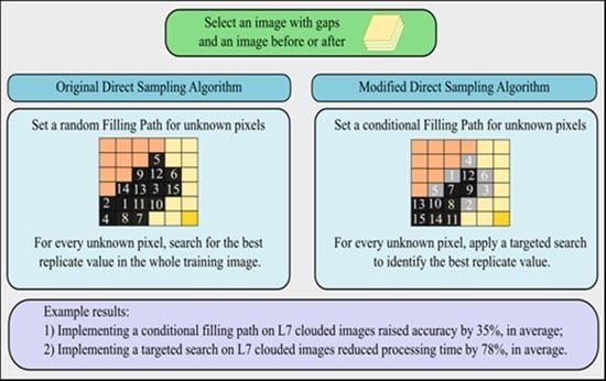
2.2.1. Modified Direct Sampling Method

Figure 2 shows the different steps associated with the application of the modified GF algorithm for a selected image band. The first proposed modification refers to applying a conditional filling path of UPs. In the original DS method, the user can define the filling path of UPs to be either random or unilateral. However, in both of these approaches, there is a good chance that the selected UP does not have any known neighbors, and therefore it will be assigned a random value. If this value is too different from the actual observation, it will negatively affect most of the subsequent iterations. To avoid such a situation, the present study suggests giving priority to UPs that have a specified number of known neighbors. This user-specified number is indicated as a new parameter “minNx”. The part of the algorithm that will search for a replicate will then run using the selected subset of UPs (with the order of items in the subset being random). At the end, the algorithm will update the target image with the new KP values and check again for UPs that satisfy the aforementioned condition. This operation will be repeated until no UP is identified in the target image. It is to be noted that assigning a value of zero to the parameter “minNx” means that the algorithm will behave as defined by the original DS method. The second proposed modification refers to applying a targeted search for the best replicate value to be assigned to the selected UP. Basically, instead of exhaustively searching the whole Training Image (TI), the search can be carried out on a specific portion of the TI. This portion is determined based on the following algorithmic steps: (i) The original list of KP coordinates in the TI is divided into a number of groups. The latter is defined by the user and is indicated as a new parameter “n2”; (ii) identifying each element in Nx corresponds to which group of KPs (generated with n2); and (iii) searching for the replicate pixel value in the identified groups instead of in all the training image. It should be noted that the user still maintains the ability to apply the fraction “f” parameter on the newly constructed list of KP coordinates. The fraction parameter allows the user to limit the search area to a user-defined fraction of the TI. For example, the search can be carried out on 80% of KPs in the TI, which will further speed up the simulations. It is to be noted that assigning a value of one to the parameter “n2” means that the algorithm will behave as defined by the original DS method.
For the present implementation of the DS method, two versions of the algorithm were prepared: one for a uni-layer (UL) simulation and the other for a bi-layer (BL) simulation. In the case of a UL simulation, the algorithm will use one training image (layer) to predict the UP values. This TI can either be the target image itself (if the number of UP values does not exceed that of KP values) or an image acquired before or after a specified window time. If more than one image is available during that period, the one containing the highest number of KP values will be selected. In the case of a BL simulation, the algorithm will use one training image (1st layer) and an auxiliary image (2nd layer) to predict the UP values. The TI will always be the target image, while the auxiliary image will correspond to an image acquired within a specified window time that happens to contain the smallest number of UP values. Similar to the work of Yin et al. [10], the pattern matching between Nx and Ny was assessed based on calculating the Euclidean distance equation described in their paper.

2.2.2. Experimental Setting

Three satellite imagery datasets (D1, D2, and D3) were prepared in the form of 450 × 450-pixel areas. For every dataset, one reference (gap-free) image was randomly selected, and from each one, a number of realistic simulations of gap-filled images were generated. This process is based on a random selection of SCL files with varying levels of gaps (Table 2). For every target image, the algorithm will additionally check the four closest images in time. Depending on the target image’s geographical location and whether it corresponds to L7 or S2, the temporal distance between two subsequent images may vary between 3 and 15 days. The acquisition dates of all the selected L7 and S2 images are listed in Table 3. The gap filling of satellite images was performed using two versions of the algorithm: Uni-layer and Bi-layer. The search for the best parameter combination was carried out by checking possible combinations that can be performed using the parameters’ values indicated in Table 2. In the end, the following unified parameter combination was adopted: n1 = 14; t = 0.01; f = 1; n2 = 200; minNx = 4; and (w1; w2) = (0.5; 0.5).

2.3. Performance Assessment

The evaluation of GF results was implemented for every artificially gap-filled image band. Five repetitions were performed to make sure that the effect of the randomness factor was negligible. Performance was assessed based on the following three error metrics: (i) mean square logarithmic error (MSLE), (ii) mean square error (MSE), and (iii) coefficient of determination (R2). In fact, the slope of the regression line provides an understanding of the under- or over-estimation of predicted versus actual values.
Their formulas are expressed below (where Pi indicates the predicted value, and Ai indicates the actual value):
MSLE = i = 1 N ( log 10 ( Pi ) log 10 ( Ai ) ) 2 N
MSLE is a modified version of the MSE that reflects the relative error between the estimated and actual values without giving importance to the error magnitude. It is usually adopted when the user does not want to penalize large individual errors that may occur.
MSE = i = 1 N ( Pi Ai ) 2 N
MSE is one of the most commonly used error metrics for quantifying loss. However, it can be significantly affected by outliers.
R 2 = ( i = 1 N ( Pi Pi ¯ ) ( Ai Ai ¯ ) i = 1 N ( Pi Pi ¯ ) 2 i = 1 N ( Ai Ai ¯ ) 2 ) 2
R2 is a widely adopted metric for assessing the consistency between estimated and actual observations. However, a few extreme errors can have a severe impact on this metric.

3. Results

As was mentioned before, two versions of the GF algorithm (UL and BL) were implemented on artificially created images (with every image containing either six or ten bands). Figure 3 reports R2 and processing time values corresponding to different gap percentages for two representative bands, namely B01 and B04. A complete list of all error metrics’ results for all investigated bands is presented in Annexes Tables S1–S3 (available in the Supplementary File). Figure 3a,b indicate that for D1 and D3, the accuracy values of applying either version of the GF algorithm range, respectively, from 52 to 96% and from 58 to 90%. The standard deviation between calculated R2 values is as follows: 4.5% (B01 in D1), 7.5% (B01 in D3), 0.9% (B04 in D1), and 7.6% (B04 in D3). By comparison, in the case of D2, accuracy values vary from 10 to 62% (B01) and from 66 to 92% (B04) (excluding P4-related results). The standard deviation of B01 and B04 in D2 are, respectively, estimated to be 21% and 13% (excluding P4-related results). On the other hand, Figure 3c,d show that the processing time for D1 and D3 ranges mostly between 1 and 8 min, whilst in the case of D2, running the simulation can take up to 30 min.
Results indicate that both the UL and BL algorithms are able to simulate realistic gap-filled images. As a matter of fact, the percentage of simulated bands with an accuracy value exceeding 70% is about 78% (UL algorithm) and 83% (BL algorithm). In addition, it is confirmed that the BL algorithm tends to outperform the UL algorithm in terms of accuracy. For example, in the case of B04 in D2 and a gap of 27.26%, accuracy values for UL and BL simulations are, respectively, 64.05 and 79.61%. However, this increase in accuracy seems to come at the cost of a longer processing time. Indeed, on average, the processing time needed to apply the BL algorithm is higher than that of the UL algorithm by around 232%. Moreover, the inspection of Annexes Tables S1–S3 reveals that in the case of D1 and D2, the least and most performing bands tend to be B01 and B04, respectively. By comparison, in the case of D3, it appears that there is no specific pattern to report. In general, for all three datasets, it is to be noted that most bands have a close performance between each other. In fact, for a selected gap percentage in any dataset, the accuracy values of at least two-thirds of all six (L7) or ten (S2) bands are within 5% of the average accuracy value of these bands. Furthermore, the GF algorithm seems to retain an acceptable performance irrespective of the spectral band type (L7 or S2) and the type of gaps (systematic sensor error or natural clouds). Exceptions in the form of simulations with very low accuracy values are largely attributed to the presence of patterns Nx that do not have enough similar matches Nys in the TI.
Generally speaking, L7 and S2 images that have been gap filled using the modified GF algorithm can retain a good overall accuracy and the general spatial characteristics of the different land cover types as long as a good number and distribution of similar patterns (associated with Nx) are available. Figure 4 and Figure 5 show some examples of L7 and S2 imagery (B04) before and after gap filling. Based on a visual inspection of these figures, the gap-filled images can be categorized into two cases. The first case corresponds to images with spread-out gaps, while the second case corresponds to images with dense gaps that tend to cover large swaths of land and/or sea. The GF algorithm tends to perform the best in the first case and vice versa. For example, although the L7 image (with a mask acquired on 19 April 2002) and the Sentinel 2 image (with a mask acquired on 22 August 2021) have very similar gap percentages (34.76 and 31.06%), they gave very different results when applying the GF algorithm. Indeed, as indicated in Figure 3b, the L7 accuracy results were even in the negative, while the S2 accuracy results ranged between 68 and 75% (depending on whether the UL or BL version of the algorithm was used). The negative results of the aforementioned L7 example are attributed to the fact that the reflectance values corresponding to the land surface were totally covered by clouds, and the only remaining known pixel values (that will be searched) correspond to water. One possible solution to mitigate this issue is to exclude the problematic pixels or delay their analysis till the end (so as to minimize the propagation of large erroneous estimations). Another possible solution is to fill the identified problematic pixels with another gap-filling approach (preferably one that is considered a temporal method). Identifying problematic pixels can be conducted by inspecting a gap-free image that is close in time.
Table 4 corresponds to the implementation of a UL algorithm on D2. The results of testing the other datasets (D1 and D3) are reported in Annexes Tables S4–S9 (available in the Supplementary File). Table 4 reveals a significant gain in processing time when implementing a targeted search for replicate values, and a clear improvement in overall accuracy can be seen after imposing a conditional filling path (where the algorithm starts with UP that has a user-specified minimum number of known neighbors). Indeed, the results derived from this study indicate that the average gain in processing time following the implementation of a targeted search (n2 = 200) is estimated to be 69.08% (D1), 78.18% (D2), and 90.77% (D3), while the average increase in accuracy following the implementation of a conditional filling path (minNx = 4) is estimated to be 1.73% (D1), 35.06% (D2), and 90.13% (D3). The indicated average values correspond to the average difference between implementing the proposed modification and the benchmark (original algorithm).

4. Discussion

Several research studies have focused on filling gaps in satellite imagery datasets. Identifying the most appropriate method among them usually depends on multiple factors, such as the processing time, the amount of data needed to generate reliable reconstructions of imagery, and whether or not the performance can be maintained consistently in different land cover settings and when applied on different spectral bands. The present work builds on the research conducted by Yin et al. [22]. The latter has demonstrated that the original gap-filling algorithm can reliably fill systematic gaps in L7 imagery in six land cover types that vary from being homogeneous to heterogeneous: (a) desert; (b) sparse agricultural; (c) dense farmland; (d) urban; (e) braided river; and (f) coastal areas. This is while requiring only one or two images as input data. In the present work, it has been confirmed that for coastal water bodies and when applying the modified GF algorithm to fill the systematic gaps, the achieved overall accuracy and processing time were better than those corresponding to the original algorithm. In addition, it was demonstrated that, as long as clouded pixels are spread out and do not totally cover a specific range of reflectance values, then the same performance can be achieved, whether using L7 or S2 imagery. Moreover, as evidenced in this work, using the BL version of the algorithm consists of trading a longer processing time for more accurate reconstructions of gap-filled images. Therefore, it is recommended to opt for mixing the use of the UL and BL versions based on the user’s specific needs.
The present modified DS algorithm was developed in a way to implement a CPU-based parallelization for the processing of images. However, according to the research conducted by [45], writing the code while implementing a GPU-based parallelization can lead to more significant gains in computational time. However, the latter method can be affected by several limitations, such as: (i) the financial costs of installing a graphics card, which is not always present in computers, and (ii) a larger memory demand. On the other hand, some temporal-based approaches were reported to produce similar satisfactory results to the DS algorithm. However, they tend to require a larger number of TIs, a higher memory demand for the storage of data, and a longer processing time. For instance, in the research study carried out by Alvera-Azcarate et al. [46] and Hilborn et al. [47], it was indicated that for the DINEOF method to achieve sufficiently good results, the authors needed to use three months of daily imagery. Similarly, the study of Sarafanov et al. [48] on the use of machine learning for filling gaps in land surface temperature, NDVI, and surface albedo remote sensing data gave good results, with the main drawbacks being the use of several hundreds of images for training purposes, and the need to developing customized models for every biome and/or land cover type.
An exhaustive comparison of the different variants of the DS method is difficult to carry out due to the fact that research studies were performed on various types and sizes of datasets. However, it is worth mentioning that the proposed two modifications can easily be incorporated into other variants of the DS method. For example, it is possible to combine the present algorithm with the bunch-pasting DS [18] and the tree-based DS [36]. The aforementioned algorithms were developed with the focus of reducing the computational costs of applying the DS approach on large imagery scenes. The bunch-pasting DS proposes pasting not only the replicate pixel value but also a user-defined number of its known neighbors at the same time. Defining a larger bunch size can significantly reduce the computational time but may result in a less accurate reproduction of patterns. The Tree-based DS introduces the concept of a clustering tree that is used for grouping similar patterns and their fast lookup. However, it requires that the TI does not have any gaps.

5. Conclusions

The presence of gaps in optical satellite imagery is a common problem that can limit the ability of agencies to continuously monitor the environment. The original Direct Sampling approach represents a widely used gap-filling algorithm that has been applied to various types of data. In this paper, two modifications to the original Direct Sampling approach are proposed, namely (i) a conditional filling path of unknown pixels and (ii) a targeted search of replicate values. It has been confirmed that the proposed two modifications have, indeed, helped in improving the simulation results and in speeding up the processing of images to the extent that the user can perform the analysis on his normal laptop without the need for purchasing special hardware. Results indicate that implementing either a UL or BL version of the GF algorithm produces mostly satisfactory gap-filled images, irrespective of the type of gaps and/or spectral band. Erroneous reconstructions of missing patterns tend to occur when a range of reflectance values is totally masked out in the TI. It is suggested that this problem can be mitigated or even eliminated by either (i) postponing the filling of problematic UPs until the end of the simulation or (ii) removing them from the analysis. In addition, it has been evidenced that although the BL version takes longer to compute simulations, it tends to largely outperform the UL version in terms of accuracy. Two possible directions for further research could be (i) to combine the modifications presented in this paper with other variants of the DS algorithm as a way to further speed up the processing and (ii) to experiment with more types of auxiliary images in the BL version as a way to automatically identify problematic pixels from the start.

Supplementary Materials

The following supporting information can be downloaded at: https://www.mdpi.com/article/10.3390/rs15215122/s1.

Author Contributions

Conceptualization, L.F., I.M., G.S. and C.K.; Data curation, L.F.; Formal analysis, L.F.; Funding acquisition, I.M., G.S. and C.K.; Investigation, L.F.; Methodology, L.F., I.M., G.S. and C.K.; Project administration, L.F. and C.K.; Resources, L.F., I.M. and G.S.; Software, L.F.; Supervision, I.M., G.S. and C.K.; Validation, L.F.; Visualization, L.F. and I.M.; Writing—original draft, L.F.; Writing—review and editing, L.F., I.M., G.S. and C.K. All authors have read and agreed to the published version of the manuscript.

Funding

This research has received funding from: (a) the ESA Mediterranean Regional Initiative Applications–Theme 2 ‘SEA’-Segment1 ESA programmatic line (2020–2022): MEDEOS Contract MIR-DMS-COM-PRS01-E under the reference AO/1-10376/20/I-EF, and (b) Erasmus+ Programme: Knowledge Alliances TERRATECH–masTERs course on smArt Agriculture TECHnologies, Project Number: 621568-EPP-1-2020-1-PT-EPPKA2-KA.

Data Availability Statement

Data acquisition has been explained in the methodology section. The corresponding code repository has been published under an MIT open License “https://github.com/farhatlokmen/GapFilling.jl (accessed on 23 October 2023)”.

Conflicts of Interest

The authors declare that they have no known competing financial interests or personal relationships that could have appeared to influence the work reported in this paper.

References

  1. Banskota, A.; Kayastha, N.; Falkowski, M.J.; Wulder, M.A.; Robert, E.; White, J.C. Forest Monitoring Using Landsat Time Series Data: A Review. Can. J. Remote Sens. 2014, 40, 362–384. [Google Scholar] [CrossRef]
  2. Jamshidi, S.; Zand-parsa, S.; Niyogi, D. Assessing Crop Water Stress Index of Citrus Using In-Situ Measurements, Landsat, and Sentinel-2 Data. Int. J. Remote Sens. 2021, 42, 1893–1916. [Google Scholar] [CrossRef]
  3. Du, Y.; Song, K.; Liu, G.; Wen, Z.; Fang, C.; Shang, Y.; Zhao, F.; Wang, Q.; Du, J.; Zhang, B. Quantifying total suspended matter (TSM) in waters using Landsat images during 1984–2018 across the Songnen Plain, Northeast China. J. Environ. Manag. 2020, 262, 110334. [Google Scholar] [CrossRef]
  4. Jamshidi, S.; Zand-parsa, S.; Pakparvar, M.; Niyogi, D. Evaluation of Evapotranspiration over a Semi-Arid Region using Multi-Resolution Data Sources. J. Hydrometeorol. 2019, 20, 947–964. [Google Scholar] [CrossRef]
  5. Naghdyzadegan Jahromi, M.; Zand-parsa, S.; Razzaghi, F.; Jamshidi, S.; Didari, S.; Doosthosseini, A.; Reza Pourghasemi, H. Developing machine learning models for wheat yield prediction using ground-based data, satellite-based actual evapotranspiration and vegetation indices. Eur. J. Agron. 2023, 146, 126820. [Google Scholar] [CrossRef]
  6. Bannari, A.; Al-ali, Z.M. Assessing Climate Change Impact on Soil Salinity Dynamics between 1987–2017 in Arid Landscape Using Landsat TM, ETM+ and OLI Data. Remote Sens. 2020, 12, 2794. [Google Scholar] [CrossRef]
  7. Cammarano, D.; Jamshidi, S.; Hoogenboom, G.; Ruane, A.C.; Niyogi, D.; Ronga, D. Processing tomato production is expected to decrease by 2050 due to the projected increase in temperature. Nat. Food 2022, 3, 437–444. [Google Scholar] [CrossRef]
  8. Amani, M.; Member, S.; Ghorbanian, A.; Ahmadi, S.A.; Moghimi, A.; Mirmazloumi, S.M.; Member, S.; Hamed, S.; Moghaddam, A.; Mahdavi, S.; et al. Google Earth Engine Cloud Computing Platform for Remote Sensing Big Data Applications: A Comprehensive Review. IEEE J. Sel. Top. Appl. Earth Obs. Remote Sens. 2020, 13, 5326–5350. [Google Scholar] [CrossRef]
  9. Shao, Z.; Fu, H.; Li, D.; Altan, O.; Cheng, T. Remote sensing monitoring of multi-scale watersheds impermeability for urban hydrological evaluation. Remote Sens. Environ. 2019, 232, 111338. [Google Scholar] [CrossRef]
  10. Weiss, D.J.; Atkinson, P.M.; Bhatt, S.; Mappin, B.; Hay, S.I.; Gething, P.W. An effective approach for gap-filling continental scale remotely sensed time-series. ISPRS J. Photogramm. Remote Sens. 2014, 98, 106–118. [Google Scholar] [CrossRef]
  11. Belda, S.; Pipia, L.; Morcillo-pallarés, P.; Rivera-caicedo, J.P.; Amin, E.; De Grave, C.; Verrelst, J. Europe PMC Funders Group DATimeS: A machine learning time series GUI toolbox for gap-filling and vegetation phenology trends detection. Environ. Model. Softw. 2022, 127, 104666. [Google Scholar] [CrossRef]
  12. Freyr, A.; Baum, A.; Vicente-serrano, S.M.; Stockmarr, A. Gap-Filling of NDVI Satellite Data Using Tucker Decomposition: Exploiting Spatio-Temporal Patterns. Remote Sens. 2021, 13, 4007. [Google Scholar]
  13. Li, M.; Zhu, X.; Li, N.; Pan, Y. Gap-Filling of a MODIS Normalized Difference Snow Index Product Based on the Similar Pixel Selecting Algorithm: A Case Study on the Qinghai–Tibetan Plateau. Remote Sens. 2020, 12, 1077. [Google Scholar] [CrossRef]
  14. Chen, J.; Zhu, X.; Vogelmann, J.E.; Gao, F.; Jin, S. A simple and effective method for filling gaps in Landsat ETM + SLC-off images. Remote Sens. Environ. 2011, 115, 1053–1064. [Google Scholar] [CrossRef]
  15. Kandasamy, S.; Baret, F.; Verger, A.; Neveux, P.; Weiss, M. A comparison of methods for smoothing and gap filling time series of remote sensing observations–application to MODIS LAI products. Biogeosciences 2013, 10, 4055–4071. [Google Scholar] [CrossRef]
  16. Henn, B.; Raleigh, M.S.; Fisher, A.; Lundquist, J.D. A Comparison of Methods for Filling Gaps in Hourly Near-Surface Air Temperature Data. Am. Meteorol. Soc. 2013, 14, 929–945. [Google Scholar] [CrossRef]
  17. Noor, N.M.; Mustafa, M.; Bakri, A.; Yahaya, A.S.; Ramli, N.A. Comparison of Linear Interpolation Method and Mean Method to Replace the Missing Values in Environmental Data Set. Mater. Sci. Forum 2015, 803, 278–281. [Google Scholar] [CrossRef]
  18. Rezaee, H.; Mariethoz, G.; Koneshloo, M.; Asghari, O. Multiple-point geostatistical simulation using the bunch-pasting direct sampling method. Comput. Geosci. 2013, 54, 293–308. [Google Scholar] [CrossRef]
  19. Aitokhuehi, I.; Durlofsky, L.J. Optimizing the performance of smart wells in complex reservoirs using continuously updated geological models. J. Pet. Sci. Eng. 2005, 48, 254–264. [Google Scholar] [CrossRef]
  20. Hoffman, B.T.; Caers, J. History matching by jointly perturbing local facies proportions and their spatial distribution: Application to a North Sea reservoir. J. Pet. Sci. Eng. 2007, 57, 257–272. [Google Scholar] [CrossRef]
  21. Huysmans, M.; Dassargues, A. Application of multiple-point geostatistics on modelling groundwater flow and transport in a cross-bedded aquifer (Belgium). Hydrogeol. J. 2009, 17, 1901–1911. [Google Scholar] [CrossRef]
  22. Yin, G.; Mariethoz, G.; McCabe, M.F. Gap-filling of landsat 7 imagery using the direct sampling method. Remote Sens. 2017, 9, 12. [Google Scholar] [CrossRef]
  23. Guardiano, F.B.; Srivastava, R.M. Multivariate Geostatistics: Beyond Bivariate Moments; Springer: Dordrecht, The Netherlands, 1993. [Google Scholar]
  24. Strebelle, S. Conditional Simulation of Complex Geological Structures Using Multiple-Point Statistics 1. Math. Geol. 2002, 34, 1–21. [Google Scholar] [CrossRef]
  25. Zhang, T.; Switzer, P.; Journel, A. Filter-Based Classification of Training Image Patterns for Spatial Simulation. Int. Assoc. Math. Geol. 2006, 38, 62–80. [Google Scholar] [CrossRef]
  26. Gloaguen, E.; Dimitrakopoulos, R. Two-dimensional Conditional Simulations Based on the Wavelet Decomposition of Training Images. Math. Geosci. 2009, 41, 679–701. [Google Scholar] [CrossRef]
  27. Honarkhah, M.; Caers, J. Stochastic Simulation of Patterns Using Distance-Based Pattern Modeling Distance-based Method. Math. Geosci. 2010, 42, 487–517. [Google Scholar] [CrossRef]
  28. Tahmasebi, P.; Hezarkhani, A.; Sahimi, M. Multiple-point geostatistical modeling based on the cross-correlation functions. Comput. Geosci. 2012, 16, 779–797. [Google Scholar] [CrossRef]
  29. Straubhaar, J.; Renard, P.; Mariethoz, G.; Froidevaux, R.; Besson, O. An Improved Parallel Multiple-point Algorithm Using a List Approach. Math. Geosci. 2011, 43, 305–328. [Google Scholar] [CrossRef]
  30. Straubhaar, J.; Walgenwitz, A.; Renard, P. Parallel Multiple-Point Statistics Algorithm Based on List and Tree Structures. Math. Geosci. 2013, 45, 131–147. [Google Scholar] [CrossRef]
  31. Mariethoz, G.; Renard, P. Reconstruction of Incomplete Data Sets or Images Using Direct Sampling. Math. Geosci. 2010, 42, 245–268. [Google Scholar] [CrossRef]
  32. Abdollahifard, M.J.; Faez, K. Fast direct sampling for multiple-point stochastic simulation. Arab. J. Geosci. 2013, 15, 1927–1939. [Google Scholar] [CrossRef]
  33. Feng, W.; Wu, S.; Yin, Y.; Zhang, J.; Zhang, K. A training image evaluation and selection method based on minimum data event distance for multiple-point geostatistics. Comput. Geosci. 2017, 104, 35–53. [Google Scholar] [CrossRef]
  34. Zuo, C.; Pan, Z.; Gao, Z.; Gao, J. Correlation-driven direct sampling method for geostatistical simulation. Am. Phys. Soc. 2019, 99, 053310. [Google Scholar] [CrossRef]
  35. Soltan Mohammadi, H.; Javad Abdollahifard, M.; Doulati Ardejani, F. CHDS: Conflict handling in direct sampling for stochastic simulation of spatial variables. Stoch. Environ. Res. Risk Assess. 2020, 4, 23. [Google Scholar] [CrossRef]
  36. Zuo, C.; Yin, Z.; Pan, Z.; Mackie, E.J.; Jef, C. A Tree-Based Direct Sampling Method for Stochastic Surface and Subsurface Hydrological Modeling. Water Resour. Res. 2020, 56, 20. [Google Scholar] [CrossRef]
  37. Antonelli, C.; Eyrolle, F.; Rolland, B.; Provansal, M.; Sabatier, F. Suspended sediment and 137Cs fluxes during the exceptional December 2003 flood in the Rhone River, southeast France. Geomorphology 2008, 95, 350–360. [Google Scholar] [CrossRef]
  38. Delile, H.; Masson, M.; Miège, C.; Le Coz, J.; Poulier, G.; Le Bescond, C.; Radakovitch, O.; Coquery, M. Hydro-climatic drivers of land-based organic and inorganic particulate micropollutant fluxes: The regime of the largest river water inflow of the Mediterranean Sea. Water Res. 2020, 185, 116067. [Google Scholar] [CrossRef] [PubMed]
  39. Comby, E.; Le Lay, Y.F.; Piégay, H. How chemical pollution becomes a social problem. Risk communication and assessment through regional newspapers during the management of PCB pollutions of the Rhône River (France). Sci. Total Environ. 2014, 482, 100–115. [Google Scholar] [CrossRef] [PubMed]
  40. Ludwig, W.; Meybeck, M. Riverine Transport of Water, Sediments and Pollutants to the Mediterranean Sea, UNEP/MAP/MED POL, MAP Technical Reports Series; No. 141; UNEP/MAP: Athens, Greece, 2003. [Google Scholar]
  41. UNESCO Parc Naturel Régional de Camargue. Available online: https://en.unesco.org/biosphere/eu-na/camargue (accessed on 23 October 2023).
  42. Mariethoz, G.; Renard, P.; Straubhaar, J. The direct sampling method to perform multiple-point geostatistical simulations. Water Resour. Res. 2010, 46, 1–14. [Google Scholar] [CrossRef]
  43. Meerschman, E.; Pirot, G.; Mariethoz, G.; Straubhaar, J.; Van Meirvenne, M.; Renard, P. A practical guide to performing multiple-point statistical simulations with the Direct Sampling algorithm. Comput. Geosci. 2013, 52, 307–324. [Google Scholar] [CrossRef]
  44. Farhat, L. A Set of Algorithms for Preprocessing and Gap Filling of Landsat 7 and Sentinel 2 Imagery Using a Modified Direct Sampling Approach. Available online: https://github.com/farhatlokmen/GapFilling.jl (accessed on 23 October 2023).
  45. Huang, T.; Li, X.; Zhang, T.; Lu, D. GPU-accelerated Direct Sampling method for multiple-point statistical simulation. Comput. Geosci. 2013, 57, 13–23. [Google Scholar] [CrossRef]
  46. Alvera-Azcárate, A.; Barth, A.; Beckers, J.M.; Weisberg, R.H. Multivariate reconstruction of missing data in sea surface temperature, chlorophyll, and wind satellite fields. J. Geophys. Res. 2007, 112, 1–11. [Google Scholar] [CrossRef]
  47. Hilborn, A.; Costa, M. Applications of DINEOF to Satellite-Derived Chlorophyll-a from a Productive Coastal Region. Remote Sens. 2018, 10, 1449. [Google Scholar] [CrossRef]
  48. Sarafanov, M.; Kazakov, E.; Nikitin, N.O.; Kalyuzhnaya, A.V. A Machine Learning Approach for Remote Sensing Data Gap-Filling with Open-Source Implementation: An Example Regarding Land Surface Temperature, Surface Albedo and NDVI. Remote Sens. 2020, 12, 3865. [Google Scholar] [CrossRef]
Figure 1. (a) Location of the study area and (b) a Landsat 7 image depicting the study area with systematic gaps and a cloudy condition.
Remotesensing 15 05122 g001
Figure 2. Workflow of the gap-filling algorithm (Black text refers to steps that did not change; red text refers to steps that were deprecated in the modified version; green text refers to implemented modifications) (Nx: Known pixels that are neighbors of the selected unknown pixel).
Remotesensing 15 05122 g002
Figure 3. Accuracy values (R2: y-axis) for B01 (a) and B04 (b) and processing time (seconds: y-axis) for B01 (c) and B04 (d); (D1: L7 images with systematic gaps, D2: L7 images with cloud gaps, D3: S2 images with cloud gaps).
Remotesensing 15 05122 g003
Figure 4. Landsat 7 (band B04) images before and after gap filling with the uni-layer version of the algorithm.
Remotesensing 15 05122 g004
Figure 5. Sentinel 2 (band B04) images before and after gap filling with the uni-layer version of the algorithm.
Remotesensing 15 05122 g005
Table 1. Landsat 7 (L7) and Sentinel 2 (S2) band designation and characteristics.
Imagery SeriesSpectral Band DesignationDescriptionCentral
Wavelength (nm)
Resolution (m)
L7B01Blue450–52030
B02Green520–60030
B03Red630–69030
B04Near Infrared770–90030
B05Shortwave Infrared1550–175030
B07Shortwave Infrared2080–235030
S2B02Blue433–45310
B03Green458–52310
B04Red543–57810
B05Vegetation Red Edge650–68020
B06Vegetation Red Edge698–71320
B07Vegetation Red Edge733–74820
B08Near Infrared (NIR)785–90010
B8ANear NIR855–87520
B11Shortwave Infrared1565–165520
B12Shortwave Infrared2100–228020
Table 2. Acquisition dates and gap percentage of used satellite images.
D1D2D3
DateGap (%)DateGap (%)DateGap (%)
200101260200101260202103280
2005120710.702002041934.76202107263.19
200512238.94 (P1)200204281002021072812.47 (P1)
200506309.962002050511.79 (P1)2021073151.51
2005071614.23 (P2)200205141002021102181.86
2005080166.94200205210.122021102418.57 (P2)
2002011319.25202110260.48
2002012915.93 (P2)202102212.71
200203182.52021022326.63 (P3)
20030201020210226100
2003021727.26 (P3)202108200.22
200303050.052021082231.06 (P4)
200203182.520210825100
2002041934.76 (P4)
20020428100
Dates written in italics correspond to reference images; Dates written in bold correspond to target images; Other dates correspond to images acquired before or after target images; P1 to P4: abbreviations to gap percentages to be used in subsequent figures.
Table 3. Parameter values that were investigated to achieve the best gap-filling results.
ParameterCases
n18–14–20–24
n21–50–100–150–200
t0.005–0.007–0.01
f1
minNx0–2–4–6
(w1; w2)(0.25; 0.75)–(0.5; 0.5)–(0.75; 0.25)
n1: Number of neighbors to be checked for a selected UP; n2: Number of groups into which the KPs of the TI will be divided; t: Distance threshold; f: Search fraction; minNx: minimum number of known neighbors to be enforced for a selected UP; w1/w2: Weight values corresponding to target image (BL algorithm) (Their sum should be equal to 1).
Table 4. Reduction in (a) processing time (%) when applying a targeted search for the best replicate in D2 and (b) overall accuracy (%) when imposing a conditional filling path in D2 (n2: Number of groups into which the KPs of the TI will be divided; minNx: minimum number of known neighbors to be enforced for a selected UP; minNx = 0 is the benchmark; Simulations were performed using the uni-layer algorithm).
(a)
Overall Accuracy (%) When Imposing a Conditional
Filling Path
(b)
Processing Time (%) When
Applying a Targeted Search
n2minNx
Gap (%)Band501001502000246
11.8B0162.9577.6082.0387.56−17.78−1.3210.685.48
B0278.3986.6590.0491.10−10.6522.2334.7227.42
B0368.9978.5984.4485.66−4.9534.641.0939.19
B0482.7588.3589.8688.96−7.4167.0768.2368.43
B0582.2084.9285.7385.19−5.9350.8859.8855.99
B0765.1675.3880.1179.78−6.8747.4649.1352.73
15.94B0146.5462.0269.8178.1935.9357.5458.9458.04
B0255.7167.4370.1780.5254.0377.8378.5378.27
B0340.9353.3661.2970.6359.1679.4180.6681.47
B0457.4161.8865.1274.6970.0193.7193.9594.35
B0544.0250.3652.0351.9164.5287.6787.8388.12
B0734.4041.9542.6441.9559.9780.9181.1181.01
27.26B0155.7472.0279.3386.25−3.1618.8514.4412.84
B0268.3280.5883.2488.760.4342.5443.438.23
B0356.2868.3775.0181.740.6749.147.246.7
B0475.1980.7886.3783.54−6.7461.3564.0164.03
B0558.9665.1168.5268.81−5.347.3943.8744.55
B0751.4960.9360.0460.26−4.540.838.8238.74
34.76B0175.3389.6192.0793.76−27.7−12.94−12.69−10.01
B0275.3784.5288.7292.17−30.52−18.69−19.51−17.81
B0360.9775.1481.8986.43−26.67−22.84−20.79−22.3
B0439.9665.8368.3476.45−33.56−31.86−29.97−29.46
B0516.6325.5439.0144.75−28.09−26.34−25.4−26.41
B0743.4139.0840.4144.12−25.52−25.99−25.42−24.62
Disclaimer/Publisher’s Note: The statements, opinions and data contained in all publications are solely those of the individual author(s) and contributor(s) and not of MDPI and/or the editor(s). MDPI and/or the editor(s) disclaim responsibility for any injury to people or property resulting from any ideas, methods, instructions or products referred to in the content.

