
Crustal Imaging across the Princess Elizabeth Land, East Antarctica from 2D Gravity and Magnetic Inversions
by
 ,
,
Lin Li
1,†, 
Enzhao Xiao
1,
Xiaolong Wei
2,†,
Ning Qiu
3,*,
Khalid Latif
4,
Jingxue Guo
1 and
Bo Sun
1 1
Polar Research Institute of China, Shanghai 200136, China
2
Department of Earth & Atmospheric Sciences, University of Houston, Houston, TX 77204, USA
3
South China Sea Institute of Oceanology, Chinese Academy of Sciences, Guangzhou 510301, China
4
National Centre of Excellence in Geology, University of Peshawar, Peshawar 25130, Pakistan
*
Author to whom correspondence should be addressed.
†
These authors contributed equally to this work.
Remote Sens. 2023, 15(23), 5523; https://doi.org/10.3390/rs15235523
Submission received: 28 September 2023
/
Revised: 10 November 2023
/
Accepted: 14 November 2023
/
Published: 27 November 2023
(This article belongs to the Special Issue Geographic Data Analysis and Modeling in Remote Sensing)
Abstract
:The Princess Elizabeth Land landscape in East Antarctica was shaped by a complex process, involving the supercontinent’s breakup and convergence cycle. However, the lack of geological knowledge about the subglacial bedrock has made it challenging to understand this process. Our study aimed to investigate the structural characteristics of the subglacial bedrock in the Mount Brown region, utilizing airborne geophysical data collected from the China Antarctic Scientific Expedition in 2015–2017. We reconstructed bedrock density contrast and magnetic susceptibility models by leveraging Tikhonov regularized gravity and magnetic inversions. The deep bedrock in the inland direction exhibited different physical properties, indicating the presence of distinct basement sources. The east–west discontinuity of bedrock changed in the inland areas, suggesting the possibility of large fault structures or amalgamation belts. We also identified several normal faults in the western sedimentary basin, intersected by the southwest section of these survey lines. Furthermore, lithologic separators and sinistral strike-slip faults may exist in the northeast section, demarcating the boundary between Princess Elizabeth Land and Knox Valley. Our study provides new insights into the subglacial geological structure in this region, highlighting the violent impact of the I-A-A-S (Indo-Australo-Antarctic Suture) on the subglacial basement composition. Additionally, by identifying and describing different bedrock types, our study redefines the potential contribution of this region to the paleocontinent splicing process and East Antarctic basement remodeling.
1. Introduction
The East Antarctica Ice Sheet (EAIS) covers a continent that remains poorly understood in terms of its topography and geology [1,2]. A complex tectonic evolution history was formed by the supercontinent process, including the composite shield dominated by Columbia and Rodinia in the Precambrian era [3,4,5,6,7,8,9], as well as the convergence and fragmentation of Gondwana [10,11,12]. Research data deficiencies and the complexity of the causal mechanisms have hindered the knowledge of the basement characteristics and splicing position of the suture belt in this region, making it a research focus under the EAIS. However, after an aero-geophysical survey that covered other areas of East Antarctica, such as Queen Maud Land, Enderby Land, William II Land, and Wilkes Land, the suture belts in these areas, which were closely related to Africa and Australia in the Gondwana period, have been gradually revealed [2,10,13,14,15,16,17]. It has become generally recognized that the tectonic domain related to India Plate is located in the Indian Ocean sector of Antarctica, and possible suture belts extend from Alasheyev Bight in Enderby Land to the Denman Glacier in Queen Mary Land [18,19,20]. Bedrock exposures are concentrated in the western part of this domain, including the Napier-Tula-Scott Mountains, the Prince Charles Mountains (PCM), and Prydz Bay. In contrast, the existence of ice sheets and only the exposure of Mount Brown in the eastern region limit the geological cognition of sutures belts in the inland direction [18,19,21,22]. Considering that the tectonic units in this area include the results of multi-stage orogeny from the late Mesoproterozoic to the Early Cambrian [12,18,23], we believe that information about the bedrock under the ice sheet of this region could provide essential clues for the study of the tectonic intersection area between India and East Antarctica.
Our research area was located at the junction of Princess Elizabeth Land and William II Land, which is situated in the inland extension of the West ice shelf. The region of interest spans from the King Leopold and Queen Astrid Coast to the vicinity of Mount Brown, as depicted in Figure 1. The majority of the bedrock in this area is concealed by ice sheets, with outcrop areas being restricted to the Svenner Islands-Brattstr and Bluffs-Larsemann Hills, constituting 70 km long coastal outcrops of Prydz Bay [20] and Mount Brown, which is slightly higher than the inland ice sheet [19]. Gravity and magnetic data have wide applications in crustal imaging, mineral prospecting, and engineering and environmental studies [24,25,26]. In our work, we utilized the International Collaborative Exploration of Central East Antarctica through Airborne Geophysical Profiling (ICECAP) data, acquired by the China Antarctic Scientific Survey using the Snow Eagle 601 airborne geophysical survey platform in 2015–2017 [27]. The ICECAP data comprise an airborne high-performance ice radar system (HiCARS), GT-2A airborne gravimeter, and CS-3 magnetometer data. The ice radar data were used to calculate the surface elevation, ice sheet thickness, and bedrock elevation in the study area (Figure 2b–d), to improve the reliability of gravity data inversion. We calculated the gravity and magnetic anomalies of the bedrock using airborne gravity and magnetic data. We performed 2D Tikhonov regularized gravity and magnetic inversions [28,29] to obtain density contrast and magnetic susceptibility models of the subglacial bedrock for the four aerogeophysical survey profiles (Figure 2). To interpret the recovered models and identify geological units, we utilized outcrop petrology research findings and the tectonic evolution history of East Antarctica to enhance the reliability of the interpretation of the geophysical data results and provide valuable insights for exploring the bedrock characteristics of this complex subglacial mountain–rift system [10,19,20,21].
2. Geophysical Data Setting
2.1. Field Data Collection
The methods used to process the data were modified from industry-standard protocols, with full details provided in the data release notes. Geophysical data were acquired using the Snow Eagle 601 aero-geophysical platform and a BT-67 airplane operated by the Polar Research Institute of China as part of the Chinese National Antarctic Research Expedition (CHINARE) program during 2015–2017. The airplane was equipped with a suite of instruments, including an airborne high-performance ice radar system (HiCARS), a GT-2A airborne gravimeter, and a CS-3 magnetometer.
The HiCARS system is a frequency modulated phase coherent radar composed of digital control and recording subsystems, transmitters, receivers, and antennas. The system emits 6250 pulses per second, with the energy generated by a PXI digital controller with a frequency of 200 MHz and connected to an 8 kW Tomco amplifier. The center frequency of 60 MHz allows the detection of important glaciers and geological features. Signal superposition, pulse compression, sharpening filtering, signal focusing, and other methods are subsequently used to obtain more accurate and clear images of ice radar data. The system’s 15 MHz bandwidth pulse compression provides a depth resolution in the ice sheet of 10 to 15 m.
The GT-2A airborne gravimeter is a three-axis stable scalar gravimeter deployed on the Snow Eagle fixed-wing aircraft. The accelerometer maintains the vertical state and stability of the instrument, and the high-sensitivity acceleration measurement eliminates the acceleration caused by the movement of the aircraft. The GT-2A allows for operation in high latitude polar regions, with JAVAD Delta dual-frequency and carrier phase GNSS receivers used to connect GPS antennas and the GT-2A system at various positions on the aircraft, including the two wings, the front, and center of the fuselage, with an accuracy of 25 cm under normal circumstances.
The CS-3 magnetometer measures the magnetic field of the bedrock under the ice sheet and is installed on the tail of the Snow Eagle fixed-wing aircraft to avoid magnetic interference from the metal fuselage. The CS-3 magnetometer has a high sensitivity and low noise interference. During measurement, the CS-3 magnetometer measures an integrated response from deep and shallow structures, with the AARC510 providing compensation for the influence of flight direction and altitude.
The airborne platform was flown around 600 m above the ice surface with a speed of about 300 km/h. The rate of gravity data acquisition was 2 Hz. Free-air gravity anomaly was filtered with a 150 s full-wavelength low-pass filter to suppress the noise, with a resolution of 6.25 km along the track. The estimated error of the output free-air gravity signal was 1 mGal. In the data processing, we interpolated the data using the minimum curvature method. We corrected the free-air gravity data with density values of 2.67 g/cm for bedrock and 0.915 g/cm for ice layers. The resulting Bouguer gravity data were then used for gravity inversions.
2.2. Geophysical Inversion
Inversion, as a geophysical data interpretation method, aims to reconstruct subsurface physical property models. A commonly adopted objective function of inversion is [29,30,31]
where and indicate the data misfit term and the regularization term, respectively. is the regularization parameter.
Assuming the data noise follows an independent Gaussian distribution, the data misfit term can be defined as follows:
where is the estimated error for the ith datum. is the predicted data, is the observed data, and N is the amount of observation data. Similarly to the work of Li and Oldenburg [29], our regularization term consisted of four components, as shown below:
where the functions f are defined as follows:
the smallness component, , measures the size of a model m, and the other three components, , , and , measure the smoothness of the model features along the three orthogonal coordinate directions (x, y, z) in 3D. Weighting parameters (, , , ) control the contribution of each component and partly determine the characteristics of the features in an inverted model. Note that norm regularization [32,33], in contrast to norm regularization, produces compact models with clearly defined boundaries.
In our work, we performed gravity and magnetic inversions separately, to recovery the density contrast and susceptibility models. We used uniform initial models with zero density contrast and susceptibility value. For ice layers, we imposed zero density contrast and susceptibility values as constraints during the inversions. We also added padding cells, extending the maximum depth to 27,000 m, to account for the part of the signals from crust (i.e., long wavelength) and surrounding bedrock outside our survey lines. All inversions were performed using an open-source framework SimPEG [34,35], where the beta-cooling strategy was employed to find the appropriate regularization parameter.
3. Geophysical and Geological Interpretation
Following the construction of the relative density contrast and magnetic susceptibility models of the four profiles, various density contrast and magnetic susceptibility values were employed to differentiate the distinct lithologic units. Our analysis results demonstrated a certain degree of consistency between the density contrast and susceptibility models, indicating the reliability of our findings. Note that the positive and negative density contrast values show that the density of materials was higher or lower, respectively, than the background density, i.e., 2.67 g/cm. The recovered density contrast (Figure 3b) and susceptibility (Figure 3d) models revealed subsurface structures beneath survey line 1 (Figure 1). We divided the inverted density contrast model (Figure 3b) and susceptibility (Figure 3d) model into three zones. Zone A features low-density contrast and high susceptibility. It is likely to be mafic bedrocks. Zone B is characterized by high-density contrast and low susceptibility. There is an obvious low-density longitudinal consistency area in the middle of the line, and the transverse gradient changes greatly, the longitudinal extension is deeper, corresponding to the susceptibility close to the 0 value, we thus considered this point as corresponding to a deep fault.Zone C is an ice layer with zero density contrast and susceptibility.
In Figure 4b,d, we present the density contrast and susceptibility model recovered from survey line 2. This survey line was an extension of survey line 1 into the inland region (Figure 1). The recovered lithologic units of survey line 1 and survey line 2 showed a clear correlation, but the spatial distribution of these units changed noticeably. A distinct change in lithology is observed corresponding to survey line 1, which appears to be associated with the segmentation or splicing of different lithologic units dominated by fault structures (Figure 4b,d).
The recovered density contrast (Figure 5b) and susceptibility (Figure 5d) models exhibited a high degree of structural similarity. Zone D was characterized by intermediate negative density contrast and susceptibility features. Mishra et al. (1999) suggested that granitic plutons are associated with intermediate negative susceptibility and near-zero density contrast values, while silicic plutons are commonly characterized by a relatively low susceptibility and negative density contrasts.Therefore, we interpreted zone D as a mixture of granitic and silicic plutons. In zone B, the structures extend from the near-surface to deep depths, likely due to survey line 3 crossing the peaking area around Mount Brown (Figure 1), which is covered by a thin ice sheet. Considering the consistency of the physical properties of outcrop and subglacial bedrock, we suggested that the bedrock in this area is dominated by felsic orthogneisses with subordinate amounts of mafic granulites, anatectic paragneisses, and pegmatite veins [19]. The mountain-shaped bedrocks in zone A exhibited spatial continuity with zone A in line 2 (Figure 4b,d) and were interpreted as magmatic rocks and metamorphic rocks [20,21].
In survey line 4, we observed a distinct feature in the recovered models, namely a large area of deep negative susceptibility (Zone B and D in Figure 6d). Further analysis revealed that this negative susceptibility feature is comprised of two distinct geological units (Zones B, and D in Figure 6b) with different density contrasts. Zone D in Figure 6b corresponds to Zone D in Figure 5b, which we interpreted as a mixture of granitic and silicic plutons. Zone B exhibited a high positive density contrast and negative susceptibility values (with a maximum negative susceptibility at about −0.12 SI), suggesting that they could still be bedrock, possibly ultramafic, but with inverted magnetic polarities. We posited that the subsurface structures depicted in Figure 3, Figure 4, Figure 5 and Figure 6 were formed during different geological periods, reflecting the evolution of the study area into a stable inland terrane, possibly the East Antarctic craton [12,20,21]. Eight more aeromagnetic observations were conducted in this area in 2017. Combined with newly measured aeromagnetic data and ADMAP2 data [36], the fault locations were divided, as shown in Figure 7.
4. Discussion
4.1. Transilience of Physical Properties in Deep Bedrock
Our analysis of the bedrock structure included a focus on the development of high-density contrast characteristic bedrock units from the surface to the deep. These units exhibited obvious segmentation characteristics in their density contrast models, with the vertical change being much smaller than the horizontal change. In particular, the east–west distribution and spatial spacing of these units were interpreted as resulting from the tectonic dominant faults in the receiving area, with the surface structure of the subglacial bedrock reflecting the distribution of rifts and gullies.
We also observed a sharp change in the physical properties of the deep bedrock along certain survey lines. Specifically, from survey line 1 to survey line 4, there was an obvious north–south boundary of bedrock physical properties at the east side of Mount Brown, located between unit A and unit B from survey line 2 to survey line 4. This mutation is consistent with the bedrock structure identification of the tectonic development and erosion of the subglacial sedimentary basin in the south pole [2,37].
We also found that the continuity of high-density contrast models and the discontinuity of magnetic susceptibility changed in the hidden mountains in the Mount Brown area, suggesting a change in lithology. This change was found in the continuity of high-density contrast models in unit B from line 2 to line 4, while the magnetic susceptibility changed significantly between line 3 and line 4. This change in physical properties reflects the change in lithology, which has previously been identified in exposed samples of the Mount Brown area as felsic orthogneisses with subordinate amounts of mafic granulites, anatectic paragneisses, and pegmatite veins.
From a spatial distribution perspective, unit B in survey lines 3–4 was related to the change in physical properties of bedrock in the west, showing obvious physical properties cutting into the four survey lines, with the coordinate position as the boundary. This origin is consistent with the eastward extension of the Renna complex group identified through outcrop petrology.
Unit B in line 3 belongs to the Grenvillian product of long-term ocean subduction accretion from 1500–1000 Ma to the final collision at 1000–900 Ma, which is much earlier than the age of the formation of the sedimentary unit. This is combined with the fact that the metamorphic rocks of Mount Brown and Mirny oasis strike northeast–southwest, roughly in the north–south direction, which also indicates that the orogenic belt has experienced a structural change resulting from the near east–west trend in the west to the near north–south trend in the east.We infer that the large-scale thrust nappe structure in the east–west direction contributed to the exposure of the isolated lithologic unit B observed in line 3, which represents the ancient rock mass in the Mount Brown area.
Finally, we observed in the magnetic susceptibility model of line 4 that large-scale units with similar magnetic susceptibility replaced the separate magnetic susceptibility model of line 3. This result indicates the gradual termination of the continental arc in the direction of the inland extension and the transformation of the connecting part of the stable East Antarctic craton.
4.2. Indo-Antarctic
The East Antarctic is considered to be a key segment of Rodinia and Gondwana [20]. Because of the evolution of this ancient continent, it is divided into three regions related to Africa, India, and Australia through the evidence of correlation [10,15,23,38]. Princess Elizabeth Land (PEL) in the East Antarctica is generally considered to be related to the Indian shield [10], but the specific relevance is lacking a detailed description, mainly due to the lack of outcrops and detailed metamorphic research, which has remained a mystery for at least the past two decades [20]. Considering the boundaries of these terranes and their continuation below the continental ice sheet remain conjectural [15], as well as the discontinuous coastal outcrop [20], we take a cautious attitude in explaining our survey results.
We used the airborne ice radar data to calculate the elevation of the subglacial bedrock in the survey line area and used the Bedmap 2 dataset to interpolate to obtain the elevation map of the subglacial bedrock in the study area. Using the 2D inversion results of gravity and magnetic section, the dominant lithologic unit in each survey line was identified, and its spatial distribution characteristics were marked by relevance, so as to realize the real terrain lithology distribution in space (Figure 8a).Through the analysis of the relative density contrast and relative susceptibility of the survey line and the calculation of irregular patterns, we obtained the abundance values of the four dominant lithologic units (Figure 8b).
We also found that the deep bedrock changed dramatically in the magnetic susceptibility structure model and density contrast model of line 3 and line 4. The large-area continuous physical stability structure took the lead in line 4 instead of the discontinuous independent lithologic unit in line 3 (Figure 5 and Figure 8a,b). We believe that this transition represents the boundary of deep tectonic units, so we delineated the location of this boundary on the plane according to the distribution of lithology (Figure 8a), which confirmed the previous assumption about the division of structural units in this region [15,16]. The uplift of Mount Brown was interpreted by us as the interpretation of the large-scale thrust nappe structure in the region, relying on our division of single section lithologic units from surface to deep in this region. Based on this evidence, we also roughly identified the possible location of the fault in the study area (Figure 8a). The relatively dense occurrence in this region may represent the subglacial rift system. Our findings complement the understanding of the rift system in this region (Figure 8c) [2] and also provide a reference for the study of subglacial water systems and ice sheet instability in this region.
4.3. Tectonic Model
The rift system map of parts of eastern Antarctica [2] shows that there are several major rift and highland units in eastern Antarctica. The lithologic classification results of the previous survey line enabled us to determine lithologic feature zoning and a structural geological understanding of the deep crust. The survey line crosses the western sedimentary basin and the eastern basin, and it separates the western sedimentary basin and the eastern basin at the red line on the plan in Figure 8a. There are several normal faults in the western sedimentary basin where the survey line crosses, and lithologic separation is shown on the southeast side of the survey lines.
The structural model inferred from multiple parallel survey lines reveals important information about the geological features of the western and eastern sedimentary basins. These survey lines traverse both basins and also act as a boundary, separating the two at the red line depicted in Figure 8a. In the western sedimentary basin, which is intersected by the southwest section of the survey lines, numerous normal faults are observed. These faults are characterized by a vertical displacement along the fault plane, indicating tensional forces in the region. The presence of these faults suggests the occurrence of extensive crustal stretching and subsidence in the western basin.
However, the interior of the eastern sedimentary basin shows a thicker sedimentary layer than that of the western sedimentary basin. There may be no slurry or metamorphic rock in the deep part of Line 3 and Line 4, due to the thicker sedimentary layer. Halpin et al. [39] speculated that there might be late Neoproterozoic Cambrian sinistral strike slip tectonic activity near the area, using new isotopic data from the Badavia Noer granite. We suggest that lithologic separation and left lateral strike slip faults may exist in the northeast of the survey area. This may be the boundary between Princess Elizabeth Land and the Knox Rift, which is consistent with the understanding of the rift system in parts of eastern Antarctica [2]. Further analysis and investigation of these features could enhance our understanding of the geological history and processes in these sedimentary basins.
4.4. Uncertainty Analysis
Non-uniqueness is commonly associated with geophysical inversion. It is possible that a number of recovered models, sometimes referred to as equivalent models, are capable of fitting the same observed data. These equivalent models may exhibit different characteristics, reflecting the underlying uncertainty. The inversion technique used in our work resulted in a single “optimal” model. Most researchers, including us, consider this single model to be the “best” model and account for it in their research. However, in practice, it is important to take into account the uncertainty associated with the model. We could, for example, provide the standard deviations of the bedrock distributions rather than providing a deterministic topography, and lower and higher standard deviations indicate the reliability of our interpretations. Markov chain Monte Carlo (McMC) sampling is a widely used method for uncertainty quantification in geophysical inversions [40,41,42,43]. One future work would be to implement McMC for the uncertainty quantification of subsurface geological scenarios over East Antarctica. The quantified uncertainty could provide a different perspective, to validate our deterministic models and interpretations.
5. Conclusions
By analyzing aero-geophysical data, our study reconstructed the physical properties of the subglacial bedrock from King Leopold and Queen Astrid Coast to Mount Brown. We identified abrupt changes in the magnetic susceptibility and density contrast values in the deep bedrock. Based on our findings and previous studies, we confirmed deep evidence of the eastward extension of the Rayner orogen and discovered its extension is the Mount Brown block N/S striking boundary. We also identified the dominance of faults in the study area and the superposition form of new and old strata, confirming the existence of a large-scale thrust nappe structure in the east-west direction in this area. This structure is responsible for the formation of the prominent subglacial elevation structure in the Mount Brown area. Our survey lines revealed the presence of normal faults in the western basin and lithologic separators and strike-slip faults in the northeast section of the survey lines. This area may be the boundary between Princess Elizabeth Land and Knox Valley. Considering the multiple solutions for geophysical data, we attempted to provide the most plausible explanation that conformed to the real situation, among the various possible results. We anticipate that future multi-angle and multi-method research in this area will confirm or refine our findings.
Author Contributions
Conceptualization, E.X. and N.Q.; Data curation, L.L. and X.W.; Formal analysis, X.W.; Investigation, L.L. and J.G.; Methodology, X.W.; Project administration, B.S.; Resources, J.G. and B.S.; Validation, L.L. and X.W.; Visualization, L.L., E.X., N.Q. and X.W.; Writing—original draft, E.X. and N.Q.; Writing—review and editing, L.L., E.X., X.W., N.Q. and K.L. All authors have read and agreed to the published version of the manuscript.
Funding
This study was funded by National Key RD Program of China (2021YFB3900105- 72019YFC1509102), Shanghai Sailing Program (21YF1452100), National Natural Science Foundation of China (42104064, 41941004, U2244221), Key Special Project for Introduced Talents Team of Southern Marine Science and Engineering Guangdong Laboratory (2019BT02H594), Guangdong Basic and Applied Basic Research Foundation (2021A1515011526).
Data Availability Statement
The data presented in this study are available upon request from the first author.
Acknowledgments
We acknowledge the Chinese National Antarctic Research Expedition and the University of Texas Institute for Geophysics for the undertaking of fieldwork and data acquisition.
Conflicts of Interest
The authors declare no conflict of interest.
References
- Fretwell, P.; Pritchard, H.D.; Vaughan, D.G.; Bamber, J.L.; Barrand, N.E.; Bell, R.; Bianchi, C.; Bingham, R.; Blankenship, D.D.; Casassa, G.; et al. Bedmap2: Improved ice bed, surface and thickness datasets for Antarctica. Cryosphere 2013, 7, 375–393. [Google Scholar] [CrossRef]
- Maritati, A.; Danišík, M.; Halpin, J.A.; Whittaker, J.M.; Aitken, A.R. Pangea rifting shaped the East Antarctic landscape. Tectonics 2020, 39, e2020TC006180. [Google Scholar] [CrossRef]
- Hoffman, P.F. Did the breakout of Laurentia turn Gondwanaland inside-out? Science 1991, 252, 1409–1412. [Google Scholar] [CrossRef]
- Meert, J.G. Paleomagnetic evidence for a Paleo-Mesoproterozoic supercontinent Columbia. Gondwana Res. 2002, 5, 207–215. [Google Scholar] [CrossRef]
- Rogers, J.J.; Santosh, M. Configuration of Columbia, a Mesoproterozoic supercontinent. Gondwana Res. 2002, 5, 5–22. [Google Scholar] [CrossRef]
- Li, Z.X.; Bogdanova, S.; Collins, A.; Davidson, A.; De Waele, B.; Ernst, R.; Fitzsimons, I.; Fuck, R.; Gladkochub, D.; Jacobs, J.; et al. Assembly, configuration, and break-up history of Rodinia: A synthesis. Precambrian Res. 2008, 160, 179–210. [Google Scholar] [CrossRef]
- Meert, J.G. What’s in a name? The Columbia (Paleopangaea/Nuna) supercontinent. Gondwana Res. 2012, 21, 987–993. [Google Scholar] [CrossRef]
- Nance, R.D.; Murphy, J.B.; Santosh, M. The supercontinent cycle: A retrospective essay. Gondwana Res. 2014, 25, 4–29. [Google Scholar] [CrossRef]
- Aitken, A.; Roberts, J.; Van Ommen, T.; Young, D.; Golledge, N.; Greenbaum, J.; Blankenship, D.; Siegert, M. Repeated large-scale retreat and advance of Totten Glacier indicated by inland bed erosion. Nature 2016, 533, 385–389. [Google Scholar] [CrossRef]
- Boger, S.D. Antarctica—Before and after Gondwana. Gondwana Res. 2011, 19, 335–371. [Google Scholar] [CrossRef]
- Aitken, A.; Betts, P.; Young, D.; Blankenship, D.D.; Roberts, J.; Siegert, M.J. The Australo-Antarctic Columbia to Gondwana transition. Gondwana Res. 2016, 29, 136–152. [Google Scholar] [CrossRef]
- Xiao, E.; Jiang, F.; Guo, J.; Latif, K.; Fu, L.; Sun, B. 3D Interpretation of a Broadband Magnetotelluric Data Set Collected in the South of the Chinese Zhongshan Station at Prydz Bay, East Antarctica. Remote Sens. 2022, 14, 496. [Google Scholar] [CrossRef]
- Ferraccioli, F.; Armadillo, E.; Jordan, T.; Bozzo, E.; Corr, H. Aeromagnetic exploration over the East Antarctic Ice Sheet: A new view of the Wilkes Subglacial Basin. Tectonophysics 2009, 478, 62–77. [Google Scholar] [CrossRef]
- Holmes, R.C.; Tolstoy, M.; Harding, A.J.; Orcutt, J.A.; Morgan, J.P. Australian Antarctic Discordance as a simple mantle boundary. Geophys. Res. Lett. 2010, 37, L09309. [Google Scholar] [CrossRef]
- Aitken, A.R.A.; Young, D.; Ferraccioli, F.; Betts, P.G.; Greenbaum, J.S.; Richter, T.G.; Roberts, J.L.; Blankenship, D.D.; Siegert, M.J. The subglacial geology of Wilkes land, East Antarctica. Geophys. Res. Lett. 2014, 41, 2390–2400. [Google Scholar] [CrossRef]
- Daczko, N.R.; Halpin, J.A.; Fitzsimons, I.C.; Whittaker, J.M. A cryptic Gondwana-forming orogen located in Antarctica. Sci. Rep. 2018, 8, 8371. [Google Scholar] [CrossRef] [PubMed]
- Ebbing, J.; Dilixiati, Y.; Haas, P.; Ferraccioli, F.; Scheiber-Enslin, S. East Antarctica magnetically linked to its ancient neighbours in Gondwana. Sci. Rep. 2021, 11, 5513. [Google Scholar] [CrossRef]
- Liu, X.; Zhao, Y.; Hu, J. The c. 1000–900 Ma and c. 550–500 Ma tectonothermal events in the Prince Charles Mountains–Prydz Bay region, East Antarctica, and their relations to supercontinent evolution. Geol. Soc. Lond. Spec. Publ. 2013, 383, 95–112. [Google Scholar] [CrossRef]
- Liu, X.; Wang, W.; Zhao, Y.; Liu, J.; Chen, H.; Cui, Y.; Song, B. Early Mesoproterozoic arc magmatism followed by early Neoproterozoic granulite facies metamorphism with a near-isobaric cooling path at Mount Brown, Princess Elizabeth Land, East Antarctica. Precambrian Res. 2016, 284, 30–48. [Google Scholar] [CrossRef]
- Arora, D.; Pant, N.; Pandey, M.; Chattopadhyay, A.; Greenbaum, J.; Siegert, M.; Bo, S.; Blankenship, D.; Rao, N.C.; Bhandari, A. Insights into geological evolution of Princess Elizabeth Land, East Antarctica-clues for continental suturing and breakup since Rodinian time. Gondwana Res. 2020, 84, 260–283. [Google Scholar] [CrossRef]
- Mikhalsky, E.; Belyatsky, B.; Presnyakov, S.; Skublov, S.; Kovach, V.; Rodionov, N.; Antonov, A.; Saltykova, A.; Sergeev, S. The geological composition of the hidden Wilhelm II Land in East Antarctica: SHRIMP zircon, Nd isotopic and geochemical studies with implications for Proterozoic supercontinent reconstructions. Precambrian Res. 2015, 258, 171–185. [Google Scholar] [CrossRef]
- Sadiq, M.; Dharwadkar, A.; Roy, S.K.; Arora, D.; Shah, M.Y.; Bhandari, A. Thermal evolution of mafic granulites of Princess Elizabeth Land, East Antarctica. Polar Sci. 2021, 30, 100641. [Google Scholar] [CrossRef]
- Harley, S. Archaean-Cambrian crustal development of East Antarctica: Metamorphic characteristics and tectonic implications. Geol. Soc. Lond. Spec. Publ. 2003, 206, 203–230. [Google Scholar] [CrossRef]
- Gambetta, M.; Armadillo, E.; Carmisciano, C.; Stefanelli, P.; Cocchi, L.; Tontini, F.C. Determining geophysical properties of a near-surface cave through integrated microgravity vertical gradient and electrical resistivity tomography measurements. J. Cave Karst Stud. 2011, 73, 11–15. [Google Scholar] [CrossRef]
- Wei, X.; Sun, J. Uncertainty analysis of 3D potential-field deterministic inversion using mixed Lp norms. Geophysics 2021, 86, G133–G158. [Google Scholar] [CrossRef]
- Mehanee, S.A. A New Scheme for Gravity Data Interpretation by a Faulted 2-D Horizontal Thin Block: Theory, Numerical Examples, and Real Data Investigation. IEEE Trans. Geosci. Remote. Sens. 2022, 60, 4705514. [Google Scholar] [CrossRef]
- Cui, X.; Jeofry, H.; Greenbaum, J.; Guo, J.; Li, L.; Lindzey, L.; Habbal, F.; Wei, W.; Young, D.; Ross, N.; et al. Bed topography of Princess Elizabeth Land in East Antarctica. Earth Syst. Sci. Data 2020, 12, 2765–2774. [Google Scholar] [CrossRef]
- Li, Y.; Oldenburg, D.W. 3-D inversion of magnetic data. Geophysics 1996, 61, 394–408. [Google Scholar] [CrossRef]
- Li, Y.; Oldenburg, D.W. 3-D inversion of gravity data. Geophysics 1998, 63, 109–119. [Google Scholar] [CrossRef]
- Mehanee, S.; Golubev, N.; Zhdanov, M.S. Weighted regularized inversion of magnetotelluric data. In SEG Technical Program Expanded Abstracts 1998; Society of Exploration Geophysicists: Houston, TX, USA, 1998; pp. 481–484. [Google Scholar]
- Zhdanov, M.S. Geophysical Inverse Theory and Regularization Problems; Elsevier: Amsterdam, The Netherlands, 2002; Volume 36. [Google Scholar]
- Fournier, D.; Oldenburg, D.W. Inversion using spatially variable mixed lp norms. Geophys. J. Int. 2019, 218, 268–282. [Google Scholar] [CrossRef]
- Wei, X.; Sun, J. 3D probabilistic geology differentiation based on airborne geophysics, mixed L p norm joint inversion, and physical property measurements. Geophysics 2022, 87, K19–K33. [Google Scholar] [CrossRef]
- Cockett, R.; Kang, S.; Heagy, L.J.; Pidlisecky, A.; Oldenburg, D.W. SimPEG: An open source framework for simulation and gradient based parameter estimation in geophysical applications. Comput. Geosci. 2015, 85, 142–154. [Google Scholar] [CrossRef]
- Heagy, L.J.; Cockett, R.; Kang, S.; Rosenkjaer, G.K.; Oldenburg, D.W. A framework for simulation and inversion in electromagnetics. Comput. Geosci. 2017, 107, 1–19. [Google Scholar] [CrossRef]
- Golynsky, A.V.; Ferraccioli, F.; Hong, J.K.; Golynsky, D.A.; von Frese, R.R.B.; Young, D.A.; Blankenship, D.D.; Holt, J.W.; Ivanov, S.V.; Kiselev, A.V.; et al. New magnetic anomaly map of the Antarctic. Geophys. Res. Lett. 2018, 45, 6437–6449. [Google Scholar] [CrossRef]
- Maritati, A.; Aitken, A.; Young, D.; Roberts, J.; Blankenship, D.; Siegert, M. The tectonic development and erosion of the Knox subglacial sedimentary basin, East Antarctica. Geophys. Res. Lett. 2016, 43, 10–728. [Google Scholar] [CrossRef]
- Fitzsimons, I. Grenville-age basement provinces in East Antarctica: Evidence for three separate collisional orogens. Geology 2000, 28, 879–882. [Google Scholar] [CrossRef]
- Halpin, J.A.; Daczko, N.R.; Kobler, M.E.; Whittaker, J.M. Strike-slip tectonics during the Neoproterozoic–Cambrian assembly of East Gondwana: Evidence from a newly discovered microcontinent in the Indian Ocean (Batavia Knoll). Gondwana Res. 2017, 51, 137–148. [Google Scholar] [CrossRef]
- Green, P.J. Reversible jump Markov chain Monte Carlo computation and Bayesian model determination. Biometrika 1995, 82, 711–732. [Google Scholar] [CrossRef]
- Agostinetti, N.P.; Malinverno, A. Receiver function inversion by trans-dimensional Monte Carlo sampling. Geophys. J. Int. 2010, 181, 858–872. [Google Scholar] [CrossRef]
- Blatter, D.; Key, K.; Ray, A.; Foley, N.; Tulaczyk, S.; Auken, E. Trans-dimensional Bayesian inversion of airborne transient EM data from Taylor Glacier, Antarctica. Geophys. J. Int. 2018, 214, 1919–1936. [Google Scholar] [CrossRef]
- Zhang, X.; Curtis, A.; Galetti, E.; De Ridder, S. 3-D Monte Carlo surface wave tomography. Geophys. J. Int. 2018, 215, 1644–1658. [Google Scholar] [CrossRef]
Figure 1.
Regional map of the study area, where the red star marks the location of Mount Brown and black lines indicate the survey lines.
Figure 1.
Regional map of the study area, where the red star marks the location of Mount Brown and black lines indicate the survey lines.
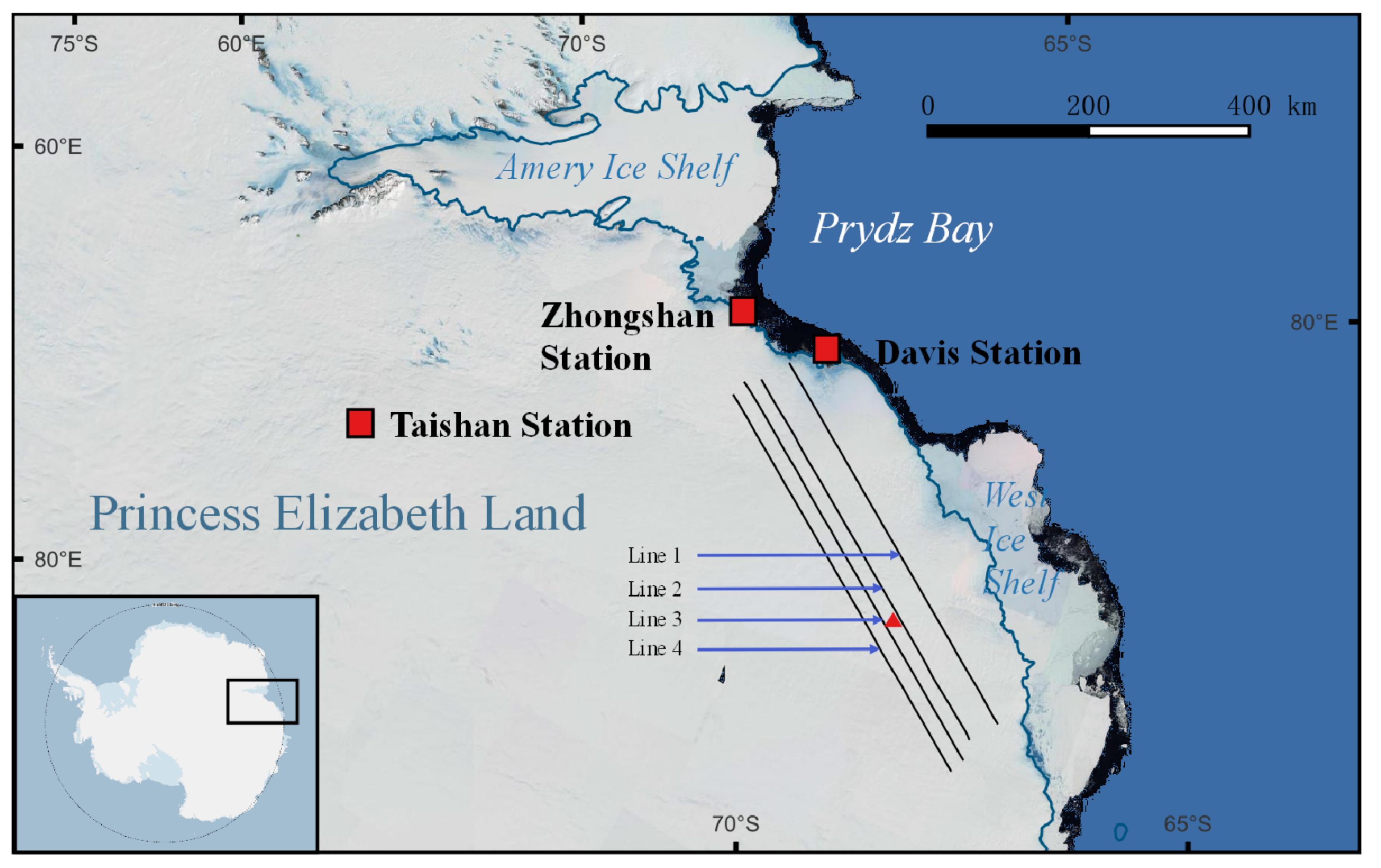
Figure 2.
(a) Ice sheet surface elevation map. (b) Ice thickness map. (c) Subglacial bedrock elevation map. (d) Magnetic data map. (e) Free air gravity data map. (f) Bouguer gravity data map. The black solid lines indicate survey lines.
Figure 2.
(a) Ice sheet surface elevation map. (b) Ice thickness map. (c) Subglacial bedrock elevation map. (d) Magnetic data map. (e) Free air gravity data map. (f) Bouguer gravity data map. The black solid lines indicate survey lines.
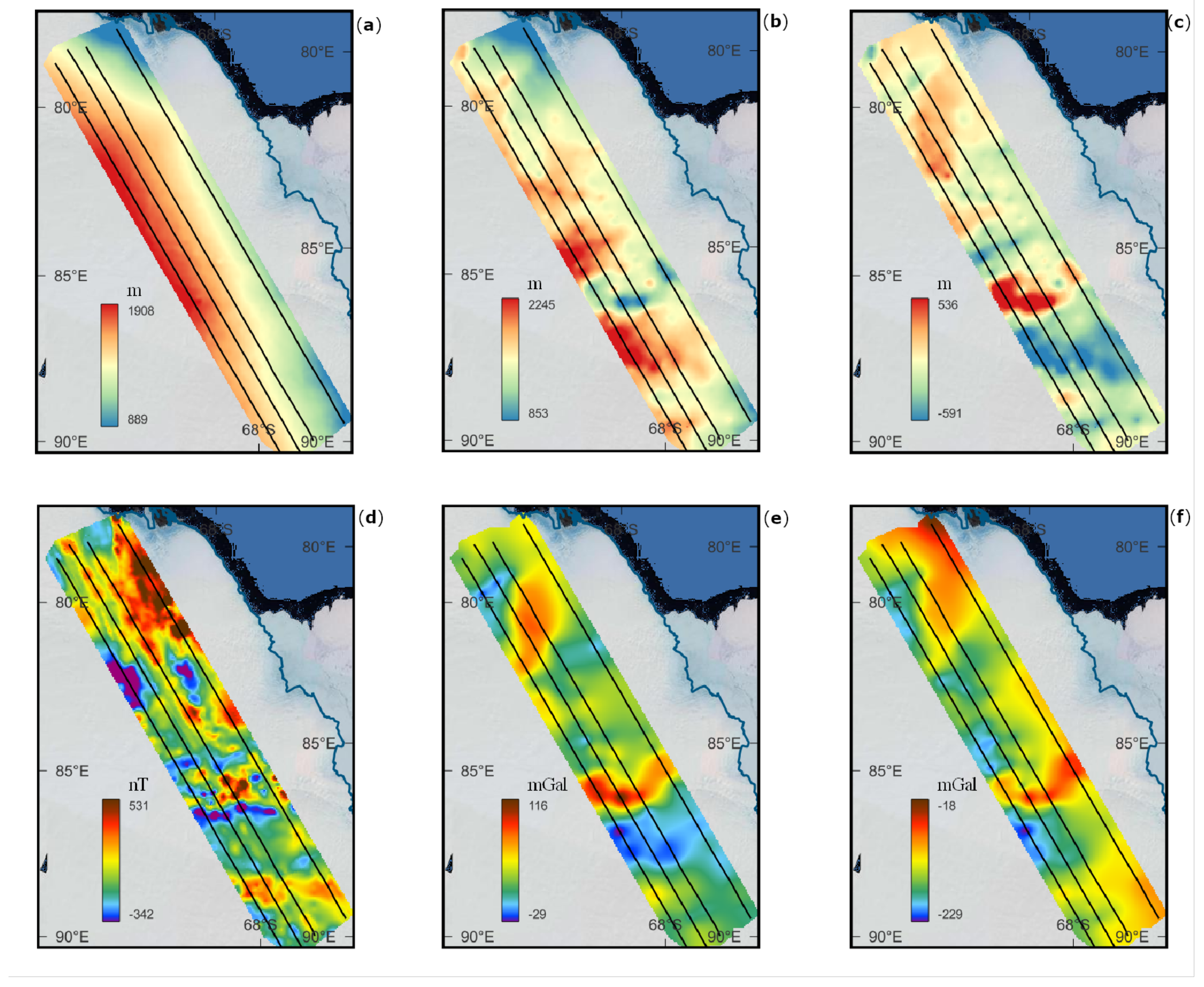
Figure 3.
Datasets and reconstructed models from survey line 1. (a) Bouguer gravity data, where black and red dots represent observed and predicted data, respectively. (b) The reconstructed density contrast model from Bouguer gravity data. Note that the density contrast value was calculated by subtracting the background density (i.e., 2.67 g/cm) from the absolute density, so the negative density contrast value represents materials whose densities are lower than the background. (c) The observed (black) and predicted (red) magnetic data. (d) The reconstructed susceptibility model.
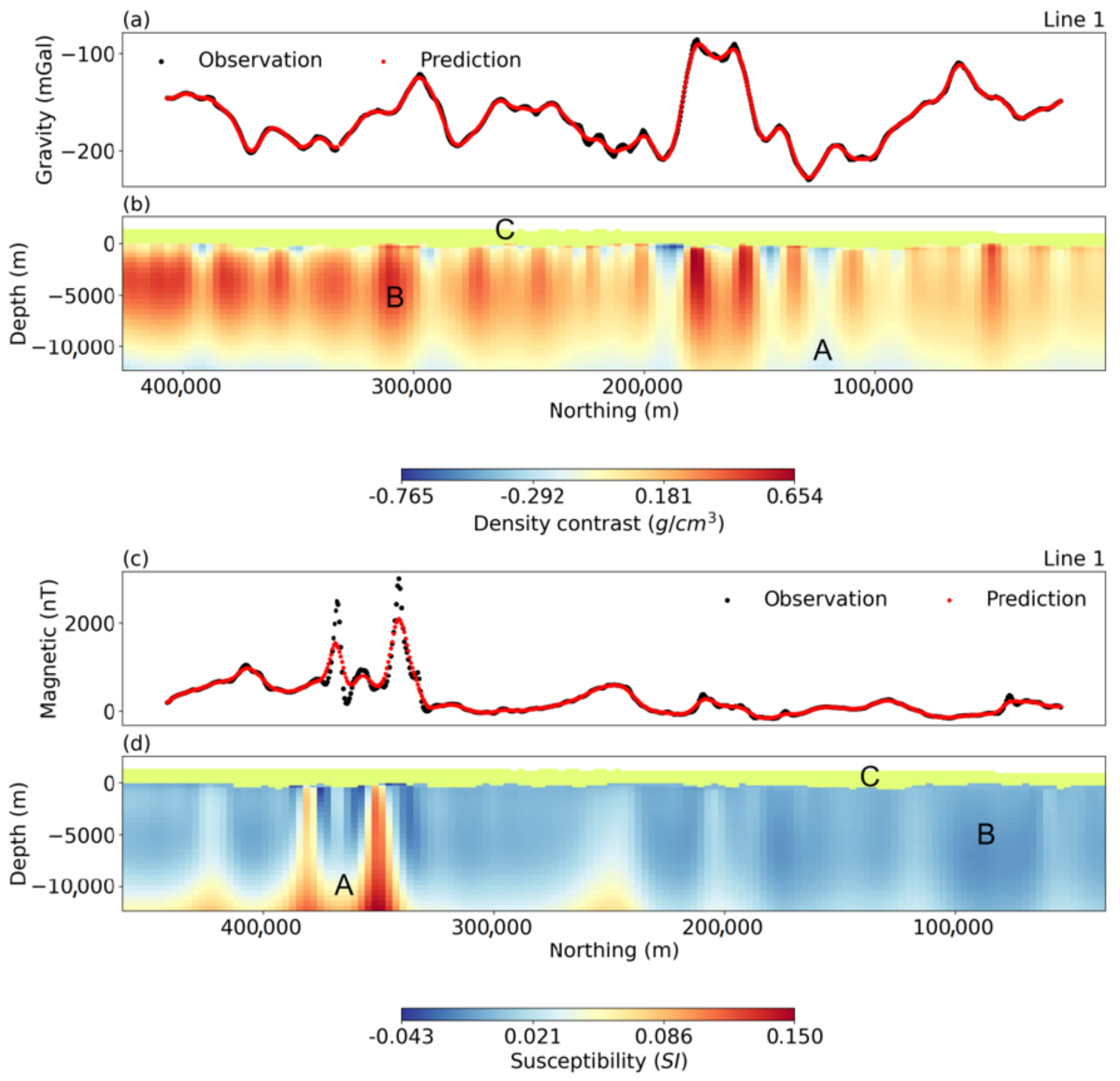
Figure 4.
Datasets and reconstructed models from survey line 2. (a) Bouguer gravity data, where black and red dots represent observed and predicted data, respectively. (b) The reconstructed density contrast model from Bouguer gravity data. (c) The observed (black) and predicted (red) magnetic data. (d) The reconstructed susceptibility model.
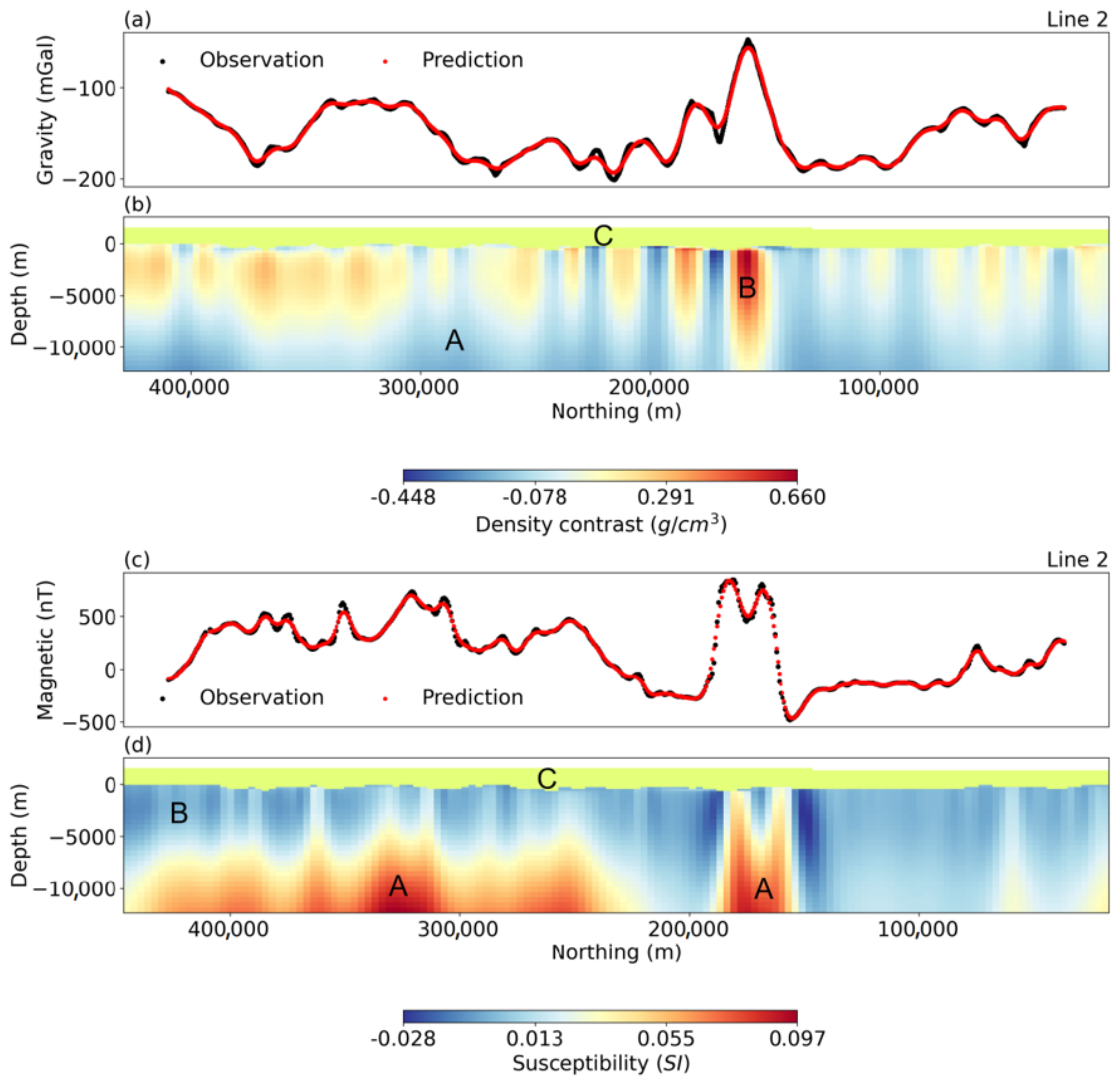
Figure 5.
Datasets and reconstructed models from survey line 3. (a) Bouguer gravity data, where black and red dots represent observed and predicted data, respectively. (b) The reconstructed density contrast model from Bouguer gravity data. (c) The observed (black) and predicted (red) magnetic data. (d) The reconstructed susceptibility model.
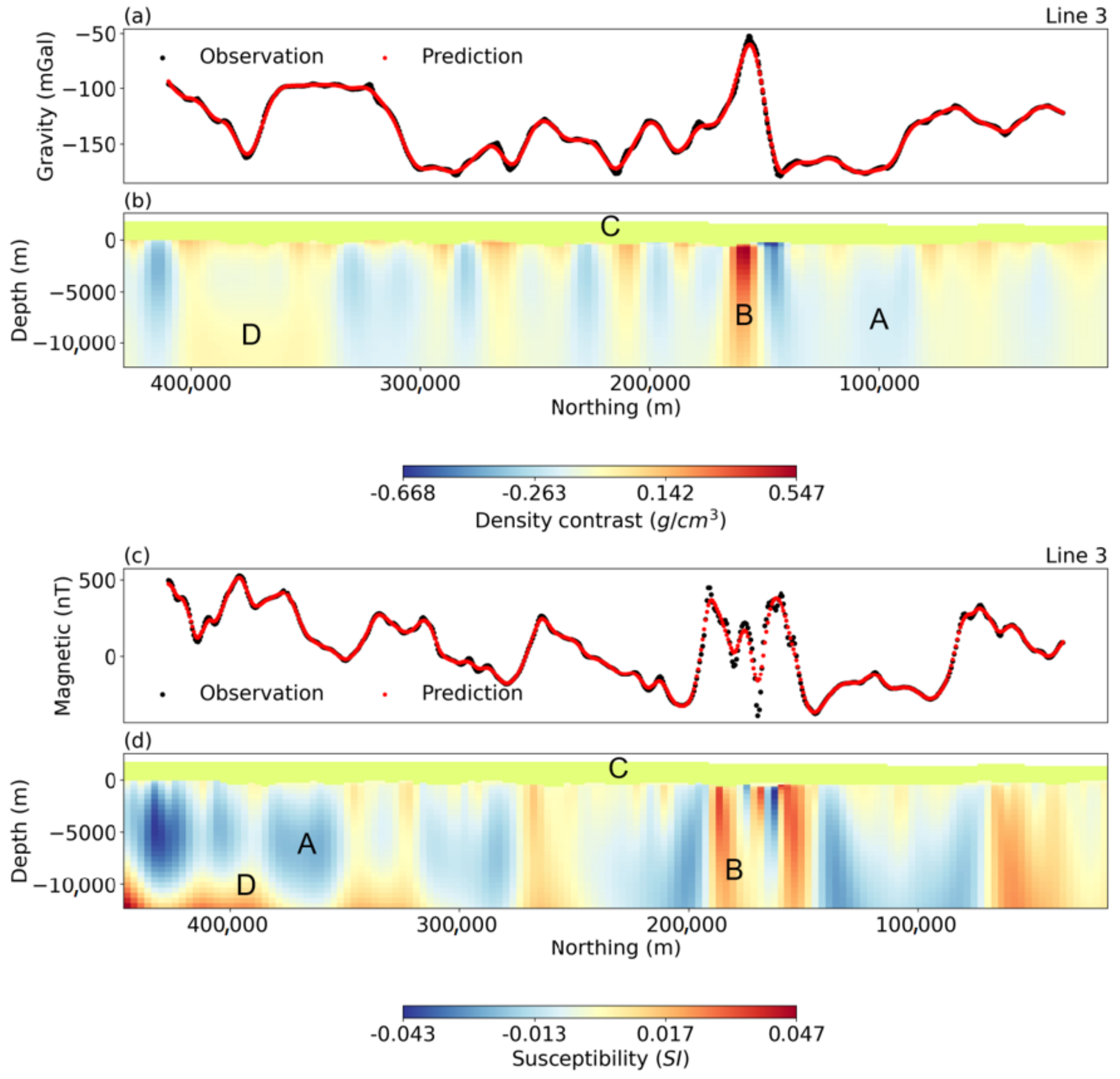
Figure 6.
Datasets and reconstructed models from survey line 4. (a) Bouguer gravity data, where black and red dots represent observed and predicted data, respectively. (b) The reconstructed density contrast model from Bouguer gravity data. (c) The observed (black) and predicted (red) magnetic data. (d) The reconstructed susceptibility model.
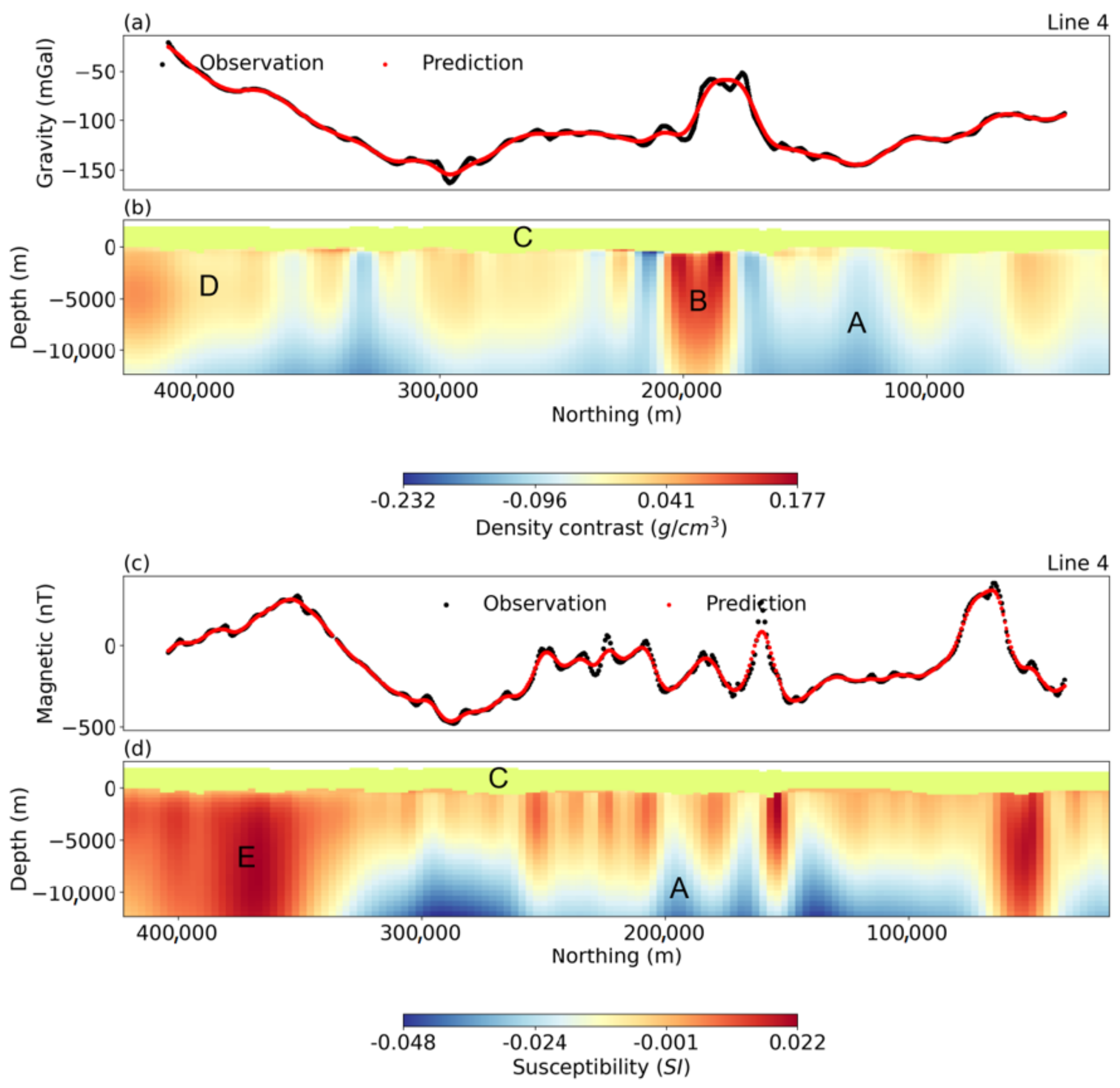
Figure 7.
(a,b) Showing the positions of the recovered susceptibility models from different viewing angles. (c) ADMAP2 magnetic data. (d) Data from the 12 aeromagnetic survey lines, where the 4 black lines are the survey lines in Figure 1 and the 8 red lines represent the new aeromagnetic data survey lines. The solid magenta lines indicate fault locations adjacent to the north–south trend.
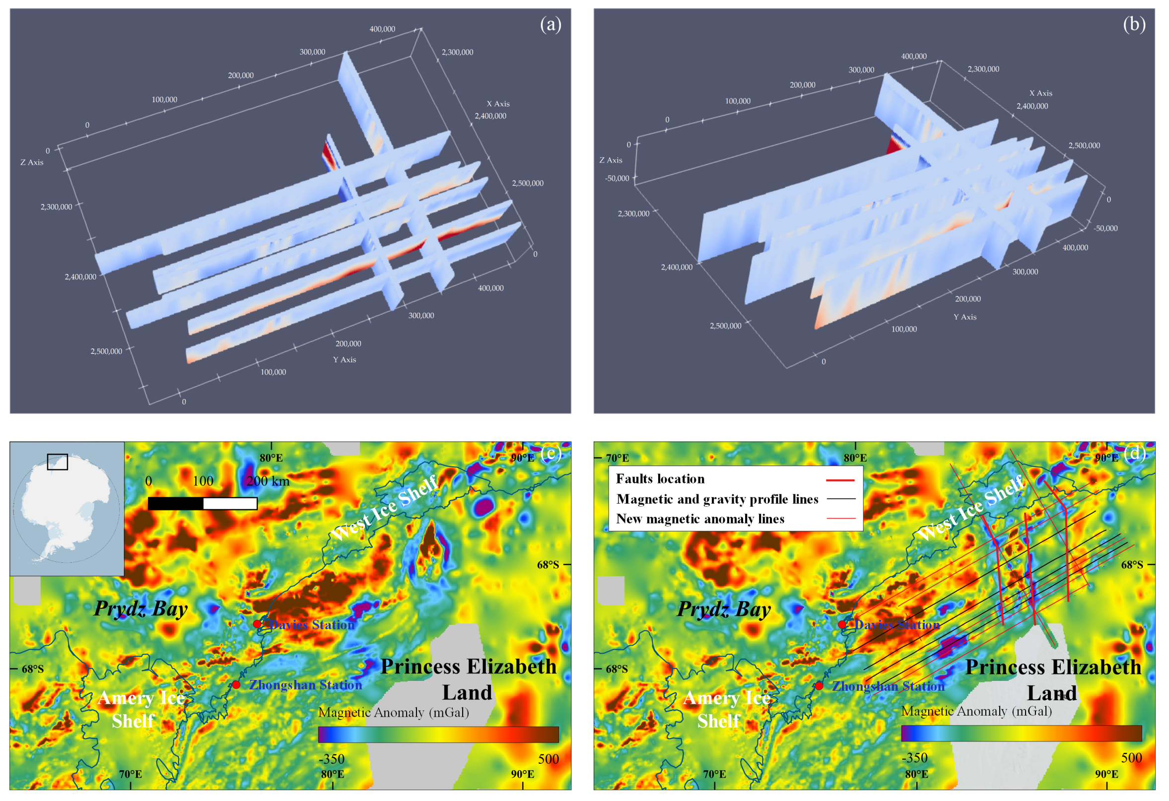
Figure 8.
(a) Map of the subglacial bedrock elevation in the Princess Elizabeth Land area of East Antarctica, generated through the analysis of ICECAP radar line data and Bedmap 2 data interpolation. The black lines are the survey lines. The red lines are the inferred faults. The 2D inversion of airborne gravity and magnetic data allowed the evaluation of different lithological distributions in the study area, as well as the identification of possible tectonic ages and faults. (b) The abundance of dominant lithological types in each profile was calculated by extracting and calculating the irregular area based on the rock physical properties of each profile. The vertical axis represents the calculated value. (c) An illustration of the rift system in some areas of East Antarctica is included, adapted from a corrected version of [2].

Disclaimer/Publisher’s Note: The statements, opinions and data contained in all publications are solely those of the individual author(s) and contributor(s) and not of MDPI and/or the editor(s). MDPI and/or the editor(s) disclaim responsibility for any injury to people or property resulting from any ideas, methods, instructions or products referred to in the content. |
© 2023 by the authors. Licensee MDPI, Basel, Switzerland. This article is an open access article distributed under the terms and conditions of the Creative Commons Attribution (CC BY) license (https://creativecommons.org/licenses/by/4.0/).
Share and Cite
MDPI and ACS Style
Li, L.; Xiao, E.; Wei, X.; Qiu, N.; Latif, K.; Guo, J.; Sun, B. Crustal Imaging across the Princess Elizabeth Land, East Antarctica from 2D Gravity and Magnetic Inversions. Remote Sens. 2023, 15, 5523. https://doi.org/10.3390/rs15235523
AMA Style
Li L, Xiao E, Wei X, Qiu N, Latif K, Guo J, Sun B. Crustal Imaging across the Princess Elizabeth Land, East Antarctica from 2D Gravity and Magnetic Inversions. Remote Sensing. 2023; 15(23):5523. https://doi.org/10.3390/rs15235523
Chicago/Turabian StyleLi, Lin, Enzhao Xiao, Xiaolong Wei, Ning Qiu, Khalid Latif, Jingxue Guo, and Bo Sun. 2023. "Crustal Imaging across the Princess Elizabeth Land, East Antarctica from 2D Gravity and Magnetic Inversions" Remote Sensing 15, no. 23: 5523. https://doi.org/10.3390/rs15235523
Note that from the first issue of 2016, this journal uses article numbers instead of page numbers. See further details here.