

A Learning Strategy for Amazon Deforestation Estimations Using Multi-Modal Satellite Imagery

Korea Aerospace Research Institute, Daejeon 34133, Republic of Korea
*
Author to whom correspondence should be addressed.
†
These authors contributed equally to this work.
Remote Sens. 2023, 15(21), 5167; https://doi.org/10.3390/rs15215167
Submission received: 7 August 2023
/
Revised: 23 October 2023
/
Accepted: 27 October 2023
/
Published: 29 October 2023
(This article belongs to the Special Issue Deforestation Detection with Deep Learning from Multispectral and Hyperspectral Satellite Images)
Abstract
:Estimations of deforestation are crucial as increased levels of deforestation induce serious environmental problems. However, it is challenging to perform investigations over extensive areas, such as the Amazon rainforest, due to the vast size of the region and the difficulty of direct human access. Satellite imagery can be used as an effective solution to this problem; combining optical images with synthetic aperture radar (SAR) images enables deforestation monitoring over large areas irrespective of weather conditions. In this study, we propose a learning strategy for multi-modal deforestation estimations on this basis. Images from three different satellites, Sentinel-1, Sentinel-2, and Landsat 8, were utilized to this end. The proposed algorithm overcomes visibility limitations due to a long rainy season of the Amazon by creating a multi-modal dataset using supplementary SAR images, achieving high estimation accuracy. The dataset is composed of satellite data taken on a daily basis with relatively less monthly generated, ground truth masking data, which is called the many-to-one-mask condition. The Normalized Difference Vegetation Index and Normalized Difference Soil Index bands are selected to comprise the datasets. This yields better detection performance and a shorter training time than datasets consisting of RGB or all bands. Multiple deep neural networks are independently trained for each modality and an appropriate fusion method is developed to detect deforestation. The proposed method utilizes the distance similarity of the predicted deforestation rate to filter prediction results. The elements with high degrees of similarity are merged into the final result with average and denoising operations. The performances of five network variants of the U-Net family are compared, with Attention U-Net observed to exhibit the best prediction results. Finally, the proposed method is utilized to estimate the deforestation status of novel queries with high accuracy.
1. Introduction
Forests occupy more than 30% of the global terrestrial surface area and serve as habitats for numerous species of plants and animals [1]. Additionally, they play a significant role in the global ecosystem by preventing soil erosion and reducing the effects of climate change via a process known as carbon cycling, which stores large amounts of carbon in the soil and releases it back into the atmosphere [2]. In particular, the Amazon rainforest covers an area of 5.5 million km2, making it the largest tropical forest, accounting for 40% of all tropical rainforest areas on Earth [3]. However, forested regions have decreased by 11,568 km2 in 2022 according to the Legal Amazon Deforestation Satellite Monitoring Project (PRODES) and the National Institute for Space Research (INPE) [4], and this decline is considered to be one of the most serious environmental problems at the present moment. The degradation of forests induces a loss of biomass and the devastation of natural resources, eventually disrupting the ecological balance and causing far-reaching changes across the globe [5]. In particular, deforested regions in the Amazon rainforest have increased from less than 100,000 km2 to more than 730,000 km2 over the past 40 years [6] according to satellite monitoring data collected by the Brazilian National Institute for Space Research (INPE). To make matters worse, the deforestation rate is increasing yearly, having increased by more than 13% in 2022 compared to the previous year [4]. This could create landslides or collapses due to soil erosion and may cause alarming animal and plant habitat losses [7]. At this rate, the role of the Amazon rainforest as a carbon sink may end by 2035, accelerating global warming significantly [8].
Analyses of changes in time-series data, necessary for understanding deforestation trends, require continuous and extensive monitoring [9]. The INPE has been monitoring the deforestation rate of the Amazon region via the PRODES and the Real-time Deforestation Detection System (DETER) since the 1980s [5]. The DETER project is based on medium-resolution satellite images and serves as an early detection tool to minimize the damage caused by deforestation. Additionally, the PRODES project provides accurate deforested area maps and calculates the annual deforestation rate [10].
Several deforestation monitoring studies have been proposed based on remote-sensing data. For the monitoring of forest cover using optical data, the Normalized Difference Vegetation Index (NDVI) is used to maximize the contrast between the background and greenery to ascertain the characteristics of green vegetation or to estimate the amount of plant biomass present on the surface via a spectral signal analysis [1,11]. Schultz et al. [12] evaluated time-series Landsat performance outcomes through various vegetation indices, including NDVI, to identify deforestation in tropical regions. DeVries et al. [13] constructed an NDVI map based on Landsat data to identify deforestation and forest degradation in Ethiopia. Alternatively, the pixel-based Break For Additive Seasonal Trends (BFAST) method can be used to detect changes based on the prediction modeling of acquired time-series data [14] for deforestation detection. BFAST detects pixels that deviate significantly from breakpoints via a time-series data analysis and expresses the type of change using different intensity levels [15]. It can be used to detect deforestation in nearly real time and can help to identify breakpoints in long-term pattern data [14,16]. Nelson [17] studied band ratios and image differencing to detect changes in the forest canopy and confirmed that vegetation index differencing yields the best performance. Meanwhile, a number of studies on deforestation characteristics using SAR as well as optics have been conducted. Field research in the Madre de Dios region of Peru [18] revealed a marked reduction in the (L-band, HV) backscatter of SAR in portions of the forest that had undergone deforestation. In addition, deforested dry forests in Bolivia exhibited a clear reduction in cross-polarized backscattering values in both the L- and C-bands [19].
The multi-sensor data fusion strategy combining SAR and optical sensors such as Landsat has improved the accuracy of forest mapping [20,21,22]. However, there are limitations to the use of a fusion method to detect forest changes, such as discrepancies in collection dates and the misalignment of multiple forms of data [23,24].
Forest research, which has classically focused on normalized vegetation indices or individual tree classification [25], has been extended to include the integrated monitoring of large regions by incorporating deep learning technology [26,27,28,29]. This state-of-the-art technology detects deforestation with the best performance, using optical and SAR datasets [30,31,32,33]. Mazza et al. [34] conducted a study on the detection of forests with high-resolution images of 5 m using various CNN networks, with the best detection performance exhibited by U-Net [35]. Using Landsat imagery, Maretto et al. [36] modified the U-Net architecture to enable the integration of both spatial and temporal contexts to detect deforestation. Torres et al. [37] evaluated the performance of different networks to detect deforestation in the Amazon rainforest based on Landsat 8 and Sentinel-2 data. Through this, it was confirmed that high-resolution Sentinel-2 images increase the detection accuracy, suggesting that high deforestation detection is possible when PRODES and deep learning technology are combined. In addition, this deep learning technology was hypothesized to detect changes in Ukrainian forests by applying Sentinel-2 data to the U-Net in Isaienkov et al. [38], and John and Zhang [39] proposed an attention U-Net [40] segmentation network to detect deforestation in the Amazon region and South America. In the Amazon and Cerrado biomes, Ortega Adarme et al. [41] evaluated patch-wise classification algorithms for the automatic detection of deforestation, finding that deep-learning-based approaches surpassed the SVM (support vector machine) [42] baseline on all performance metrics. In the context of the change detection of deforestation tasks, Soto et al. [43] proposed a domain adaptation approach that takes into account several locations in the Amazon and Brazilian Cerrado biomes to increase the accuracy of cross-domain deforestation detection. De Andrade et al. [44] extended the original DeepLabv3+ to solve class-imbalanced problems in deforestation detection in the Amazon using Landsat OLI-8 images. Zhang et al. [45] used U-Net with LSTM to detect the deforestation change in China with Sentinel-2 imagery. Islam et al. [46] analyzed forest cover changes in the Sundarbans in India with a transfer learning method using Sentinel-2A imageries from 2016 and 2022.
In general, the training strategy used for deep learning is determined by the dataset modality features. Learning based on a single modality dataset is called single-view single-network learning. On the other hand, multi-view learning strategies are applied to learn a common functional space or shared patterns with consistent high-level semantics from multi-view data obtained from multiple modalities, sources, and formats [47,48]. To provide more universal representations, the multi-view CNN architecture combines multi-view data from several sources. In this study, we propose a novel multi-view learning strategy to identify deforestation using a multi-modal dataset consisting of three different modalities.
The main contributions of this research are summarized below.
- We propose a dataset selection strategy based on a spectral index that can achieve high performance with less learning time compared to when large-capacity initial multimodal datasets are used.
- A novel multi-view learning strategy for a multi-modal satellite dataset is proposed, and it applies to diverse conditions regardless of the availability of modalities.
- The proposed fusion strategy, which combines multiple outputs from three networks, achieves high accuracy for deforestation estimations in the Amazon area.
2. Dataset
This study was planned around the region and dataset provided by the Multimodal Learning for Earth and Environment workshop (MultiEarth) [49] and consists of Sentinel-1, Sentinel-2, and Landsat 8 satellite imagery sets. The region comprises a portion of dense tropical Amazon rainforest in Pará, Brazil, containing thousands of species of broad-leaved evergreen trees, and approximately 7.2 million hectares of forest have been lost in Pará over the past 20 years [50]. The region is bounded by (4.39°S, 55.20°W), (4.39°S, 54.48°W), (3.33°S, 54.48°W), and (3.33°S, 55.20°W), as depicted in Figure 1b [51,52]. The region measures approximately 9500 km2 in area and is 80 km wide and 120 km across. The satellite images and ground truth data in the dataset covers the whole study area depicted in Figure 1.
The dataset contains synthetic aperture radar (SAR) images alongside optical imagery. Some studies have reported reduced backscatter measurements in SAR images following a deforestation event. For instance, Bouvet et al. [53] discovered a brief (5–6 months) decline in C–band vertical transmit/vertical receive (VV) values corresponding to deforested regions, consistent with patterns observed in deforested tropical forests in Indonesia [19,54].
Figure 1.
(a) Deforestation map of Brazil [55], and (b) study area in the Amazon in Brazil (2021).
Figure 1.
(a) Deforestation map of Brazil [55], and (b) study area in the Amazon in Brazil (2021).

In this study, Sentinel-1 (C-band) imagery is used, which leverages the characteristics of SAR to detect deforestation, using two polarization bands (Vertical-Vertical (VV) and Vertical-Horizontal (VH)) with a 10 m resolution. Sentinel-2 consists of twelve bands ranging from visible to shortwave infrared (SWIR) with spatial resolutions of 10 m, and Landsat 8 has eleven bands with spatial resolutions of 30 m.
All collected satellite images were divided into (256 × 256) size patches, and a single patch covers an area with a latitude and longitude range of 0.02°. The raw dataset is accessible on the MultiEarth workshop [49] webpage in the form of patches with the specified latitude and longitude range. Final patches are converted so that they have a spatial resolution of 10 m according to the masking data format. There are 69,977, 68,272, and 32,642 Sentinel-1, Sentinel-2, and Landsat 8 daily patches included in the dataset, respectively, and 17,514 monthly mask patches are used, significantly fewer than the number of daily satellite image patches.
The deforestation mask patches are generated based on Planet satellite data [56] with a spatial resolution of 3.7 m on the RGB band. In this study, we refer to the ground truth image as a ‘mask patch,’ as the deforestation estimation task is a binary classification problem (deforestation or not) [57]. The mask data consist of data captured between 2016 and 2021, excluding those captured between October and April each year, which corresponds to the rainy season in the region. The masking maker establishes the following criteria to identify deforestation areas [58]: (1) Areas that underwent the intentional felling of trees by humans are deemed to be deforestation regions. (2) Forests with continuous forest canopies exceeding 1 ha are not marked. (3) The remaining unlabeled areas where rivers with areas exceeding 1 ha pass through deforested regions are marked as deforestation regions. Finally, each pixel of the raw data is converted to 0, corresponding to forested areas, or to 1, corresponding to deforested areas. Figure 2 shows examples of three types of satellite patches and their corresponding mask patches.
A special feature of the dataset in this study is that multiple patches, taken at irregular interval days from three different satellites, correspond to a single mask patch generated on a monthly basis. Three types of satellite data are collected at different time resolutions for each month and region, and the observation frequency is irregular, meaning that the collected volume from those satellites differs even for each month. Such a problem, where multiple patches for the same area are matched to one mask patch, is known as ‘many-to-one labeling’ [59]. Given that we decided to refer to the ground truth image as ‘mask’, this problem is referred to as ‘many-to-one mask’ for the duration of this paper.
The dataset is structured with dates, locations, and corresponding mask and multi-modal source patches. Let us define the set of dates (D), locations (L), deforestation mask patches (M), patches of Sentinel-1 (S1), patches of Sentinel-2 (S2), and patches of Landsat 8 (L8), as shown in Equations (1)–(6):
where nD is a set number representing a date, nL is a set number representing a location, and (lon, lat) refers to longitude and latitude, respectively. In addition, i, j, and k, respectively, represent the number of patches for Sentinel-1, Sentinel-2, and Landsat 8 included at the given location l and on date d.
Figure 3 shows an example of the May 2018 dataset. The entire set of data for the month consists of one mask patch representing the eleven patches from three different satellites.
The entire dataset is divided into the training, validation, and test sets on a regional basis, given the strong relationship between the trait and the location. Because the pattern or aspect of deforestation can change depending on the regional characteristics, the dataset was constructed to learn regional features and prevent overfitting and erroneous learning, as opposed to using of random selection.
3. Proposed Training Strategy
3.1. Optimized Data Selection
For high-performance deforestation detection for arbitrary regions during arbitrary seasons, we constructed a multi-modal dataset in this study. Deforestation changes the reflectance of vegetation in satellite images such that suitable band selection from the different satellites is crucial to detect this phenomenon efficiently. Deforestation induces a large change in the reflectance in the shortwave infrared, vegetation red edge, and red bands [60]. Thus, B4 (Red), B7 (Vegetation Red Edge), B11 (Shortwave Infrared), and B12 (Shortwave Infrared) bands are selected for Sentinel-2, and B4 (Red), B6 (Shortwave Infrared), and B7 (Shortwave Infrared) bands are selected for Landsat 8.
The NDVI is frequently used as an indicator to extract seasonal data based on the relationship between spectral reflectance and vegetation characteristics [61]. As given by Equation (7), the RED band represents the spectral absorption by the vegetation, and the near-infrared (NIR) band accounts for the majority of change in reflectance in this case. In addition, the Normalized Difference Soil Index (NDSI, Equation (8)) uses SWIR and NIR band information, and SWIR accounts for the majority of change in the reflectance values of soil areas. Thus, the NDSI could be a good indicator for distinguishing vegetated areas from soil-degraded areas [62], and study [60] developed a model that effectively detects forests even in areas with low reflectivity caused by clouds or shadows, by combining multiple satellites and indexes. Therefore, to compose the two aforementioned spectral indices, the B8 (Near Infrared) band of Sentinel-2 and the B5 (Near-Infrared) band of Landsat 8 are additionally added to configure the dataset. Finally, eleven bands in total are selected for this study based on the aforementioned indices and related works. These are described in Table 1.
3.2. Learning Strategy
As described in the previous section, images from three different satellites are utilized in this study, and because each type of satellite data has unique characteristics, each can be recognized as a single “view”. The single-view learning strategy, described in Figure 4a, refers to training and inferring each modality’s output with only one view. In this study, there are three views that must be acquired in what is referred to as a “multi-view learning” strategy. Multi-view architectures are usually divided into multi-view-one-network and one-view-one-network strategies [63], as depicted in Figure 4.
The multi-view-one-network strategy feeds various types of data into a single network, and fused results are generated through the network. Most studies that use two or more satellite datasets utilized this method [37,39]. On the other hand, another network is employed for each view in the one-view-one-network strategy and multiple inference results are then fused during the next step.
The multi-view-one-network strategy is inappropriate for this study because the numbers of training compositions and volumes in the training set vary irregularly from month to month. Therefore, we used the one-view-one-network strategy to utilize the unique characteristics of each satellite image and to ensure applicability even when there are very few specific views that can be utilized. One of the basic principles of one-view-one-network learning is the complementary usage of information contained in multi-source data. For example, missing optical information (Sentinel-2, Landsat 8) due to harsh weather conditions can be supplemented using SAR (Sentinel-1) images, and insufficient information in Landsat 8 images owing to low image quality levels can be supplemented using Sentinel-2. As depicted in Figure 4, an independent network is trained for each view, and each trainer adopts a network that yields the optimal performance. In this study, U-Net is selected as the backbone network due to its simple network structure and good performance for segmentation. Four more U-Net variants, specifically R2U-Net [64], Attention U-Net, Attention R2U-Net [40], and Nested U-Net [65], are applied and the performance capabilities of each are compared.
3.3. Fusion Strategy
This section describes how to convert the multiple outputs from the one-view-one-network into one final result. As shown in Figure 4, the proposed training strategy consists of three steps: (1) pre-processing and input into distinct views, (2) training using the individual network, and (3) multi-output fusion and post-processing. After the pre-processing step, the three datasets were entered into the three learning models to learn the features of each view. After the training step, view-specific features were integrated into the following fusion method to obtain a compact, discriminative shape feature. That is, the fusion step aims to combine the reconstruction of multi-view features by minimizing reconstruction errors and changing the set of multiple predicted results into one representative prediction (Y).
Figure 5 depicts the entire process of deriving the final deforestation detection result through the learning strategy and the fusion method with a multi-modal dataset proposed in this study.
The problems that originate from the number of inputs from each satellite differ depending on the location and date of the patch. Therefore, the number of prediction result sets (n) used in the final output also differs. Commonly used methods in the fusion layer include deriving the average value of all multiple predicted elements (Average), adopting the only the maximum value among all output elements (Maximum), and using the trimmed mean method after limiting the maximum and minimum values of elements (Trimmed Average) [63]. These are described in Table 2 and the subscript x appearing in all formulas in Table 2 means the index of the daily data set used to predict deforestation in a specific region and month, as described in Figure 3.
All of the other fusion methods are generally calculated in a pixel-wise method and finally expressed as one 2D image. In this study, we suggest the rate of deforestation (R), which represents the deforestation rate within one predicted result (P), as described in Equation (9). If all pixels are predicted to be deforestation, the value is 100%, whereas if all pixels are predicted to be forest, the value is 0%. All of the predicted 2D images () are converted into a collection of elements representing the deforestation rate ().
In addition, we proposed a method of calculating the ‘distance similarity’ between the predicted elements (R) and mean () of the elements set, as described in Equation (10).
After certain elements with the lowest degree of similarity are eliminated according to the criteria of Equation (11), the distance similarity is recalculated with the remaining elements. Afterwards, only the elements corresponding to the condition in Equation (12) remain, indicating that the degree of similarity has become stable. In this step, eliminated elements, which have a low degree of similarity, may indicate outliers. For example, inference images with particularly low or high deforestation rates compared to other elements could have heavy cloud cover, which results in erroneous prediction results that would be removed with this procedure.
Here, n is the total number of elements constituting the initial prediction result, and m is the total number of remaining elements after Equation (11) is applied. The difference between Equations (11) and (12) is that the filtering range for the degree of similarity is different. The filtering range of Equation (11) is three sigma of the deforestation rate, which can eliminate outliers in 99.7% of the data range with the assumption of normal distribution. With this equation, we can eliminate certain outlier prediction results. Afterward, Equation (12), which has one sigma range for the rate, would wipe out additional elements with low degrees of distance similarity.
Only elements with high degrees of similarity remain after applying the proposed method, and the predicted images of matching the same index as these elements, , are averaged and regenerated as a single image. Finally, an opening operation (Equation (13)) is applied to denoise the obtained image. The opening operation (∘) involves applying an erosion operation () that removes small objects effectively, and then applying a dilation operation () that strengthens the shapes in the resulting image.
In this equation, I and M denote the image and the structuring element, respectively.
4. Results
In Section 4.1, the effects of the band selection results are presented, and the results of the proposed multi-view strategy, indicating a meaningful improvement in the prediction results, are compared to those of the single-view method in the next subsection. Finally, the effectiveness of the proposed fusion method is evaluated in the last subsection. To validate the proposed method and compare the performance capabilities from a variety perspectives, two evaluation metrics—the F1-score and Intersection over Union (IoU)—are used.
4.1. Band Selection Results
As described in Section 3.1, eleven spectral bands from three satellites were selected to comprise the dataset. We conducted experiments by altering the dataset configuration to evaluate the appropriateness of the proposed band selection method. These results are shown in Figure 6 and Figure 7. Figure 6 shows an example of the prediction results of different band selection methods for Sentinel-2. Each column depicts (a) an RGB patch of Sentinel-2 data, (b) the prediction result based on the RGB band, (c) the prediction result based all bands, and (d) the prediction result based on selected bands. True positives (deforestation) and true negatives (background), which are correct prediction results, are highlighted in green and gray, respectively. An unexpected prediction result when using only RGB bands is the high rate of false negatives, where the model failed to detect actual deforestation. In addition, when utilizing all bands, the prediction result demonstrated similarly high performance. However, training with all bands required an additional 6–7% more time and computation power in the same environment (NVIDIA 2080 Ti GPU).
Figure 7 shows the detection performance (F1-score, IoU) for different band configurations in Sentinel-2 and Landsat 8. In both cases, it can be seen that the highest performance arose when learning with the proposed selected band (green).
4.2. Multi-View Learning Effect
In this section, the results of the proposed learning strategy (one-view-one-network) are compared with those of the single-view method, which utilizes only data from a single satellite. Table 3 presents the effectiveness of the multi-view learning strategy. As described in Table 3, when the proposed multi-view learning strategy is applied, the evaluation metrics are significantly improved for every network type, meaning that the proposed multi-view learning method exhibits a superior learning performance compared to the single-view results. In addition, these performance improvements, compared to the single-view result, are identical in the U-Net family test overall.
Meanwhile, as mentioned in Section 2, the total number of mask patches in the test set is 1355. Therefore, 1355 novel queries are available for testing the proposed deforestation estimation algorithm. However, only 751 queries contain all three types of satellite imagery. These queries are known as the ‘Intersection dataset’, indicating the availability of all three types of modalities. The entire test dataset, consisting of 1355 queries, is called the ‘Expanded dataset’, indicating the availability of partial sets of modalities. Table 3 summarizes the evaluation results for single-view-based predictions and the proposed multi-view strategy-based predictions for the five different networks. The best values among each criterion are highlighted in bold.
The three cases shown in Figure 8 depict single-view results using only data from a single satellite and the prediction results with multi-modal data when using the proposed training strategy. As shown, in the single-view results, if there are heavy clouds or poor detection conditions, the final performance is reduced. However, given that the proposed model was trained under all conditions, it shows a high and stable performance regardless of exceptional conditions.
4.3. Performance of the Proposed Fusion Method
Here, we evaluate the performance of the proposed fusion method. The performance of existing fusion strategies, specifically the Average, Maximum, and Trimmed average methods, were compared with the proposed Distance similarity method.
Table 4 describes the detection performance of the four fusion strategies. The Maximum method shows the lowest performance, likely because only the maximum case was utilized without judgments of any other predicted results. In addition, the Maximum method tends to predict wider possible deforestation areas. On the other hand, the Average method shows high accuracy relative to that of the proposed model, though the high standard deviation implies that the true negative rate is very high, as shown in the first case in Figure 9. In contrast, with regard to Trimmed average, it is applied with outliers eliminated, with the result being that false positives are clearly reduced. However, as shown in the second and last examples, for Trimmed average, there is a considerable variation in accuracy depending on the image. This may have occurred because some false positives were not removed, depending on the range of the prediction results. In contrast, for the proposed method, only the prediction result that is as close to the ground truth as possible remains through the distance similarity evaluation, therefore showing similar performance outcomes in all cases.
4.4. Annual Deforestation Change Analysis
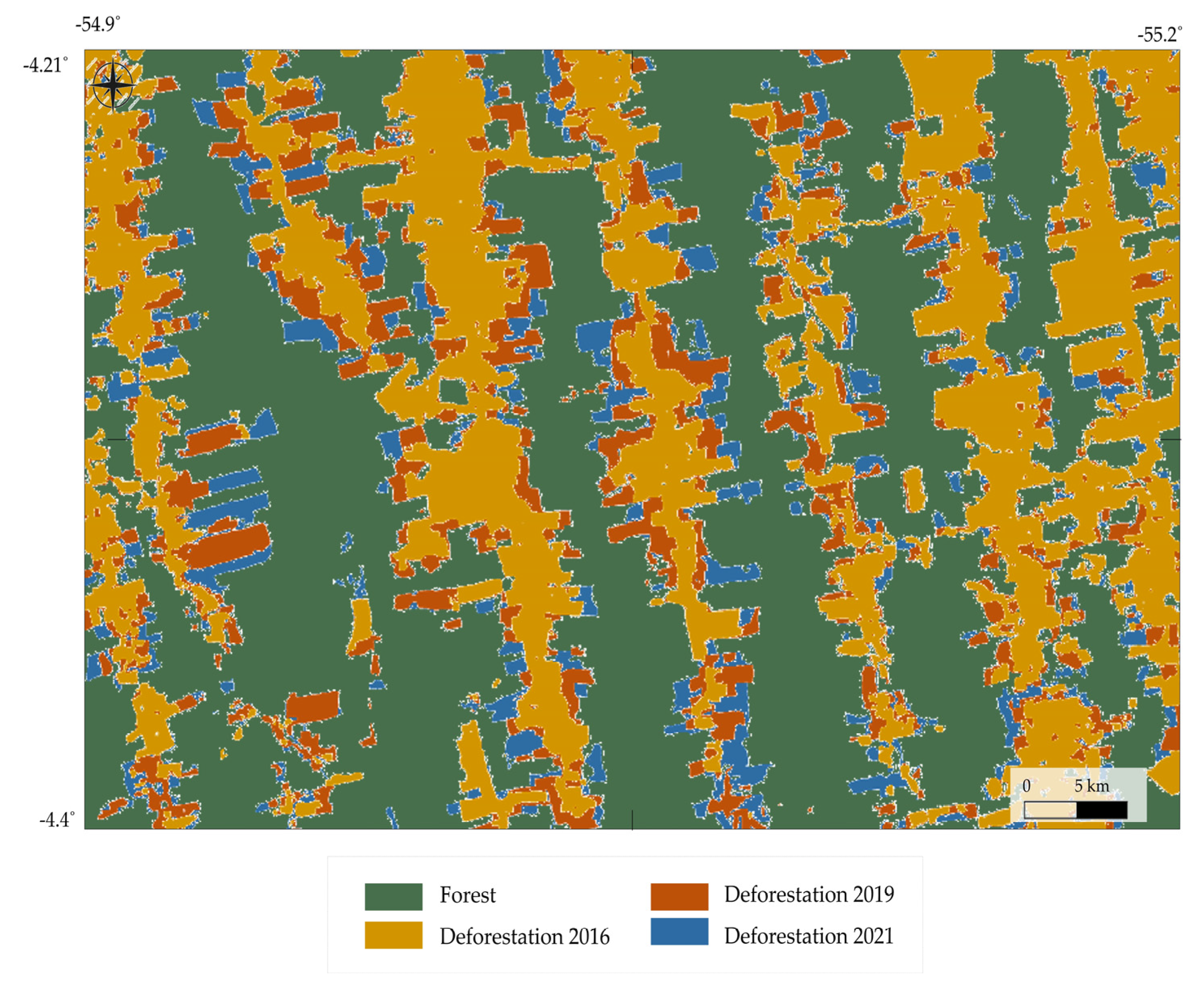
Using the proposed model, we extended the time scale to analyze the detected annual deforestation levels for the entire test area. Deforestation areas in 2016 are highlighted in yellow. The years 2016 to 2019, and 2019 to 2021, are shown in red and blue, respectively, as illustrated in Figure 10. From this color marking, it is evident that the deforested area in the test region has steadily increased over the past five years.
Similar results are observed in the annual forest loss output by Hansen et al. [66]. Hansen’s study provides various analysis results, including information on loss due to fire, as well as deforestation information for the annual global region. Since it encompasses this information, it appears to be a valuable comparative analysis tool when expanding the model to other regions in the future. Through this proposed learning strategy, this study confirmed that the model exhibits high performance and demonstrates the possibility of analyzing monthly and even annual changes, despite the limitations of daily images and monthly mask configuration.
5. Discussion
5.1. Cloudy Satellite Image Cases
In this study, a multi-modal satellite dataset containing images from three different satellites is proposed with an optimal learning strategy that can perform similarly in all environmental conditions. In this section, the model performance is discussed under various cloud conditions.
Cloudy images are classified into three types depending on the amount of cloud coverage. First, scattered clouds allow near-perfect surface visibility for humans, and, in this case, the proposed model predicted deforestation areas satisfactorily. Examples of this type and the corresponding prediction results are depicted in Figure 11 (1) under ‘Scattered Cases’. Second, more dense clouds are labeled as ‘Broken Cases’. In this case, the clouds are too thick for the surface to be observed by humans. However, the proposed method can estimate the deforestation status with high accuracy.
In the last case, the cloud cover is extremely dense, and the ground is not visible at all. These are labeled as ‘Overcast Cases’. Such cases are common in Amazonian forests, especially during the rainy season. Related research has focused on estimations of deforestation in the Amazon region [37] based on electro-optical (EO) images taken between July and August. If we trained the model with only a single optical satellite or with the single-view learning method, the model would not have detected deforested areas well. However, we can utilize multi-modal datasets, e.g., SAR images obtained from Sentinel-1 and clear images from another day, and an optimal dataset configuration with selected bands including the IR range to predict deforestation. Thus, even in the presence of overcast skies, highly accurate predictions can be obtained using other clear/SAR images.
5.2. Estimation Performance for Different Time Scales in the Many-to-One-Mask Condition
This study proposed an optimal learning strategy and fusion method for the many-to-one-mask dataset environment. The features of daily images are learned through the proposed one-view-one-learning approach, and through the fusion method it is confirmed that final high-performance monthly detection results are derived. In other words, results showing very high performances can be obtained without generating matching masks for all daily satellite images, confirming the possibility of constructing an efficient ground truth dataset. In particular, this method maintains high performance regardless of the amount of data or the composition, and it operates regardless of the satellite revisit time or in the event of data collection problems caused by weather conditions.
In addition, high detection accuracy for daily changes was confirmed by the proposed method. As shown in Figure 12, as a result of analyzing two cases with a difference of about two weeks, it was found that daily changes are clearly detected despite training based on monthly masks. Case 1 utilizes Sentinel-2 RGB patches captured on 2 July and 18 July 2017. Unlike the first result (yellow), the newly detected result (orange) identifies an expansion of approximately 6% of the deforestation area. Similarly, in case 2, it is observed that the deforestation area, which was about 11% as of 3 August 2017, increased to 17% as of 19 August 2017. This result shows that the proposed model defines deforestation areas as well as the exact ratio of the changed deforestation area.
6. Conclusions
In this study, a novel learning strategy for deforestation estimations using a multi-modal satellite dataset is presented. The dataset, which contains three different types of satellite data (Sentinel-1, Sentinel-2, and Landsat 8), consists of daily captured images and monthly masked ground truth deforestation information. The proposed multi-view learning strategy consists of three phases—optimizing data selection, multi-view learning, and result fusion. The detection performances with respect to varying input band configuration strategies—RGB, all, and selected bands, based on spectral indices (NDVI, NDSI)—are compared, and the proposed band selection was found to yield a better performance with lower computation costs. The neural networks for each satellite type are independently trained using the one-view-one-network strategy. The networks are then used to infer the individual deforestation estimation rates from each patch and the final estimation results are calculated using the proposed fusion method. It was confirmed that the optimal dataset configuration and learning strategy displayed a robust performance in all weather conditions. The prediction performances of diverse U-Net family networks (U-Net, R2U-Net, Attention U-Net, Attention R2U-Net, and Nested U-Net) were compared in terms of two evaluation metrics, revealing that Attention U-Net achieves the best predictions for both metrics. We expect that a more extensive investigation of time-series deforestation estimations could predict future deforestation risks effectively, with these results then used to formulate appropriate forest protection policies.
Author Contributions
Conceptualization, Y.C. and D.L.; methodology, Y.C. and D.L.; software, Y.C. and D.L.; validation, Y.C. and D.L.; formal Analysis, Y.C. and D.L.; investigation, Y.C. and D.L.; resources Y.C. and D.L.; data Curation, Y.C.; writing—original draft preparation, Y.C. and D.L.; writing—review and editing, Y.C. and D.L.; visualization Y.C. and D.L.; supervision, Y.C. and D.L.; project administration, Y.C. and D.L.; funding acquisition, Y.C. and D.L. All authors have read and agreed to the published version of the manuscript.
Funding
This research was supported by research on Satellite Data Applications by the Ministry of Science and ICT. This research was funded by the Korean government (MSIT) (No. 1711196030). The authors would like to acknowledge the MIT Lincoln laboratory which organized and hosted the MultiEarth 2022 workshop and provided the dataset for this research.
Data Availability Statement
All data employed in this research can be publicly downloaded at https://sites.google.com/view/rainforest-challenge/multiearth-2022 (accessed on 20 October 2023).
Conflicts of Interest
The authors declare no conflict of interest.
References
- Schroeder, T.A.; Wulder, M.A.; Healey, S.P.; Moisen, G.G. Mapping wildfire and clearcut harvest disturbances in boreal forests with Landsat time series data. Remote Sens. Environ. 2011, 115, 1421–1433. [Google Scholar] [CrossRef]
- Banskota, A.; Kayastha, N.; Falkowski, M.J.; Wulder, M.A.; Froese, R.E.; White, J.C. Forest monitoring using Landsat time series data: A review. Can. J. Remote Sens. 2014, 40, 362–384. [Google Scholar] [CrossRef]
- Hubbell, S.P.; He, F.; Condit, R.; Borda-de-Água, L.; Kellner, J.; Ter Steege, H. How many tree species are there in the Amazon and how many of them will go extinct? Proc. Natl. Acad. Sci. USA 2008, 105, 11498–11504. [Google Scholar] [CrossRef]
- Deforestation in the Amazon Remains. Available online: https://www.wwf.org.br/ (accessed on 18 October 2023).
- De Sy, V.; Herold, M.; Achard, F.; Asner, G.P.; Held, A.; Kellndorfer, J.; Verbesselt, J. Synergies of multiple remote sensing data sources for REDD+ monitoring. Curr. Opin. Environ. Sustain. 2012, 4, 696–706. [Google Scholar] [CrossRef]
- Fearnside, P.M.; Righi, C.A.; de Alencastro Graça, P.M.L.; Keizer, E.W.; Cerri, C.C.; Nogueira, E.M.; Barbosa, R.I. Biomass and greenhouse-gas emissions from land-use change in Brazil’s Amazonian “arc of deforestation”: The states of Mato Grosso and Rondônia. For. Ecol. Manag. 2009, 258, 1968–1978. [Google Scholar] [CrossRef]
- Vieira, I.C.G.; Toledo, P.D.; Silva, J.D.; Higuchi, H. Deforestation and threats to the biodiversity of Amazonia. Braz. J. Biol. 2008, 68, 949–956. [Google Scholar] [CrossRef]
- Galford, G.L.; Melillo, J.M.; Kicklighter, D.W.; Cronin, T.W.; Cerri, C.E.; Mustard, J.F.; Cerri, C.C. Greenhouse gas emissions from alternative futures of deforestation and agricultural management in the southern Amazon. Proc. Natl. Acad. Sci. USA 2010, 107, 19649–19654. [Google Scholar] [CrossRef]
- Miettinen, J.; Stibig, H.J.; Achard, F. Remote sensing of forest degradation in Southeast Asia—Aiming for a regional view through 5–30 m satellite data. Glob. Ecol. Conserv. 2014, 2, 24–36. [Google Scholar] [CrossRef]
- Diniz, C.G.; de Almeida Souza, A.A.; Santos, D.C.; Dias, M.C.; Da Luz, N.C.; De Moraes, D.R.V.; Maia, J.S.; Gomes, A.R.; Narvaes, I.S.; Valeriano, D.M.; et al. DETER-B: The new Amazon near real-time deforestation detection system. IEEE J. Sel. Top. Appl. Earth Obs. Remote Sens. 2015, 8, 3619–3628. [Google Scholar] [CrossRef]
- Eckert, S.; Hüsler, F.; Liniger, H.; Hodel, E. Trend analysis of MODIS NDVI time series for detecting land degradation and regeneration in Mongolia. J. Arid. Environ. 2015, 113, 16–28. [Google Scholar] [CrossRef]
- Schultz, M.; Clevers, J.G.; Carter, S.; Verbesselt, J.; Avitabile, V.; Quang, H.V.; Herold, M. Performance of vegetation indices from Landsat time series in deforestation monitoring. J. Appl. Earth Obs. Geoinf. 2016, 52, 318–327. [Google Scholar] [CrossRef]
- DeVries, B.; Verbesselt, J.; Kooistra, L.; Herold, M. Robust monitoring of small-scale forest disturbances in a tropical montane forest using Landsat time series. Remote Sens. Environ. 2015, 161, 107–121. [Google Scholar] [CrossRef]
- Verbesselt, J.; Hyndman, R.; Newnham, G.; Culvenor, D. Detecting trend and seasonal changes in satellite image time series. Remote Sens. Environ. 2010, 114, 106–115. [Google Scholar] [CrossRef]
- Mitchell, A.L.; Rosenqvist, A.; Mora, B. Current remote sensing approaches to monitoring forest degradation in support of countries measurement, reporting and verification (MRV) systems for REDD+. Carbon Balance Manag. 2017, 12, 9. [Google Scholar] [CrossRef]
- Hamunyela, E.; Rosca, S.; Mirt, A.; Engle, E.; Herold, M.; Gieseke, F.; Verbesselt, J. Implementation of BFAST monitor algorithm on google earth engine to support large-area and sub-annual change monitoring using earth observation data. Remote Sens. 2020, 12, 2953. [Google Scholar] [CrossRef]
- Nelson, R.F. Detecting forest canopy change due to insect activity using Landsat MSS. Photogramm. Eng. Remote Sens. 1983, 49, 1303–1314. [Google Scholar]
- Joshi, N.; Mitchard, E.T.; Woo, N.; Torres, J.; Moll-Rocek, J.; Ehammer, A.; Collins, M.; Jepsen, M.R.; Fensholt, R. Mapping dynamics of deforestation and forest degradation in tropical forests using radar satellite data. Environ. Res. Lett. 2015, 10, 034014. [Google Scholar] [CrossRef]
- Reiche, J.; Hamunyela, E.; Verbesselt, J.; Hoekman, D.; Herold, M. Improving near-real time deforestation monitoring in tropical dry forests by combining dense Sentinel-1 time series with Landsat and ALOS-2 PALSAR-2. Remote Sens. Environ. 2018, 204, 147–161. [Google Scholar] [CrossRef]
- Erasmi, S.; Twele, A. Regional land cover mapping in the humid tropics using combined optical and SAR satellite data—A case study from Central Sulawesi, Indonesia. Int. J. Remote Sens. 2009, 30, 2465–2478. [Google Scholar] [CrossRef]
- Walker, W.S.; Stickler, C.M.; Kellndorfer, J.M.; Kirsch, K.M.; Nepstad, D.C. Large-area classification and mapping of forest and land cover in the Brazilian Amazon: A comparative analysis of ALOS/PALSAR and Landsat data sources. IEEE J. Sel. Top. Appl. Earth Obs. Remote Sens. 2010, 3, 594–604. [Google Scholar] [CrossRef]
- Reiche, J.; Souza, C.M.; Hoekman, D.H.; Verbesselt, J.; Persaud, H.; Herold, M. Feature level fusion of multi-temporal ALOS PALSAR and Landsat data for mapping and monitoring of tropical deforestation and forest degradation. IEEE J. Sel. Top. Appl. Earth Obs. Remote Sens. 2013, 6, 2159–2173. [Google Scholar] [CrossRef]
- Zhang, J. Multi-source remote sensing data fusion: Status and trends. Int. J. Image Data Fusion 2010, 1, 5–24. [Google Scholar] [CrossRef]
- Lu, D.; Li, G.; Moran, E. Current situation and needs of change detection techniques. Int. J. Image Data Fusion 2014, 5, 13–38. [Google Scholar] [CrossRef]
- Achard, F.; Estreguil, C. Forest classification of Southeast Asia using NOAA AVHRR data. Remote Sens. Environ. 1995, 54, 198–208. [Google Scholar] [CrossRef]
- Lary, D.J.; Alavi, A.H.; Gandomi, A.H.; Walker, A.L. Machine learning in geosciences and remote sensing. Geosci. Front. 2016, 7, 3–10. [Google Scholar] [CrossRef]
- Khan, S.H.; He, X.; Porikli, F.; Bennamoun, M. Forest change detection in incomplete satellite images with deep neural networks. IEEE Trans. Geosci. Remote Sens. 2017, 55, 5407–5423. [Google Scholar] [CrossRef]
- De Bem, P.P.; de Carvalho Junior, O.A.; Fontes Guimarães, R.; Trancoso Gomes, R.A. Change detection of deforestation in the Brazilian Amazon using landsat data and convolutional neural networks. Remote Sens. 2020, 12, 901. [Google Scholar] [CrossRef]
- Masolele, R.N.; De Sy, V.; Herold, M.; Marcos, D.; Verbesselt, J.; Gieseke, F.; Mullissa, A.G.; Martius, C. Spatial and temporal deep learning methods for deriving land-use following deforestation: A pan-tropical case study using Landsat time series. Remote Sens. Environ. 2021, 264, 112600. [Google Scholar] [CrossRef]
- Zhao, F.; Sun, R.; Zhong, L.; Meng, R.; Huang, C.; Zeng, X.; Wang, M.; Li, Y.; Wang, Z. Monthly mapping of forest harvesting using dense time series Sentinel-1 SAR imagery and deep learning. Remote Sens. Environ. 2022, 269, 112822. [Google Scholar] [CrossRef]
- Taquary, E.C.; Fonseca, L.G.; Maretto, R.V.; Bendini, H.N.; Matosak, B.M.; Sant’Anna, S.J.; Mura, J.C. Detecting clearcut deforestation employing deep learning methods and SAR time series. In Proceedings of the 2021 IEEE International Geoscience and Remote Sensing Symposium IGARSS, Brussels, Belgium, 11–16 July 2021; pp. 4520–4523. [Google Scholar] [CrossRef]
- Irvin, J.; Sheng, H.; Ramachandran, N.; Johnson-Yu, S.; Zhou, S.; Story, K.; Rustowicz, R.; Elsworth, C.; Austin, K.; Ng, A.Y. Forestnet: Classifying drivers of deforestation in indonesia using deep learning on satellite imagery. arXiv 2020, arXiv:2011.05479. [Google Scholar] [CrossRef]
- Shumilo, L.; Lavreniuk, M.; Kussul, N.; Shevchuk, B. Automatic deforestation detection based on the deep learning in Ukraine. In Proceedings of the 2021 11th IEEE International Conference on Intelligent Data Acquisition and Advanced Computing Systems: Technology and Applications IDAACS, Cracow, Poland, 22–25 September 2021; pp. 337–342. [Google Scholar] [CrossRef]
- Mazza, A.; Sica, F.; Rizzoli, P.; Scarpa, G. TanDEM-X forest mapping using convolutional neural networks. Remote Sens. 2019, 11, 2980. [Google Scholar] [CrossRef]
- Ronneberger, O.; Fischer, P.; Brox, T. U-Net: Convolutional networks for biomedical image segmentation. In Medical Image Computing and Computer-Assisted Intervention–MICCAI 2015: 18th International Conference, Munich, Germany, Part III 18; Springer International Publishing: New York, NY, USA, 2015; pp. 234–241. [Google Scholar] [CrossRef]
- Maretto, R.V.; Fonseca, L.M.; Jacobs, N.; Körting, T.S.; Bendini, H.N.; Parente, L.L. Spatio-temporal deep learning approach to map deforestation in amazon rainforest. IEEE Geosci. Remote Sens. Lett. 2020, 18, 771–775. [Google Scholar] [CrossRef]
- Torres, D.L.; Turnes, J.N.; Soto Vega, P.J.; Feitosa, R.Q.; Silva, D.E.; Marcato Junior, J.; Almeida, C. Deforestation detection with fully convolutional networks in the Amazon Forest from Landsat-8 and Sentinel-2 images. Remote Sens. 2021, 13, 5084. [Google Scholar] [CrossRef]
- Isaienkov, K.; Yushchuk, M.; Khramtsov, V.; Seliverstov, O. Deep learning for regular change detection in Ukrainian forest ecosystem with sentinel-2. IEEE J. Sel. Top. Appl. Earth Obs. Remote Sens. 2020, 14, 364–376. [Google Scholar] [CrossRef]
- John, D.; Zhang, C. An attention-based U-Net for detecting deforestation within satellite sensor imagery. J. Appl. Earth Obs. Geoinf. 2022, 107, 102685. [Google Scholar] [CrossRef]
- Oktay, O.; Schlemper, J.; Folgoc, L.L.; Lee, M.; Heinrich, M.; Misawa, K.; Mori, K.; McDonagh, S.; Hammerla, N.Y.; Kainz, B.; et al. Attention u-net: Learning where to look for the pancreas. arXiv 2018, arXiv:1804.03999. [Google Scholar] [CrossRef]
- Ortega Adarme, M.; Queiroz Feitosa, R.; Nigri Happ, P.; Aparecido De Almeida, C.; Rodrigues Gomes, A. Evaluation of deep learning techniques for deforestation detection in the Brazilian Amazon and cerrado biomes from remote sensing imagery. Remote Sens. 2020, 12, 910. [Google Scholar] [CrossRef]
- Hearst, M.A.; Dumais, S.T.; Osuna, E.; Platt, J.; Scholkopf, B. Support vector machines. IEEE Intell. Syst. Appl. 1998, 13, 18–28. [Google Scholar] [CrossRef]
- Soto, P.J.; Costa, G.A.; Feitosa, R.Q.; Ortega, M.X.; Bermudez, J.D.; Turnes, J.N. Domain-Adversarial Neural Networks for Deforestation Detection in Tropical Forests. IEEE Geosci. Remote Sens. Lett. 2022, 19, 1–5. [Google Scholar] [CrossRef]
- De Andrade, R.B.; Mota, G.L.A.; da Costa, G.A.O.P. Deforestation Detection in the Amazon Using DeepLabv3+ Semantic Segmentation Model Variants. Remote Sens. 2022, 14, 4694. [Google Scholar] [CrossRef]
- Zhang, J.; Wang, Z.; Bai, L.; Song, G.; Tao, J.; Chen, L. Deforestation Detection Based on U-Net and LSTM in Optical Satellite Remote Sensing Images. In Proceedings of the 2021 IEEE International Geoscience and Remote Sensing Symposium IGARSS, Brussels, Belgium, 11–16 July 2021; pp. 3753–3756. [Google Scholar] [CrossRef]
- Islam, M.D.; Di, L.; Mia, M.R.; Sithi, M.S. Deforestation Mapping of Sundarbans Using Multi-Temporal Sentinel-2 Data & Transfer Learning. In Proceedings of the 2022 10th International Conference on Agro-geoinformatics, Quebec City, QC, Canada, 11–14 July 2022; Agro-Geoinformatics. pp. 1–4. [Google Scholar] [CrossRef]
- Blum, A.; Mitchell, T. Combining labeled and unlabeled data with co-training. In Proceedings of the Eleventh Annual Conference on Computational Learning Theory, Madison, WI, USA, 24–26 July 1998; pp. 92–100. [Google Scholar] [CrossRef]
- Sun, S. A survey of multi-view machine learning. Neural Comput. Appl. 2013, 23, 2031–2038. [Google Scholar] [CrossRef]
- Cha, M.; Huang, K.W.; Schmidt, M.; Angelides, G.; Hamilton, M.; Goldberg, S.; Cabrera, A.; Isola, P.; Perron, T.; Freeman, B.; et al. MultiEarth 2022—Multimodal Learning for Earth and Environment Workshop and Challenge. arXiv 2022, arXiv:2204.07649. [Google Scholar] [CrossRef]
- Turubanova, S.; Potapov, P.V.; Tyukavina, A.; Hansen, M.C. Ongoing primary forest loss in Brazil, Democratic Republic of the Congo, and Indonesia. Environ. Res. Lett. 2018, 13, 074028. [Google Scholar] [CrossRef]
- TerraBrasilis PRODES (Deforestation). TerraBrasilis. Available online: http://terrabrasilis.dpi.inpe.br/app/map/deforestation (accessed on 2 May 2023).
- GoogleEarth. Google Earth 9.185.0.0. Available online: http://www.google.com/earth/index.html (accessed on 2 May 2023).
- Bouvet, A.; Mermoz, S.; Ballère, M.; Koleck, T.; Le Toan, T. Use of the SAR shadowing effect for deforestation detection with Sentinel-1 time series. Remote Sens. 2018, 10, 1250. [Google Scholar] [CrossRef]
- Reiche, J.; Verhoeven, R.; Verbesselt, J.; Hamunyela, E.; Wielaard, N.; Herold, M. Characterizing tropical forest cover loss using dense Sentinel-1 data and active fire alerts. Remote Sens. 2018, 10, 777. [Google Scholar] [CrossRef]
- PRODES Site. Available online: http://terrabrasilis.dpi.inpe.br/app/map/deforestation?hl=en (accessed on 21 October 2023).
- Planet Team. Planet Team. Available online: https://www.planet.com (accessed on 2 May 2023).
- Fisher, R.; Perkins, S.; Walker, A.; Wolfart, E. Hypermedia Image Processing Reference; John Wiley and Sons Ltd.: London, UK, 1996; pp. 118–130. [Google Scholar]
- Scale AI. Available online: https://www.scale.com (accessed on 2 May 2023).
- Bekos, M.A.; Niedermann, B.; Nöllenburg, M. External masking techniques: A taxonomy and survey. Comput. Graph. Forum 2019, 38, 833–860. [Google Scholar] [CrossRef]
- Candra, D.S. Deforestation detection using multitemporal satellite images. IOP Conf. Ser. Earth Environ. Sci. 2020, 500, 12037. [Google Scholar] [CrossRef]
- Richard, Y.; Poccard, I. A statistical study of NDVI sensitivity to seasonal and interannual rainfall variations in Southern Africa. Int. J. Remote Sens. 1998, 19, 2907–2920. [Google Scholar] [CrossRef]
- Wolf, A. Using WorldView-2 Vis-NIR multispectral imagery to support land mapping and feature extraction using normalized difference index ratios. In Algorithms and Technologies for Multispectral, Hyperspectral, and Ultraspectral Imagery XVIII; SPIE: Bellingham, WA, USA, 2012; pp. 188–195. [Google Scholar] [CrossRef]
- Yan, X.; Hu, S.; Mao, Y.; Ye, Y.; Yu, H. Deep multi-view learning methods: A review. Neurocomputing 2021, 448, 106–129. [Google Scholar] [CrossRef]
- Zuo, Q.; Chen, S.; Wang, Z. R2AU-Net: Attention recurrent residual convolutional neural network for multimodal medical image segmentation. Secur. Commun. Netw. 2021, 2021, 6625688. [Google Scholar] [CrossRef]
- Zhou, Z.; Rahman Siddiquee, M.M.; Tajbakhsh, N.; Liang, J. UNet++: A nested U-Net architecture for medical image segmentation. In Deep Learning in Medical Image Analysis and Multimodal Learning for Clinical Decision Support; Springer: Berlin/Heidelberg, Germany, 2018; pp. 3–11. [Google Scholar] [CrossRef]
- Hansen, M.C.; Potapov, P.V.; Moore, R.; Hancher, M.; Turubanova, S.A.; Tyukavina, A.; Thau, D.; Stehman, S.V.; Goetz, S.J.; Loveland, T.R.; et al. High-resolution global maps of 21st-century forest cover change. Science 2013, 342, 850–853. [Google Scholar] [CrossRef]
Figure 2.
An example of mask patches and patches for the same region (dates: August 2017, July 2019, and May 2021, from left to right).
Figure 2.
An example of mask patches and patches for the same region (dates: August 2017, July 2019, and May 2021, from left to right).

Figure 3.
Example of the training dataset configuration: multiple daily patches obtained from multiple satellites and one representative mask patch for a month.
Figure 3.
Example of the training dataset configuration: multiple daily patches obtained from multiple satellites and one representative mask patch for a month.

Figure 4.
Approaches of single-view and two different multi-view learning strategies.

Figure 5.
Diagram of the entire process of the deforestation detection procedure proposed in this study.
Figure 5.
Diagram of the entire process of the deforestation detection procedure proposed in this study.

Figure 6.
Comparison of results obtained using different bands.

Figure 7.
Comparison of prediction performances from different band configurations for Sentinel-2 and Landsat 8 (RGB, all, and selected) based on Attention U-Net.
Figure 7.
Comparison of prediction performances from different band configurations for Sentinel-2 and Landsat 8 (RGB, all, and selected) based on Attention U-Net.

Figure 8.
Example of deforestation detection performances on different test sites (left) for the single-view and multi-view (right) methods.
Figure 8.
Example of deforestation detection performances on different test sites (left) for the single-view and multi-view (right) methods.

Figure 9.
Three examples for the fusion method performance comparison.

Figure 10.
An annual deforestation changes map of the test area: forest (green), deforestation level in 2016 (yellow), deforestation level in 2019 (red), and deforestation level in 2021 (blue).
Figure 10.
An annual deforestation changes map of the test area: forest (green), deforestation level in 2016 (yellow), deforestation level in 2019 (red), and deforestation level in 2021 (blue).

Figure 11.
Prediction examples depending on the amount of cloud coverage.

Figure 12.
Two cases of daily forest change detection results: (a1,a2) the first Sentinel-2 RGB patch, (b1,b2) the second Sentinel-2 RGB patch, (c1,c2) deforestation detection result (yellow) from first patch (a1,a2), respectively, and (d1,d2) represents the change from the first patch (a1,a2) to the second patch (b1,b2) (orange).


Table 1.
Final data specifications of the multi-modal dataset.
| Type | Selected Bands | Patch Size | Pixel Resolution |
|---|---|---|---|
| Sentinel-1 | VV, VH | 2 × 256 × 256 | 10 m |
| Sentinel-2 | B4, B7, B8, B11, B12 | 5 × 256 × 256 | 10 m |
| Landsat 8 | B4, B5, B6, B7 | 4 × 256 × 256 | 10 m (resized with bicubic interpolation from 30 m resolution) |
Table 2.
Different types of fusion strategies.
| Fusion Types | Mathematical Expression |
|---|---|
| Average | |
| Maximum | |
| Trimmed Average | |
| Distance Similarity | , |
Table 3.
Deforestation estimation performance outcomes of different networks with different dataset configurations.
Table 3.
Deforestation estimation performance outcomes of different networks with different dataset configurations.
| Network | Metric | Single-View Learning | Multi-View Learning | |||
|---|---|---|---|---|---|---|
| Sentinel-1 | Sentinel-2 | Landsat 8 | Intersection Dataset (751 Queries) | Expanded Dataset (1355 Queries) | ||
| U-Net | F1-score IoU | 0.808 | 0.711 | 0.758 | 0.889 | 0.871 |
| 0.703 | 0.634 | 0.671 | 0.812 | 0.785 | ||
| R2U-Net | F1-score IoU | 0.703 | 0.538 | 0.630 | 0.752 | 0.758 |
| 0.568 | 0.402 | 0.540 | 0.631 | 0.642 | ||
| Attention U-Net | F1-score IoU | 0.841 | 0.719 | 0.773 | 0.897 | 0.883 |
| 0.743 | 0.642 | 0.690 | 0.823 | 0.801 | ||
| Attention R2U-Net | F1-score IoU | 0.704 | 0.582 | 0.729 | 0.786 | 0.789 |
| 0.576 | 0.450 | 0.6180 | 0.677 | 0.680 | ||
| Nested U-Net | F1-score IoU | 0.811 | 0.708 | 0.760 | 0.890 | 0.874 |
| 0.705 | 0.629 | 0.673 | 0.814 | 0.789 | ||
Table 4.
Comparison of the detection performance capabilities of the different fusion methods.
| Fusion Type Metric | Average | Max | Trimmed Mean | Proposed Fusion Method |
|---|---|---|---|---|
| F1-score IoU | 0.89 (σ = 0.12) | 0.84 (σ = 0.10) | 0.87 (σ = 0.10) | 0.90 (σ = 0.10) |
| 0.81 (σ = 0.14) | 0.74 (σ = 0.14) | 0.78 (σ = 0.13) | 0.82 (σ = 0.13) |
Disclaimer/Publisher’s Note: The statements, opinions and data contained in all publications are solely those of the individual author(s) and contributor(s) and not of MDPI and/or the editor(s). MDPI and/or the editor(s) disclaim responsibility for any injury to people or property resulting from any ideas, methods, instructions or products referred to in the content. |
© 2023 by the authors. Licensee MDPI, Basel, Switzerland. This article is an open access article distributed under the terms and conditions of the Creative Commons Attribution (CC BY) license (https://creativecommons.org/licenses/by/4.0/).
Share and Cite
MDPI and ACS Style
Lee, D.; Choi, Y. A Learning Strategy for Amazon Deforestation Estimations Using Multi-Modal Satellite Imagery. Remote Sens. 2023, 15, 5167. https://doi.org/10.3390/rs15215167
AMA Style
Lee D, Choi Y. A Learning Strategy for Amazon Deforestation Estimations Using Multi-Modal Satellite Imagery. Remote Sensing. 2023; 15(21):5167. https://doi.org/10.3390/rs15215167
Chicago/Turabian StyleLee, Dongoo, and Yeonju Choi. 2023. "A Learning Strategy for Amazon Deforestation Estimations Using Multi-Modal Satellite Imagery" Remote Sensing 15, no. 21: 5167. https://doi.org/10.3390/rs15215167
Note that from the first issue of 2016, this journal uses article numbers instead of page numbers. See further details here.