

A Grid-Based Gradient Descent Extended Target Clustering Method and Ship Target Inverse Synthetic Aperture Radar Imaging for UHF Radar

1
The School of Electronic Information, Wuhan University, Wuhan 430072, China
2
The Wuhan Shipboard Communication Institute, Wuhan 430072, China
*
Author to whom correspondence should be addressed.
Remote Sens. 2023, 15(23), 5466; https://doi.org/10.3390/rs15235466
Submission received: 25 August 2023
/
Revised: 17 November 2023
/
Accepted: 21 November 2023
/
Published: 23 November 2023
(This article belongs to the Special Issue Application of Shore-Based, Sky-Based and Marine Radars to Ocean and Target Parameter Extraction)
Abstract
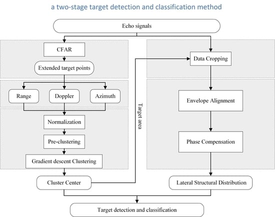
:Inland shipping is of great significance in economic development, and ship surveillance and classification are of great importance for ship management and dispatch. For river ship detection, ultrahigh-frequency (UHF) radar is an effective equipment owing to its wide coverage and easy deployment. The extension in range, Doppler, and azimuth and target recognition are two main problems in UHF ship detection. Clustering is a necessary step to get the center of an extended target. However, it is difficult to distinguish between different target echoes when they overlap each other in range, Doppler, and azimuth and so far practical methods for extended target recognition with UHF radar have been rarely discussed. In this study, a two-stage target classification method is proposed for UHF radar ship detection. In the first stage, grid-based gradient descent (GBGD) clustering is proposed to distinguish targets with three-dimensional (3D) information. Then in the second stage, the inverse synthetic aperture radar (ISAR) imaging algorithm is employed to differentiate ships of different types. The simulation results show that the proposed method achieves a 20% higher clustering accuracy than other methods when the targets have close 3D information. The feasibility of ISAR imaging for target classification using UHF radar is also validated via simulation. Some experimental results are also given to show the effectiveness of the proposed method.
1. Introduction
Inland shipping is indispensable to trade, transportation, and tourism. With the fast growth of inland shipping, the surveillance of ships becomes a more and more important task which is of great significance for the management and dispatch of ships [1]. Meanwhile, ship target classification and identification are also of great significance in providing support for a good inland shipping environment [2]. Ultrahigh-frequency (UHF) radar is an effective equipment for ship detection [3,4] which is also capable of river hydrological monitoring [5]. These dual uses make UHF radar play a more important role in inland river monitoring than other ship surveillance means.
The other means for inland ship surveillance include automatic identification system (AIS) [6,7], video surveillance [8,9,10], wireless sensor network [11], and synthetic aperture radar (SAR) imaging [12,13,14]. Limitations are obvious in these methods. Small ships are often not subject to surveillance by AIS since only those big enough ships are demanded to be equipped with AIS. Video surveillance is susceptible to weather conditions such as rain and snow. Wireless sensor network often has a high cost since it demands lots of sensors and the detection range is short. SAR system can provide a high resolution but it is difficult to perform real-time monitoring and the cost is much higher. In contrast, UHF radar is more suitable for inland ship detection due to its low cost of setup and maintenance and long detection range (up to >1 km) [15].
In UHF radar inland ship detection, one main problem is that the range and azimuthal resolution are much smaller than the ship size (e.g., 100 m). The ship echoes will occupy more than one resolution cell and form an extended target (or point cloud) on the range-Doppler spectrum (RDS) [16] as well as the angular spectrum. To handle such extended targets, specific target points should be detected first. The range and Doppler of target points can be obtained from the RDS by constant false alarm rate (CFAR) methods which are commonly used for ship detection [3,17]. For small-aperture UHF radar as used in this study, direction finding [18,19] is then performed for each target point to determine the specific positions of the ship, which also leads to extension in the azimuthal domain. Consequently, clustering is necessary to get the accurate position of a ship, and then the cluster centers are used to obtain the necessary state parameters of the ship. By monitoring the motion parameters of each target, the positions of the targets can be obtained. Moreover, in order to facilitate more efficient tracking and management of various vessels, we aim at detecting and recognizing the targets.
In recent years, ship detection with deep learning (DL) methods has attracted great attention due to their promising performance in classification accuracy [20,21,22]. However, DL methods require substantial labeled data for training. Because the dataset is quite few, ship detection with UHF radar is hard to implement with DL methods. Therefore, the classical modeling method is a practical choice.
There are already some methods for clustering extended target points, but some may not be directly used for ship detection with UHF radar. Chi et al. proposed a new extended target tracking method based on clustering by fast search and find of density peaks (CFSFDP) algorithm [23]. It relies on a centralized density distribution of the extended target points (high-density points surrounded by low-density ones), but the density in radar RDS in this study is nearly uniformly distributed. Li et al. partitioned the extended target measurement set with a clustering algorithm based on kernel fuzzy C-means (KFCM) [24], but it requires a preset number of clusters which is impossible in ship detection. So far, the clustering methods suitable for UHF radar mainly include two-dimensional (2D) and three-dimensional (3D) approaches. One popular 2D clustering method suitable for target points with uniform density is the density-based spatial clustering of applications with noise (DBSCAN) [25]. Kuang et al. also proposed another 2D clustering method for extended target clustering with UHF radar [26]. One problem in the 2D clustering methods is that, it may be incapable of distinguishing between different targets when they are close in a 2D (e.g., range and Doppler) space. Therefore, clustering methods based on 3D (e.g., range, Doppler, and azimuth) information have also been proposed to obtain the clustering center for extended target [27,28]. Thresholds are used for clustering in three dimensions, but [27] groups the extended target points sequentially whereas [28] associates the points on neighboring grids with iteration. However, they still cannot distinguish the targets efficiently when the range, Doppler, and azimuth of different ships are all close.
To address this problem, a grid-based gradient descent (GBGD) clustering algorithm is proposed here to achieve the cluster center of extended ship targets detected by UHF radar. Firstly, the 3D space of range, Doppler, and azimuth are divided into grids and a normalization is performed. Then, grid resolutions are adjusted to pre-cluster and remove some obvious interference points. Finally, the clusters are grouped according to the relationship between the target motion state and the steepest gradient descent on the grid. This is why the proposed GBGD clustering algorithm can distinguish targets with similar 3D information, whereas the traditional 2D and 3D clustering methods cannot. And, it allows the detection to be adapted to more scenarios. Since it is extremely difficult for the radar to distinguish between targets with the same location and speed, the situation discussed here is generally limited to targets with similar ranges and Doppler but different azimuths.
After the clustering, the positions of the targets can be obtained. To further determine the target types, it is essential to perform target classification. So far, research and discussions on the identification and classification of ship targets with UHF radar have been quite few. Target classification approaches have been tried based on optical images [29,30,31,32,33] and SAR and inverse synthetic aperture radar (ISAR) images [32,33,34]. Wherein, Karine et al. recognized radar targets using salient keypoint descriptors and multitask sparse representation based on X-band SAR or ISAR images [32]. Ni et al. achieved high-precision classification for ISAR images using contrastive learning [33]. Musman et al. presented a capability for automatic recognition of ISAR ship imagery [34]. It is evident that ISAR imagery has become an effective means for target classification. Therefore, we try to apply the ISAR imaging approach to differentiate different target types with UHF radar.
Consider the scenario of inland ship detection, the long integrated time, low target velocity, and simple motion model are beneficial to ISAR imaging since they can offer a high cross-range resolution in theory. However, there are still some challenges which need to be addressed. UHF radar has a relatively lower resolution compared with high-resolution radar, especially in range resolution, which makes it difficult to differentiate target types in the range domain. Moreover, in the context of inland ship target detection, there is significant interference from river clutter and shoreline clutter. To perform better ISAR imaging, it is necessary to eliminate clutter interference based on the target’s position. Due to the temporal stability of shore clutter and river clutter, they typically exhibit minimal variations over a radar dwell. This similarity can lead to a situation in ISAR imaging where the overall similarity is high, but the envelopes of certain parts of the target cannot be properly aligned. Therefore, it is necessary to perform extended target point detection and clustering to obtain the target’s extent before proceeding with the ISAR imaging process. In this study, the ISAR imaging method is applied, which allows for achieving a relatively high cross-range resolution, enabling the extraction of the lateral structural distribution of the target at a specific angle, which serves as the basis for distinguishing different types of targets.
The remainder of this paper is organized as follows. Section 2 describes the characteristics of the UHF ship detection and the ISAR signal model. The specific proposed methods are presented in Section 3. Results of simulations and real data are given in Section 4. Section 5 gives some discussions. Section 6 gives a brief conclusion.
2. Characteristics of Extended Ship Target and ISAR Signal Model
2.1. Characteristics of Extended Ship Target
The schematic diagram of inland ship detection with a UHF radar is shown in Figure 1. Assume that the antenna baseline is parallel to the riverbank and in each radar dwell ship sails in the river with uniform linear motion. Let R be the distance between the ship and the radar, the azimuth of the ship with respect to the perpendicular of the riverbank, v the speed, and the radial velocity. The relationship between v and is given by:
The UHF radar is able to position the ship by the estimates of R, , and . and R can be read from the RDS as shown in Figure 2. In this study, the UHF radar works at 340 MHz with a chirp bandwidth of 10 MHz. The corresponding resolutions of the range and radial velocity are 15 m and 0.086 m/s, respectively. Since the resolution is often much finer than the ship length, extension occurs in range, Doppler, and azimuth.
As can be seen from Figure 2, due to the relatively high resolution of UHF radar, the ship echo occupies more than one cell in the RDS. When there are more than one ship with similar ranges and Dopplers, it is difficult to distinguish them from the RDS. However, a 3D clustering method is able to handle this if the azimuths are significantly different. When two or more ships have similar radial velocities, ranges, and azimuths, the existing 3D clustering methods can no longer distinguish between them. In this study, we consider using the motion state as a basis to distinguish between different ships. The azimuth is and changes monotonically. The radial velocity depends on both the magnitude and direction of the speed. According to the sign of radial velocity, the state of motion can be divided into approaching and leaving the radar. Therefore, it is possible to distinguish between different targets that cannot be distinguished by the 3D clustering methods in the RDS with their motion features.
2.2. Characteristics of ISAR Signal Model
To perform ISAR imaging, the UHF radar ship detection scenario can be simplified as the target moving in a straight line at a uniform velocity on a 2D plane like Figure 3a. where is the angle between the radar line of sight and ship moving direction at the beginning, is the angle of rotation during the whole observation time. The target moves from left to right along the horizontal dashed line in Figure 3a (from a to b). The movement of the target can be divided into two parts, i.e., radial motion (from a to c) and angular rotation (from c to b). The part of the radial motion is useless for ISAR imaging, it should be compensated. Figure 3b shows the process of a specific scatter point in the target rotating between adjacent echoes. Where O is the center of rotation of the target, the x and y axes represent the cross-range and range dimensions respectively. The direction of the radar wave is the same as the y-axis. In this scenario, the radar waves are plane waves and propagating from below, as indicated by the row of arrows below the x-axis in Figure 3b. p is the scattering point before rotating while p’ is after rotating. and are the coordinates of the scattering point p relative to O. is the distance between p and O. is the angle between p and x axis, is the angle of rotation. During such a rotation, the radial displacement of the scattering point can be written as:
The formula of a derivative is
where the here is , and the is close to 0 between adjacent echoes. Equation (3) is rewritten as:
The phase difference of the adjacent echoes caused by radial displacement is
Equation (11) illustrates the phase difference between two adjacent echoes is proportional to the . There is a phase rotation factor that differs between two adjacent echoes. As the scattering point undergoes continuous rotation, the resulting change in the echo’s phase is manifested as Doppler. Assuming that the scattering point continues to rotate till receiving N echoes, the phase difference is:
where is the cross-range difference between the scattering point before rotating and after rotating. When , it is considered that two different targets can be distinguished, so the cross-range resolution is:
where is the angle of rotation during the whole observation. The range resolution is:
When the is too large, migration through the resolution cell of scattering points will affect the image quality. Hence, it is typically necessary for the target size and resolution to fulfill the following criteria:
In the UHF radar inland ship detection scenario, the condition of Equation (15) is satisfied. The specific parameters are shown in Section 4: is 0.88 m, and are 100 m and 20 m, and are 5.13 m and 15 m, respectively. By substituting these parameters into the equation and performing the calculation, it can be confirmed that Equation (15) holds true.
3. Proposed Methods
3.1. Clustering Algorithm
In this study, the clustering algorithm is performed after the candidate extended target points in the RDS are obtained by a CFAR detector. As shown in Figure 4, there are three main steps in clustering, i.e., normalization, pre-clustering, and gradient descent clustering.
3.1.1. Normalization
The proposed clustering algorithm needs information in three dimensions, which should be normalized first. The RDS has divided the extended target points into a 2D grid with a range cell of and a Doppler cell of . Azimuth is then added with an azimuthal cell of to form a 3D grid. The set of the extended target points, T, in the 3D grid can be denoted as:
where M and N are the numbers of cells in Doppler and range, K is the total number of extended target points, , , and are the range, radial velocity, and azimuth of the i-th target point , and , , and are the normalized coordinates, respectively. represents the ceiling operator.
3.1.2. Pre-Clustering
- Divide the grid into several big chunks. The chunk sizes here are chosen as 8 cells for range and Doppler and 20 cells for azimuth.
- Calculate the attribute parameters of each chunk, including the mean and variance of the range, Doppler, and azimuth.
- Remove discrete false points based on azimuth concentration and the number of points in each chunk. The extended target points are numerous, and their azimuth distribution is concentrated, while the false points perform the opposite characteristics. These properties can be used as a basis to eliminate false points. The associated chunks are then grouped into the same cluster.
3.1.3. Gradient Descent Clustering
The azimuths of extended points in each cluster given by pre-clustering are first ordered. Then each point is tested whether it matches the conditions for association with the existing clusters. The association conditions include range, Doppler, azimuth, and gradient descent direction. For each 2D grid point , there exists a scalar . The gradient of Doppler on the 3D grid is given by:
where is the distance in the Doppler cell between the two points. Since the target points are searched by azimuth in descending order, the gradient is also in descending order. The gradient descent direction can be considered as an associated condition. The specific process of gradient descent clustering is outlined in Algorithms 1 and 2. The entire workflow of the proposed clustering method is depicted in Figure 5, which shows the proposed clustering method is comprised of three stages: (1) normalization, (2) pre-clustering, and (3) Gradient descent Clustering.
| Algorithm 1: GBGD-Cluster |
 |
| Algorithm 2: Associate |
| Data: , , and are the thresholds for m, n, and in Equation (16), respectively. Set , , . C is an existing cluster created by GBGD-Clustering. Input: cell under processing b. the end cell of an existing cluster c  |
3.2. ISAR Imaging Method
The primary purpose of this work is to demonstrate the effectiveness of applying ISAR imaging methods to UHF radar inland ship detection and classification scenarios. As a result, we use the classical range-Doppler imaging algorithm to generate ISAR images, and the concepts of envelope alignment and phase compensation will be introduced below [35,36].
3.2.1. Envelope Alignment
During the coherent integrated time (CIT), the target is constantly moving. It may lead to signals from the same scattering point being centered at different range cells in different echoes. To align these signals from the same scattering point, it is necessary to shift the signals from different echoes to bring them together in the same range cell. This process is envelope alignment.
The envelope alignment method used here is the typical peak method [37]. Firstly, the first strong peak of the strongest pulse within the CIT is taken as the reference. Next, the peaks of other pulses are aligned to the reference peak in the range domain. This method is employed because ship targets generally have higher energy than the clutter. It should be noted that the clutter should be removed before envelope alignment to avoid failure of using the peak method in real data.
3.2.2. Phase Compensation
After envelope alignment, the phases of the echo signals are disordered, which makes imaging difficult without phase compensation. Since all range cells share the same initial phase sequence, a dominant scattering point can be selected to estimate the phase difference between different echoes for phase compensation. Moreover, multiple dominant scattering points can improve SNR and enhance the accuracy of phase compensation. So, we use the multiple dominant scattering points method to compensate phase. The specific steps of the method are illustrated below. Firstly, it is necessary to eliminate phase components that vary with the number of the echo to ensure the phase coherence of dominant scattering points. Then, phase compensation is performed by estimating the initial phase sequence with these dominant scattering points.
Assume that the rotation angle is small and the target rotates at a constant speed, the k-th range cell with only one scattering point. The echo envelope can be written as:
where and are the amplitude and phase caused by the weak clutter and noise. M is the number of all echoes. is the initial phase, is the phase when , and is the distance in cross-range axis. Let the m-th echo which shown in Equation (19) multiply the conjugate of the ()-th echo, the result is given by:
where is the difference of initial phase. is the phase difference between the adjacent echoes caused by noise and clutter. It can be seen that there is no in Equation (19) and the become which is no longer relevant to m. Moving the peak of cross-range data of each range cell to the middle of the image. It can eliminate the . Then do the conjugate multiplication. N is the number of all dominant scattering points. The Equation (20) is rewritten as:
If noise and clutter satisfy the Gaussian distribution, the value of the initial phase difference can be estimated from Equation (21) using the maximum likelihood estimation method. The result is written as:
After phase compensation, the moving target can be converted into a rotating target, which can be used for ISAR imaging.
4. Results
This section will respectively give the simulation results of the proposed clustering algorithm and the ISAR imaging in UHF first. Then the field experimental results will be shown to illuminate the effectiveness of the proposed methods.
4.1. Simulation Results
4.1.1. The GBGD-Clustering Algorithm
The detection scenario of the simulation is shown in Figure 1, and simulated radar parameters are introduced in Table 1.
In the simulations, the partition-based detection method is employed for adaptive CFAR detection. Cells average CFAR method is used in regions with weaker clutter on both sides, while the CFAR method joint time dimension is used in the region with stronger clutter in the middle of the RDS, The CFAR detectors are implemented with a nominal probability of false alarm rate Pfa = . The proposed clustering method parameters are described in Section 3, including pre-clustering with a range and Doppler of 8 cells, azimuth of 20 cells. For the subsequent gradient descent clustering, the threshold for range, Doppler, and azimuth are empirically set to 4, 2, and 7, respectively.
Four ships are simulated to evaluate the clustering algorithms, as shown in Figure 6. The signal-to-noise ratios (SNR) are all set to be 30 dB. The ships’ center motion parameters are given in Table 2. These ships can be divided into two pairs. The pair of Target 2 and Target 3 simulates the scenario that 3D coordinates are all close and the other pair is in the condition that the range and Doppler parameters are close while the azimuths are different. Intermediate frequency (IF) signals are simulated according to these parameters. Then, the IF signals are added to the actual river clutter echoes without ships. Since the real width of the river is about 500 m, there are 41 range cells selected here to match the actual situation. Figure 6a shows the detected points which are indicated by black ‘∗’ in the RDS. The real positions and azimuths of each target in the range-Doppler matrix are shown in Figure 6b and Figure 6c respectively.
The performances of the four clustering algorithms, i.e., DBSCAN [25], 3D group sequentially (3DGS) clustering [27], grid-based (GB) clustering [28], and GBGD-clustering, which can be used for UHF radar detection, are shown in Figure 7. In each subfigure, the classes of targets are represented by colored symbols. As shown in Figure 7a, only two targets are detected, indicating that the targets with adjacent range and Doppler parameters cannot be distinguished using the 2D clustering method. Figure 7b,c shows that the targets with adjacent range and Doppler parameters can be discriminated using the azimuth information. It is noteworthy that only the proposed GBGD-clustering algorithm can distinguish all the targets, as shown in Figure 7d. The 3DGS-clustering and GB-clustering methods are not able to distinguish target 2 and target 3 since their azimuths are also close. It can be preliminarily shown that the proposed method outperforms the others.
For the three 3D methods, the clustering accuracy (Acc) and the offsets between the cluster centers and the real target centers are evaluated by 300 Monte Carlo trials under the conditions mentioned in Figure 6. The results are listed in Table 3. The Acc is a classic external validation index for clustering.
It can be seen from Table 3 that the three methods achieve similar results in terms of Acc and the target center offset. This is because Target 1 and Target 4 have significantly different azimuths, and all three 3D clustering methods can distinguish them. However, for Target 2 and Target 3, the offset obtained by the proposed method remains close to 0, while the other two methods appear significant deviations in both range and azimuth. Furthermore, the GBGD method also achieves an Acc value closest to 1. So, in general, the proposed method obtains the best performance in Acc and offset. Moreover, only the proposed GBGD clustering method can correctly differentiate targets with close azimuths, e.g., Target 2 and Target 3.
In order to further verify the stability of the proposed method, 300 Monte Carlo trials are conducted under different SNR conditions. Target 2 is selected as the observation object in the following simulations since it has the most prominent improvement.
Figure 8 shows the results of Acc. It can be seen that the clustering accuracy of the proposed GBGD clustering method increases as the SNR increases, and is remarkably higher than the Acc of the other two methods, i.e., 35% higher than the 3DGS-clustering and 20% higher than the GB-clustering. According to Figure 6c, both Target 2 and Target 3 have some extended points around 0° in azimuth. At a high SNR level, the azimuth estimation has a higher accuracy, which makes targets 2 and 3 more tend to be associated together and hard to distinguish by the GB-Clustering method. When the SNR is low, the increased errors in the azimuth estimation of these points may increase the opportunity of exceeding the association threshold, which finally results in an accurate clustering on the contrary. But in general, compared with other methods, the proposed method has a significant improvement in Acc in the SNR range of 22 to 32 dB. As shown in Figure 8, the difference between the proposed method and its counterparts grows greater with the increase of SNR, which further proves the superiority of our proposed method.
Figure 9 shows the relative deviations of the target center. Since the azimuths of Target 2 are close to , the relative deviations of azimuth are too large to show. So, only the relative deviations of range and Doppler are shown here. The green, blue, and red lines represent the 3DGS, GB, and GBGD clustering methods, respectively. The lines with plus symbols indicate the relative deviation in the range dimension, while the lines with diamond symbols represent the relative deviation in the Doppler dimension. According to Figure 9, the relative deviations in both range and Doppler exceed 5% (considering only magnitude, regardless of sign) at any SNR, while those deviations of the proposed GBGD method are all within 2%. Because a relative deviation closer to 0 indicates a more accurate clustering result. The proposed GBGD method performs better in both range and Doppler at any SNR, especially when SNR ≥ 28 dB. Therefore, the proposed method is the most effective under the conditions for Target 2 and Target 3.
4.1.2. ISAR Imaging
The simulated radar parameters are the same as Table 1. Three target point clouds are simulated to verify the effectiveness of the ISAR imaging method for the UHF radar, whose parameters are shown in Table 4. Assume that the target sails along the straight line of the river at a constant speed with a velocity of 3 m/s, and the target is 350 m away from the river bank. The window of observation range is within 30 m, which means a window of observation time is within 10 s. Figure 10a shows the 2D ISAR image, where the three targets are not points but lines since the range resolution is about 15 m. The Hamming window used in the fast-time dimension makes this effect more obvious. However, in the scenario of UHF radar inland ship detection, where ships approach, pass, and move away, the target posture is often nearly perpendicular to the radar normal. For a ship with a width of a few tens of meters, it is difficult to distinguish the target structure in the range dimension. Attention can be focused on the cross-range dimensional structure of the target. Since the cross-range resolution is much smaller than the range resolution, the structure of the target in the cross-range dimension can be distinguished and used for classification.
According to Figure 10, the three targets are separable in the cross-range dimension. Hamming windows are used both in the range and cross-range dimensions, so the main lobe is broadened in both dimensions, which affects the amplitudes of close peaks. However, the energy of each point is consistent with the preset scattering coefficients generally.
As can be seen from Figure 10b, there are 19 cells between points 2 and 3 in the cross-range dimension. The cross-range resolution is shown in Equation (13). According to the simulated parameters, the is 0.88 m and the is given by:
Substituting and into Equation (13), the cross-range resolution is 5.13 m. The distance between points 2 and 3 is 97.47 m. Compared to the set position, the error is about 2.53 m. So, the error is within one cross-range cell, which is acceptable. In summary, the ISAR imaging method is effective for UHF radar inland ship detection and the cross-range dimension of ISAR image can reflect the target structure in this dimension. It is very suitable to be used in the scenario of inland ship detection.
To further demonstrate that different types of targets can be differentiated by ISAR images, two different target models with distinct scattering distribution are used to the subsequent simulation, as shown in Figure 11.
Figure 12 shows the scenario of detection in this simulation. The red triangle at (0,0) represents the UHF radar, and the normal direction of the receiving array is parallel to the range axis. The positions of the simulated scattering points are indicated by black circles. The distribution of these scattering points is illustrated in Figure 11, with a length of 100 m and a width of 20 m. The spacing in length and width are 5 and 10 m, respectively. Taking the scattering point at the lower left corner as the reference, the distance from the riverbank is 300 m, and the distance from the radar normal is 45 m. The target is moving in the direction of the arrow with a velocity of 3 m/s. Comparisons are made for three sets of conditions. The distances between the target and the river bank are 300 m, and the cross-range distances between the target and the radar are 45 m, 50 m, and 55 m, respectively. For the convenience of description, the three sets of simulations are numbered 1, 2, and 3, respectively, and the two types of targets are named type A and type B. So, A1 in the following article represents the result of the type A target in the scenario of simulation 1, and so on. Because the ISAR images are greatly affected by the posture of the target and the direction of observation, the selected positions to evaluate the ISAR images should be close. The correlations between the targets of the same type and those between targets of different types are compared.
The 2D outlines can be observed by the 2D ISAR images shown in Figure 13d–f,i,j. However, the types of ships cannot be distinguished yet. Differences between the cross-range images of different target types are obvious. In (a)–(c), the left parts of the target have higher peaks than the right parts, while this situation changed in (g)–(i) where the right parts have higher peaks than the left parts. Left and right are divided from the middle of the cross-range. The target move state is shown in Figure 12. And from Figure 3, the target rotates counterclockwise relative to the radar. The scatter points on the right side of the target are moving away from the radar. Thus, the image of them should be on the left of the ISAR image, and vice versa. The differences in the cross-range images can be used to distinguish the targets of different types.
In order to better evaluate the correlations between targets of different types and those between targets of the same type, the root-mean-square-error (RMSE) and cosine similarity (CS) are calculated and listed in Table 5. The RMSE reflects the average deviation between two images. Since here we only pay attention to the energy distribution which is influenced by the simulation settings, the values can be regarded as a relative value and thus is dimensionless. A larger RMSE value indicates greater dissimilarity between the two images. In Table 5, the first row represents the target types for comparison, and the first column represents the experiment type for comparison. For example, the values labeled A-A and 1-2 indicate the RMSE and CS results between Type A in Experiment 1 and Type A in Experiment 2.
According to the rows labeled “1-2” and “2-3” in Table 5, it is clear that the RMSE of the same type of targets is smaller than the different types of targets in the adjacent two experiments. In the “A-B” column last three values are the RMSEs of different types of ships in the three same experiments. That also proves that the correlation between different types of targets is less obvious. The same conclusion can be drawn from CS in Table 5. The difference is that CS is not as sensitive to large discrete values as RMSE, which is calculated based on the difference in Euclidean distance within each cell between two images
Table 5 demonstrates that the correlation between targets of the same type is higher than it for targets of different types. A threshold is thus capable of identifying different types. These illustrate that the ISAR imaging method for UHF radar inland ship classification is effective and feasible.
500 Monte Carlo trials are conducted under different SNR conditions to investigate the SNR threshold for classification. There are three comparisons are selected which are A1-A2, A1-B2, and A1-B1.
The results of CS and RMSE with SNR in three comparisons are shown in Figure 14. In the simulation, the ISAR image consists of two parts, i.e., clutter and target echo. When the SNR is low, a low RMSE is obtained because the RMSE is mainly produced by the difference of clutter in two ISAR images. However, when the SNR reaches a high level, the target echo becomes the dominant component of the ISAR image. Thus, the targets with different types will produce a higher RMSE under high SNR condition. The same conclusion can be drawn from CS curves. According to Figure 14, the classification of target types can benefit from a higher SNR, especially when the SNR exceeds 20 dB. When the SNR is about 21 dB, the CS of the same type of target is about 0.06 more than that of different types of targets, and that of RMSE is below 6230.
4.2. Real Data Results
4.2.1. The Clustering Results
Figure 15 shows an RDS containing echoes from two ships. One is at about 480 m with a radial velocity of about −2.52 m/s, which means that it is sailing away from the radar. The other is at about 300 m with a radial velocity of about 1.38 m/s, approaching the radar. It can be seen that the clusters have been correctly grouped by the proposed method, and the cluster centers obtained are reasonable. The grid in Figure 15c is the same as that introduced in Section 4. The final cluster centers are indicated by ‘+’ in Figure 15d.
4.2.2. The ISAR Imaging Results
The experimental data collected from the Yangtze River hydrological station in 2016 are employed to validate the practical feasibility of ISAR imaging with UHF radar. Figure 16a shows the range compression result. If a total of 512 pulses are integrated for Doppler processing, the overall integrated time will be about 21 s which is a bit long for ISAR imaging, because the target may rotate a large angle and cause severe migration. Furthermore, the target’s energy increases throughout the entire integrated time. In the first half of the duration, the energy of the target is quite weak and almost undetectable. The overall SNR would lower and affect the quality of ISAR imaging if the whole integrated time is selected. Therefore, echoes from the 257th to the 512th chirps are selected for analysis.
In the field data, there are strong river clutters and echoes from the river bank. They hardly change over time (in such a radar dwell) and have a strong correlation. To minimize the effects from clutters, it is necessary to crop the data. The clustering results in Figure 16b provide parameters for the target (bottom right). The estimated radial velocity is 1.269 m/s, the center of the target is approximately located in the 11th range cell, and the estimated angle is −25°. According to Figure 16a, it can be observed that the clutter from the bank is mainly located on the 3rd to 5th range cells. For better clearance, the data from the 6th to the 18th range cells are shown in Figure 16c separately.
Figure 17 shows the cross-range image and 2D ISAR image of the field data. They are very similar to the simulation results in Figure 13, which indicates that the results from real data coincide well with those from the simulation and prove the feasibility of employing the ISAR imaging method for UHF radar. In Figure 17a, the energy of the left part of the target is higher than that of the right part. Considering the target parameters obtained from the preceding clustering results, the target’s radial velocity is positive, indicating motion toward the radar. The speed of the target is approximately 3 m/s in the direction from left to right combining the results of both radial velocity and azimuth. This implies that after motion compensation the target would rotate counterclockwise, causing the scattering points on the right side to move away from the radar. Consequently, they should be located on the left side in Figure 17a, and vice versa. Therefore, the actual target’s cross-range structure is opposite to what is depicted in Figure 17a, there should be a stronger scattering on the right side. In summary, we can now not only obtain the motion state parameters of the target but also depict the target’s cross-range structure distribution. This can serve as the foundation for future target identification and classification. It further proved that using ISAR images for target type differentiation in UHF radar inland ship detection is feasible and effective.
5. Discussion
In the above simulations, the proposed clustering method can distinguish targets when the 3D information of targets is close. Furthermore, the proposed clustering method maintains a higher performance across a wide range of SNRs in terms of accuracy and relative deviation. Subsequently, the simulations show that ISAR imaging methods are suitable for the scenario of inland ship detection with UHF radar. According to the comparisons of CS and RMSE, the cross-range structure of the targets obtained through ISAR imaging can be utilized to distinguish between different target types.
It is essential to discuss some factors that may impact the accuracy of the proposed methods. On one hand, since the GBGD clustering method uses the 3D information of a target, and the azimuth error increases significantly as the SNR decreases, the deterioration of azimuth may lead to poor performance in gradient descent, which degrades the effectiveness of the clustering method. On the other hand, as for ISAR imaging, the results of a target can be quite different among viewing angles. Besides, as mentioned earlier, the ISAR imaging method achieves a higher lateral resolution in the radar normal direction. Therefore, we considered a reference scenario that a ship target appears in the area near the radar normal to verify the effectiveness of ISAR imaging with UHF radar. However, the efficiency of the method in any direction remains a challenge.
The results obtained from real data are not as comprehensive as those from the simulated data. Currently, our empirical data set is not yet extensive enough to provide substantial support for the proposed methods. At this stage, we can only demonstrate the effectiveness of the methods by showing their alignment with the simulated results. In the future, we plan to conduct more comprehensive experiments to further validate the superiority of the proposed methods.
Furthermore, the primary focus of this paper is the exploration of applying the ISAR method to the detection and differentiation of inland ships with UHF radar rather than the improvement of a specific method. So, we have not considered other ISAR imaging methods to compare. According to these limitations, our future endeavors will involve expanding the range of application scenarios and exploring the utilization of improved ISAR imaging methods to enhance classification accuracy.
6. Conclusions
In this paper, a clustering method based on grid gradient descent is proposed, and the application of the ISAR imaging method in UHF radar is discussed. The proposed clustering method combines a pre-clustering method that divides the grid into chunks and a grid-based gradient descent clustering algorithm. To associate the extended target points, it not only uses the information from the common three dimensions, say range, Doppler, and azimuth, but also incorporates the gradient descent direction of the target motion state on the 3D grid to perform clustering. Simulations and field data are used to verify the effectiveness and applicability of the proposed method in UHF radar ship detection. Specifically, the proposed method achieves a 20% higher clustering accuracy and 3% lower relative deviations than the existing methods according to the simulations. By applying the clustering method, the target motion parameters and its area in the range dimension can be obtained, which makes it possible to avoid a significant amount of clutter by cropping the raw data. From the simulations, the ISAR image of the target can be obtained correctly with UHF radar. Based on the ISAR images, different types of targets can be distinguished according to the energy distribution in the cross-range dimension. The ISAR image of the real data also illustrates the effectiveness of the method. To sum up, this study proves the feasibility and efficiency of combining target detection and classification for UHF radar.
Author Contributions
Methodology, L.Z. and H.Z.; Software, L.Z.; Validation, H.Z.; Writing—original draft, L.Z.; Writing—review & editing, H.Z., L.B. and Y.T. All authors have read and agreed to the published version of the manuscript.
Funding
This research was funded by Innovation Fund of National Marine Defense Technology Innovation Center under Grant JJ-2021-722-03.
Institutional Review Board Statement
Not applicable.
Informed Consent Statement
Not applicable.
Data Availability Statement
For the results and data generated during the study, please contact the corresponding author.
Acknowledgments
We thank the editor and the four anonymous reviewers for their constructive suggestions.
Conflicts of Interest
The authors declare no conflict of interest.
References
- Obad, D.; Bosnjak-Cihlar, Z. Benefits of automatic identification system within framework of river information services. In Elmar-2004, Proceedings of the 46th International Symposium on Electronics in Marine, Zadar, Croatia, 18 June 2004; IEEE: Piscataway, NJ, USA, 2004; pp. 143–147. [Google Scholar]
- Jin, X.; Su, F.; Li, H.; Xu, Z.; Deng, J. Automatic ISAR Ship Detection Using Triangle-Points Affine Transform Reconstruction Algorithm. Remote Sens. 2023, 15, 2507. [Google Scholar] [CrossRef]
- Kuang, C.; Wang, C.; Wen, B.; Hou, Y.; Lai, Y. An improved CA-CFAR method for ship target detection in strong clutter using UHF radar. IEEE Signal Process. Lett. 2020, 27, 1445–1449. [Google Scholar] [CrossRef]
- Wang, C.; Tian, Y.; Yang, J.; Zhou, H.; Wen, B.; Hou, Y. A practical calibration method of linear UHF Yagi arrays for ship target detection application. IEEE Access 2020, 8, 46472–46479. [Google Scholar] [CrossRef]
- Yang, Y.; Wen, B.; Wang, C.; Hou, Y. Real-time and automatic river discharge measurement with UHF radar. IEEE Geosci. Remote Sens. Lett. 2019, 17, 1851–1855. [Google Scholar] [CrossRef]
- El Mekkaoui, S.; Benabbou, L.; Berrado, A. Predicting ships estimated time of arrival based on AIS data. In Proceedings of the 13th International Conference on Intelligent Systems: Theories and Applications, Rabat, Morocco, 23–24 September 2020; pp. 1–6. [Google Scholar]
- Xiao, F.; Ligteringen, H.; Van Gulijk, C.; Ale, B. Comparison study on AIS data of ship traffic behavior. Ocean Eng. 2015, 95, 84–93. [Google Scholar] [CrossRef]
- Wawrzyniak, N.; Hyla, T.; Popik, A. Vessel detection and tracking method based on video surveillance. Sensors 2019, 19, 5230. [Google Scholar] [CrossRef]
- Shao, Z.; Wang, L.; Wang, Z.; Du, W.; Wu, W. Saliency-aware convolution neural network for ship detection in surveillance video. IEEE Trans. Circuits Syst. Video Technol. 2019, 30, 781–794. [Google Scholar] [CrossRef]
- Cao, X.; Gao, S.; Chen, L.; Wang, Y. Ship recognition method combined with image segmentation and deep learning feature extraction in video surveillance. Multimed. Tools Appl. 2020, 79, 9177–9192. [Google Scholar] [CrossRef]
- Arifin, A.S.; Firdaus, T.S. Ship location detection using wireless sensor networks with cooperative nodes. In Proceedings of the 2017 Ninth International Conference on Ubiquitous and Future Networks (ICUFN), Milan, Italy, 4–7 July 2017; pp. 433–437. [Google Scholar]
- Zhang, C.; Liu, P.; Wang, H.; Jin, Y. Saliency-Based Centernet for Ship Detection in SAR Images. In Proceedings of the IGARSS 2022—2022 IEEE International Geoscience and Remote Sensing Symposium, Kuala Lumpur, Malaysia, 17–22 July 2022; pp. 1552–1555. [Google Scholar]
- Deng, Y.; Guan, D.; Chen, Y.; Yuan, W.; Ji, J.; Wei, M. Sar-Shipnet: Sar-Ship Detection Neural Network via Bidirectional Coordinate Attention and Multi-Resolution Feature Fusion. In Proceedings of the ICASSP 2022—2022 IEEE International Conference on Acoustics, Speech and Signal Processing (ICASSP), Singapore, 23–27 May 2022; pp. 3973–3977. [Google Scholar]
- Kang, M.; Leng, X.; Lin, Z.; Ji, K. A modified faster R-CNN based on CFAR algorithm for SAR ship detection. In Proceedings of the 2017 International Workshop on Remote Sensing with Intelligent Processing (RSIP), Shanghai, China, 18–21 May 2017; pp. 1–4. [Google Scholar]
- Ma, Z.; Wen, B.; Zhou, H.; Wang, C.; Yan, W. UHF surface currents radar hardware system design. IEEE Microw. Wirel. Compon. Lett. 2005, 15, 904–906. [Google Scholar]
- Granstrom, K.; Baum, M.; Reuter, S. Extended object tracking: Introduction, overview and applications. arXiv 2016, arXiv:1604.00970. [Google Scholar]
- Li, M.D.; Cui, X.C.; Chen, S.W. Adaptive superpixel-level CFAR detector for SAR inshore dense ship detection. IEEE Geosci. Remote Sens. Lett. 2021, 19, 1–5. [Google Scholar] [CrossRef]
- Schmidt, R. Multiple emitter location and signal parameter estimation. IEEE Trans. Antennas Propag. 1986, 34, 276–280. [Google Scholar] [CrossRef]
- Zhou, H.; Wen, B.; Wu, S.; Liu, X. Linear time-frequency MUSIC algorithm. In Proceedings of the IEEE 6th Circuits and Systems Symposium on Emerging Technologies: Frontiers of Mobile and Wireless Communication (IEEE Cat. No. 04EX710), Shanghai, China, 31 May–2 June 2004; Volume 2, pp. 689–692. [Google Scholar]
- Huang, B.; He, B.; Wu, L.; Lin, Y. A deep learning approach to detecting ships from high-resolution aerial remote sensing images. J. Coast. Res. 2020, 111, 16–20. [Google Scholar] [CrossRef]
- Sun, Z.; Meng, C.; Cheng, J.; Zhang, Z.; Chang, S. A multi-scale feature pyramid network for detection and instance segmentation of marine ships in SAR images. Remote Sens. 2022, 14, 6312. [Google Scholar] [CrossRef]
- Zhang, L.; You, W.; Wu, Q.J.; Qi, S.; Ji, Y. Deep learning-based automatic clutter/interference detection for HFSWR. Remote Sens. 2018, 10, 1517. [Google Scholar] [CrossRef]
- Chi, L.-j.; Feng, X.-x.; Miao, L. A new measurement partition for extended target tracking based on CFSFDP algorithm. In Proceedings of the 2017 3rd IEEE International Conference on Computer and Communications (ICCC), Chengdu, China, 13–16 December 2017; pp. 1731–1735. [Google Scholar]
- Li, H.; Bu, F.; Li, L.; Zhou, J. Extended Target Measurement Set Partition Algorithm Based on KFCM Clustering. In Proceedings of the 2020 IEEE 5th International Conference on Signal and Image Processing (ICSIP), Nanjing, China, 23–25 October 2020; pp. 1065–1070. [Google Scholar]
- Ester, M.; Kriegel, H.P.; Sander, J.; Xu, X. A density-based algorithm for discovering clusters in large spatial databases with noise. In Proceedings of the Second International Conference on Knowledge Discovery and Data Mining, Portland, OR, USA, 2–4 August 1996; Volume 96, pp. 226–231. [Google Scholar]
- Kuang, C.; Wang, C.; Wen, B.; Huang, W. An applied method for clustering extended targets with UHF radar. IEEE Access 2020, 8, 98670–98678. [Google Scholar] [CrossRef]
- Gao, L.; Zhang, H.; Yang, L.; Bai, Y. Estimating the Location of HFSWR Extended Targets Based on Clustering Algorithm. In Proceedings of the 2021 China Automation Congress (CAC), Beijing, China, 22–24 October 2021; pp. 7674–7679. [Google Scholar]
- Wagner, T.; Feger, R.; Stelzer, A. A fast grid-based clustering algorithm for range/Doppler/DoA measurements. In Proceedings of the 2016 European Radar Conference (EuRAD), London, UK, 5–7 October 2016; pp. 105–108. [Google Scholar]
- Huang, L.; Li, W.; Chen, C.; Zhang, F.; Lang, H. Multiple features learning for ship classification in optical imagery. Multimed. Tools Appl. 2018, 77, 13363–13389. [Google Scholar] [CrossRef]
- Ren, Y.; Yang, J.; Zhang, Q.; Guo, Z. Multi-feature fusion with convolutional neural network for ship classification in optical images. Appl. Sci. 2019, 9, 4209. [Google Scholar] [CrossRef]
- Du, X.; Wang, J.; Li, Y.; Tang, B. Marine Ship Identification Algorithm Based on Object Detection and Fine-Grained Recognition. In Advanced Intelligent Technologies for Industry, Proceedings of the 2nd International Conference on Advanced Intelligent Technologies (ICAIT 2021), Xi’an, China, 19 May 2022; Springer: Berlin/Heidelberg, Germany, 2022; pp. 207–215. [Google Scholar]
- Karine, A.; Toumi, A.; Khenchaf, A.; El Hassouni, M. Radar target recognition using salient keypoint descriptors and multitask sparse representation. Remote Sens. 2018, 10, 843. [Google Scholar] [CrossRef]
- Ni, P.; Liu, Y.; Pei, H.; Du, H.; Li, H.; Xu, G. CLISAR-Net: A Deformation-Robust ISAR Image Classification Network Using Contrastive Learning. Remote Sens. 2022, 15, 33. [Google Scholar] [CrossRef]
- Musman, S.; Kerr, D.; Bachmann, C. Automatic recognition of ISAR ship images. IEEE Trans. Aerosp. Electron. Syst. 1996, 32, 1392–1404. [Google Scholar] [CrossRef]
- Wang, J.; Kasilingam, D. Global range alignment for ISAR. IEEE Trans. Aerosp. Electron. Syst. 2003, 39, 351–357. [Google Scholar] [CrossRef]
- Ye, W.; Yeo, T.S.; Bao, Z. Weighted least-squares estimation of phase errors for SAR/ISAR autofocus. IEEE Trans. Geosci. Remote Sens. 1999, 37, 2487–2494. [Google Scholar] [CrossRef]
- Chen, C.C.; Andrews, H.C. Target-motion-induced radar imaging. IEEE Trans. Aerosp. Electron. Syst. 1980, AES-16, 2–14. [Google Scholar] [CrossRef]
Figure 1.
Schematic diagram of the ship detection with a UHF radar.

Figure 2.
RDS with an extended ship target collected by a UHF radar.

Figure 3.
Figures show the theory of ISAR imaging. (a) Schematic diagram of the target moving decomposed into motion and rotation. (b) Schematic diagram of the scattering point rotation of adjacent two echoes.
Figure 3.
Figures show the theory of ISAR imaging. (a) Schematic diagram of the target moving decomposed into motion and rotation. (b) Schematic diagram of the scattering point rotation of adjacent two echoes.

Figure 4.
Flow chart of target cluster center estimation.

Figure 5.
The process of the GBGD-clustering algorithm in 3D grid. Different colors represent different clusters and the down arrow means the scanning direction in the azimuth dimension.
Figure 5.
The process of the GBGD-clustering algorithm in 3D grid. Different colors represent different clusters and the down arrow means the scanning direction in the azimuth dimension.

Figure 6.
Setting of the simulated targets. (a) Extended target points obtained by the detector in RDS. (b) The real positions of targets in the range-Doppler matrix. (c) The azimuths of target points.
Figure 6.
Setting of the simulated targets. (a) Extended target points obtained by the detector in RDS. (b) The real positions of targets in the range-Doppler matrix. (c) The azimuths of target points.

Figure 7.
Results of four clustering methods with simulated data. Different colors represent different targets obtained by the clustering method in each subfigure. (a) DBSCAN. (b) 3DGS-clustering. (c) GB-clustering. (d) GBGD-clustering (proposed).
Figure 7.
Results of four clustering methods with simulated data. Different colors represent different targets obtained by the clustering method in each subfigure. (a) DBSCAN. (b) 3DGS-clustering. (c) GB-clustering. (d) GBGD-clustering (proposed).

Figure 8.
Acc versus SNR result of Monte Carlo simulations.

Figure 9.
The relative deviations of target center versus SNR result of Monte Carlo simulations.

Figure 10.
Simulation results of three scattering points. (a) ISAR image; (b) the energy distribution in cross-range.
Figure 10.
Simulation results of three scattering points. (a) ISAR image; (b) the energy distribution in cross-range.

Figure 11.
Two types of scattering distribution simulated in cross-range. (a) Target of type A; and (b) Target of type B.
Figure 11.
Two types of scattering distribution simulated in cross-range. (a) Target of type A; and (b) Target of type B.

Figure 12.
The scenario of ship target detection in a river. The red triangle, black circles, and the black arrow represent the UHF radar, the scattering points of the simulated target, and the sailing direction of the target, respectively.
Figure 12.
The scenario of ship target detection in a river. The red triangle, black circles, and the black arrow represent the UHF radar, the scattering points of the simulated target, and the sailing direction of the target, respectively.

Figure 13.
The results of two types of targets in three simulations. (a–c) Cross-range images of A1, A2, and A3, respectively; (d–f) ISAR images of A1 to A3; (g–i) Cross-range images of B1 to B3; (j–l) ISAR images of B1 to B3.
Figure 13.
The results of two types of targets in three simulations. (a–c) Cross-range images of A1, A2, and A3, respectively; (d–f) ISAR images of A1 to A3; (g–i) Cross-range images of B1 to B3; (j–l) ISAR images of B1 to B3.


Figure 14.
The results of RMSE and CS with SNR in three comparisons. (a) The RMSE versus SNR. (b) The CS versus SNR.
Figure 14.
The results of RMSE and CS with SNR in three comparisons. (a) The RMSE versus SNR. (b) The CS versus SNR.

Figure 15.
Field data clustering with the proposed method. (a) RDS of the Field data. The dashed lines are dividing lines between the strong and weak clutter regions and the area between the two lines is the strong clutter region. (b) Detected target points. (c) 3D grid of the targets. (d) Cluster centers of targets. The black plus signs represent the clustering centers in the RDS.


Figure 16.
Results of the range compressed. (a) Range compression result for the entire dataset. (b) Result with clustering method. The black plus signs represent the clustering centers in the RDS. (c) Range compression result after data cropping.
Figure 16.
Results of the range compressed. (a) Range compression result for the entire dataset. (b) Result with clustering method. The black plus signs represent the clustering centers in the RDS. (c) Range compression result after data cropping.

Figure 17.
The ISAR imaging results of real data. (a) The energy distribution in cross-range. (b) The ISAR image of three scattering points.
Figure 17.
The ISAR imaging results of real data. (a) The energy distribution in cross-range. (b) The ISAR image of three scattering points.


Table 1.
The simulated radar parameters.
| Parameters | Value |
|---|---|
| Frequency, | 340 MHz |
| Pulse width, | 0.04 s |
| Bandwidth, B | 10 MHz |
| Pulse repetition time, | 0.041 s |
| Number of integrated pulses, M | 128 |
Table 2.
The range, radial velocity, and azimuth of simulated targets center.
| Target | Value | Target #1 | Target #2 | Target #3 | Target #4 |
|---|---|---|---|---|---|
| Target parameters | 323.1221 | 272.5765 | 223.3154 | 378.2689 | |
| −2.346 | 0.5372 | 0.672 | −1.599 | ||
| 48.9818 | 12.5918 | −15.3926 | −43.0374 |
Table 3.
The Acc and target center offset for three 3D clustering algorithms. Bold numbers indicate better ones.
Table 3.
The Acc and target center offset for three 3D clustering algorithms. Bold numbers indicate better ones.
| Clustering Algorithm | 3DGS | GB | GBGD | |
|---|---|---|---|---|
| Target | Acc | 0.5965 | 0.6727 | 0.9979 |
| Target | (m) | −0.9924 | 0.2769 | 0.2769 |
| (m/s) | 0.0006 | −0.0012 | −0.0012 | |
| −0.0971 | 0.0445 | 0.0445 | ||
| Target | (m) | 26.8438 | 20.8284 | −0.6354 |
| (m/s) | −0.1096 | −0.0845 | −0.0044 | |
| 12.2482 | 11.1209 | −0.1292 | ||
| Target | (m) | −25.0277 | −19.9638 | −0.1863 |
| (m/s) | 0.0916 | 0.0789 | 0.0042 | |
| −13.4646 | −10.695 | −0.112 | ||
| Target | (m) | −0.0166 | −0.0166 | −0.0166 |
| (m/s) | 0.0012 | 0.0012 | 0.0012 | |
| 0.0156 | 0.0156 | 0.0156 |
Table 4.
Simulated three scattering points parameters.
| Point No. | Cross-Range (m) | Range (m) | Scattering Coefficient |
|---|---|---|---|
| 1 | 0 | 350 | 2 |
| 2 | 50 | 350 | 1.5 |
| 3 | −50 | 350 | 1 |
Table 5.
The RMSE and CS results of several comparisons for two types of targets in three experiments.
Table 5.
The RMSE and CS results of several comparisons for two types of targets in three experiments.
| Target Type | A-A | B-B | A-B | |||
|---|---|---|---|---|---|---|
| RMSE | CS | RMSE | CS | RMSE | CS | |
| 1-2 | 7524.6 | 0.9613 | 9477.0 | 0.9299 | 19,883 | 0.7107 |
| 2-3 | 9321.6 | 0.9394 | 8781.6 | 0.9402 | 13,239 | 0.8700 |
| 1-1 | 0 | 1 | 0 | 1 | 17,443 | 0.7835 |
| 2-2 | 0 | 1 | 0 | 1 | 16,813 | 0.7908 |
| 3-3 | 0 | 1 | 0 | 1 | 13,771 | 0.8623 |
Disclaimer/Publisher’s Note: The statements, opinions and data contained in all publications are solely those of the individual author(s) and contributor(s) and not of MDPI and/or the editor(s). MDPI and/or the editor(s) disclaim responsibility for any injury to people or property resulting from any ideas, methods, instructions or products referred to in the content. |
© 2023 by the authors. Licensee MDPI, Basel, Switzerland. This article is an open access article distributed under the terms and conditions of the Creative Commons Attribution (CC BY) license (https://creativecommons.org/licenses/by/4.0/).
Share and Cite
MDPI and ACS Style
Zhang, L.; Zhou, H.; Bai, L.; Tian, Y. A Grid-Based Gradient Descent Extended Target Clustering Method and Ship Target Inverse Synthetic Aperture Radar Imaging for UHF Radar. Remote Sens. 2023, 15, 5466. https://doi.org/10.3390/rs15235466
AMA Style
Zhang L, Zhou H, Bai L, Tian Y. A Grid-Based Gradient Descent Extended Target Clustering Method and Ship Target Inverse Synthetic Aperture Radar Imaging for UHF Radar. Remote Sensing. 2023; 15(23):5466. https://doi.org/10.3390/rs15235466
Chicago/Turabian StyleZhang, Lizun, Hao Zhou, Liyun Bai, and Yingwei Tian. 2023. "A Grid-Based Gradient Descent Extended Target Clustering Method and Ship Target Inverse Synthetic Aperture Radar Imaging for UHF Radar" Remote Sensing 15, no. 23: 5466. https://doi.org/10.3390/rs15235466
Note that from the first issue of 2016, this journal uses article numbers instead of page numbers. See further details here.