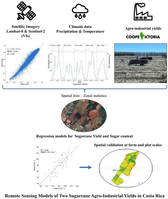
Modelling Two Sugarcane Agro-Industrial Yields Using Sentinel/Landsat Time-Series Data and Their Spatial Validation at Different Scales in Costa Rica

Abstract

Sugarcane production is a relevant socioeconomic activity in Costa Rica that requires tools to improve decision-making, particularly with the advancement of agronomic management using remote sensing (RS) techniques. Some contributions have evaluated sugarcane yield with RS methods, but some gaps remain, such as the lack of operational models for predicting yields and joint estimation with sugar content. Our study is a contribution to this topic that aims to apply an empirical, operational, and robust method to estimate sugarcane yield (SCY) and sugar content (SC) through the combination of field variables, climatic data, and RS vegetation indices (VIs) extracted from Sentinel-2 and Landsat-8 imagery in a cooperative in Costa Rica for four sugarcane harvest cycles (2017–2018 to 2020–2021). Based on linear regression models, four approaches using different VIs were evaluated to obtain the best models to improve the RMSE results and to validate them (using the harvest cycle of 2021–2022) at two management scales: farm and plot. Our results show that the historical yield average, the maximum historical yield, and the growing cycle start were essential factors in estimating SCY and the former variable for SC. For SCY, the most explicative VI was the Simple Ratio (SR), whereas, for SC, it was the Ratio Vegetation Index (RVI). Adding VIs from different months was essential to obtain the phenological variability of sugarcane, being the most common results September, December and January. In SC estimation, precipitation (in May and December) was a clear explicatory variable combined mainly with RVI, whereas in SCY, it was less explanatory. In SCY, RMSE showed values around 8.0 t·ha⁻¹, a clear improvement from 12.9 t·ha⁻¹, which is the average obtained in previous works, whereas in SC, it displayed values below 4.0 kg·t⁻¹. Finally, in SCY, the best validation result was obtained at the plot scale (RMSE of 7.7 t·ha⁻¹), but this outcome was not verified in the case of SC validation because the RMSE was above 4.0 kg·t⁻¹. In conclusion, our operational models try to represent a step forward in using RS techniques to improve sugarcane management at the farm and plot scales in Costa Rica.

1. Introduction

Sugarcane production is an important activity for Costa Rica because it brings economic, labour, social, technological, and even cultural benefits [1]. In 2021, 58,268.6 ha of sugarcane cultivation was reported [2], which the Liga Agrícola Industrial de la Caña de Azúcar (LAICA, the governing body of sugarcane in Costa Rica) divided into six regions. Annually, sugarcane production generates approximately 100,000 jobs, both directly and indirectly, providing an economic contribution to the local economy between 200 and 250 million USD, considering sugar and its derivatives [3].

The sugarcane is a perennial grass growing in the tropical and subtropical world regions with a high concentration of sucrose in the stalk, and it has four phenological stages. In the case of Costa Rica, these stages extend approximately three months, but in other countries, they may change depending on the variety, local conditions, culture management, and geographical parameters [4]. The first stage is seed and germination, characterized by the appearance of buds that allow partial soil coverage with vegetation [5,6]. Next is the stage of tillering and canopy development, where the newly sprouted plants have rapid growth and cover the soil with the crop; after that, the period of great growth begins, when the crop intercepts a high percentage of solar radiation, and the stalk has a fast elongation [7]. Finally, the maturation stage is characterized by an increase in the concentration of sucrose in the stalks and a reduction in the leaf area [8]. Sugarcane fields are harvested several times after the first planting (known as plant crop), and then new ratoons emerge from the same root system [6,9].

The constant interest in increasing sugarcane productivity and its sustainability has promoted the incorporation of remote sensing (RS) in decisions made around crop management due to its repetitive and synoptic coverage and cost-efficient provision [10,11,12]. The principal applications of RS in sugarcane plantations are crop mapping, variety classification, crop growth anomaly, health monitoring, and yield estimation [4,13]. There are some examples of RS applications for sugarcane yield estimation, including in [14], which is one of the first studies that integrated agrometeorological data and spectral information (Ratio Vegetation Index, RVI) from Landsat-4 and 5 in Brazil.

One of the most common RS techniques for sugarcane yield estimation is the use of vegetation indices (VIs) because they are quantitative measurements indicating the vigor of vegetation, and they are easy to obtain [15]. Some studies have found positive relationships between VIs and sugarcane yield. For instance, Rao et al. [16] found positive correlations between the Normalized Difference Vegetation Index (NDVI) and yield using the Indian Remote Sensing Satellite (IRC-1C) and Landsat data in India. Another example of different satellite data combinations (Landsat and ASTER) is found in Almeida et al. [17], in which the authors intended to forecast sugarcane yield using VIs, Principal Component Analysis, and historical harvest data.

Fernandes et al. [18] evaluated the feasibility of estimating yield at the municipality scale using NDVIs extracted from SPOT-Vegetation images with low spatial resolution (1 km²) and meteorological data in Brazil. In contrast, Mutanga et al. [19] used the same images to forecast yield at a regional scale in Zimbabwe. In Kenya, Mulianga et al. [20] showed the difficulty in forecasting the yield on an annual basis using low-resolution satellite images (MODIS) and precipitation data, whereas, in India, Dubey et al. [21] explored an RS-based approach for predicting yield using multiple linear regression, at the district scale, with the Vegetation Condition Index (VCI) and MODIS images, concluding that the relation between VCI and yield was poor in some districts. Another example of the combination of different satellite data, but with more spatial resolution, is Morel et al. [22] in Reunion Islands, where they used an NDVI time series derived from SPOT-4 and SPOT-5 in some farm fields to predict sugarcane yield, where a linear empirical model produced the best results. In Australia, Rahman and Robson [23] combined Landsat and Sentinel images using the same technique to estimate yield at the block level, and in Ethiopia, Abebe et al. [24] merged Landsat and Sentinel images (and different VIs) to estimate yield using a support vector regression, a multilayer perception neuronal network, and a multiple linear regression. Finally, dos Santos Luciano et al. [25] calibrated other predictors to forecast sugarcane yield but only using Landsat satellite images (and different VIs) and agronomic and meteorological data with Random Forest regression.

Recently, a new type of platform, the unmanned aerial vehicle (UAV), has been used to estimate sugarcane yield with high precision in small study areas, such as 3.6 hectares in [26], 5 hectares in [27], 1 hectare in [28], and around 1 hectare in [29]. Images from UAVs are very useful for precision agriculture, given their high spatial resolution (centimeters), among other characteristics, and they are increasingly common in research [30]. Nevertheless, in this study, the application of UAVs was not feasible because our study area was quite extensive, more than 500 ha, and because the time series of VIs were required since 2017, which was impossible to have with UAVs.

In summary, from the mentioned works, the following lessons can be derived. First, the combination of RS images extracted from different sensors is a preferable option for obtaining robust multitemporal series and minimizing the presence of clouds and other artifacts. In addition, the use of several VIs (GNDVI, NDVI, etc.) for analyzing/including the annual phenological evolution is very usual, with a predominance of NDVI. The VIs have been combined with other climatic and agronomic data to improve sugarcane yield estimation. At the same time, a tendency to enhance the spatial resolution has been identified (from VEGETATION to UAV), also affecting the scale of the work, from regional to local. Finally, the most common method for yield estimation has been multivariate linear regression (MLR), which achieves an average root mean square error (RMSE) of 12.9 t·ha⁻¹ [4]. Conversely, one issue or limitation is that most studies have been undertaken at a research level with less operational sugarcane yield-prediction models [4,13]. This situation may be worse in the case of Costa Rica because, in the literature review, an incipient development was observed in models for the estimation of sugarcane yields, including geospatial information [28,31].

In addition to having yield-estimation models with good adjustment parameters, it is necessary to know the spatial variability of yield production inside each crop area to define management strategies, delimit management zones, and understand yield determinants [32]. The operational nature of models will also improve the identification of low-productivity farms and plots as a basis for implementing optimization strategies for the following season, make the planning of harvesting logistics clearer, and verify the reliability of farmers’ pre-harvest estimates [33]. In the context of sugarcane research, many studies have developed a yield-estimation model; however, few have mapped the spatial variability of the model even though that information is very valuable for improving crop management [34]. Another constraint is the low number of works that include both the sugarcane yield estimate (t·ha⁻¹) and the sugar content prediction (kg·t⁻¹), which are important for the sugarcane agro-industry. Indeed, from an economic point of view, the producers are paid based on these indicators. Nevertheless, two exceptions have been observed: Bégué et al. [35] obtained a better relationship between the sugarcane yield and the NDVI acquired before the maturation stage, whereas for sugar content and the NDVI the link was during the maturation stage. Moreover, Shendryk et al. [36] identified that the sugarcane yield and the sugar content can be estimated by integrating satellite variables and climatic data four months before harvest.

The objective of this study was to apply an empirical, operational, and robust method for estimating sugarcane yield and sugar content through the combination of field variables, climatic data, and RS VIs calculated with Sentinel-2 and Landsat-8 satellite images in a producer’s cooperative in Costa Rica and to validate the results at two different scales. The estimation models were adjusted to the reality of the cooperative, which manages heterogeneous farms according to size, agronomic management practices, and agroecological conditions. The contribution of this research is fourfold: (1) to obtain empirical and operational models adapted to the local needs of Costa Rica, combining field variables, historical yield indicators, climatic data, and RS VIs; (2) to fit the best models comparing four approaches—(a) the use of just one specific VI, (b) the combination of different VIs, (c) the merging of just one specific VI and climatic data, and (d) the integration of different VIs and climatic data; (3) to improve the RMSE of models compared with some previous works developed in other countries and related to the traditional estimate of the cooperative based on empirical knowledge; and, finally, (4) to validate the spatial variability of sugarcane yield and sugar content at two different scales: farms and plots.

2. Materials and Methods

2.1. Study Area

Sugarcane production in Costa Rica has been organized through national legislation that has allowed sugarcane production to be divided and organized into six regions with different edaphoclimatic and production characteristics. The regions are Guanacaste, Pacífico Central, Valle Central, Zona Norte, Zona Sur, and Turrialba/Juan Viñas [37,38] (Figure 1b).

The study area is part of the “Valle Central” production region located in the West Central Valley of Costa Rica; it contains the sugarcane plantations of the CoopeVictoria R.L. cooperative (Figure 1c). This region is particularly interesting because it was the first sugarcane production region in Costa Rica, and nowadays, it has strong commercial, industrial, and urban development, increasing the pressure on agricultural lands and producing a decreasing trend in the cropped area [39]. We worked with 26 farms that sum 511 hectares with a mean of 19.6 hectares per farm and with different planted varieties, of which RB86-7515 and LAICA 07-09 were the most common.

The context of the study area is characterized by having soils of the order andisols, inceptisols, and their associations [40]. The study area may be divided into two climatic zones according to the available meteorological stations: the wettest zone, named DIECA (the data from this meteorological station were provided by DIECA (Departamento de Investigación y Extensión de la Caña de Azúcar)), where the rainfall is around 2600 mm and the mean temperature is close to 21.5 °C, and the driest zone, named Argentina (these data were obtained from the Argentina station of the National Meteorological Institute, IMN in Spanish), which has a mean precipitation of about 2000 mm and a mean temperature close to 22.4 °C. Both zones have two climatic seasons: one dry, from December to April, and another rainy, from May to November. Furthermore, there is a slight decrease in rainfall around July, which is known as “Canícula” in Costa Rica [41]. Figure 2 shows that in DIECA, from 2021 to 2022, this climatic phenomenon did not happen, a clear exception in the general precipitation trend.

The average temperature is quite constant throughout the year, oscillating between 20 °C and 25 °C. The 26 studied farms were divided into two groups using a neighborhood criterion based on the available meteorological stations. We assigned 21 farms to the wettest zone (DIECA), and the other 5 farms were included in the driest zone (Argentina). Monthly accumulated precipitation and average temperature data were assigned to each farm according to their closeness to meteorological stations.

2.2. Sugarcane Crop Cycle in Costa Rica

In general, the sugarcane crop cycle in Costa Rica has homogeneous patterns, with each phenological stage lasting approximately ninety days. However, the start time of the growing season varies across regions due to differences in climatic conditions, management culture, or workforce availability (Figure 3). In the regions with irrigation systems, the phenological cycle of new sugarcane planting can start in January, while in other regions without irrigation systems, farmers must wait for the rainy season. The end of the sugarcane crop cycle depends on the start time, but the full cycle generally takes twelve months.

In the “Valle Central” region, the consequence of the local conditions is that the plant is sown between May and June, such that the start of the crop cycle coincides with the rainy season. The maturation stage ends in April of the next year; however, for ratoon plots, the maturation stage starts in January. For ratoons, new plants begin to emerge about fifteen days after harvest, but their growth may be limited by low rainfall and the absence of an irrigation system, which makes it difficult to carry out agronomic practices such as fertilization [43].

2.3. Available Data

2.3.1. Yield and Climatic Data

To model sugarcane estimations of sugarcane yield and sugar content, four harvest seasons were included: 2017–2018, 2018–2019, 2019–2020, and 2020–2021. The data for the two agro-industrial yields were obtained from the cooperative CoopeVictoria R.L. using the total production at the farm scale. Sugarcane yield (t·ha⁻¹) is the sum of the tons of stalks harvested on a specific farm divided by its area in hectares, whereas sugar content (kg·t⁻¹) is the mean of kilograms of sugar that can be obtained from one ton of stalks. The traditional harvesting process is used, which is manual, very labour-intensive, and time-consuming, while the yields are calculated following industrial processes. To validate the best-adjusted estimation models, an additional season was added, corresponding to 2021–2022, from the same source. In this last harvest season, the data were available at two scales: the farm scale and the plot scale (Figure 4). The data at the plot scale allowed validation with an improved spatial resolution, which is very uncommon in sugarcane research. According to production data, during the harvest cycles from 2017–2018 to 2020–2021, this cooperative had a mean sugarcane yield of 88.6 t·ha⁻¹, while the mean sugar content was 119.3 kg·t⁻¹ during the same period. Based on empirical knowledge from the cooperative, the estimated RSME of sugarcane yield for the 2021–2022 harvest cycle was 12.9 t·ha⁻¹.

Harvest yield records have been used to model sugarcane yield based on RS in some works [17,20]. As is known, sugarcane yields decline with successive ratoon crops [44,45], being the knowledge of this decay essential for the modelling of sugarcane yield and sugar content. Therefore, an understanding of their historical trends is required. In this work, historical yield indicators, the historical average yield and the historical maximum yield, were calculated; the former considered the average of the 2015–2016 and 2016–2017 harvest cycles, while the latter retained the maximum yield achieved between those two years, both included as independent variables in the first evaluated harvest season (2017–2018). To more comprehensively explore the historical perspective, the same indicators were aggregated from the previous harvest cycles before the evaluation year for the rest of analysed seasons (2018–2019, 2019–2020, and 2020–2021 yield data). Climatic data were included as independent variables, specifically the accumulated precipitation and average temperature by month, which were obtained from the IMN of Costa Rica and DIECA for 2017 to 2022.

2.3.2. Satellite Images and Vegetation Indexes

In this work, given the high presence of clouds, the combination of two different satellite images, Sentinel and Landsat, was needed, as used in previous studies [35,46,47,48]. Level 2 images from Sentinel-2A and 2B (MSI sensor) were downloaded from European Space Agency (ESA) using the Copernicus Open Access Hub (https://scihub.copernicus.eu/dhus/#/home, accessed on 25 January 2022), and Landsat-8 (OLI sensor) images in level 2 were downloaded from the collection two of the United States Geological Survey (USGS) using the Earth Explorer portal (https://earthexplorer.usgs.gov/, accessed on 25 January 2022). Downloading the images processed in level 2 allowed the use of images with reflectance on the Earth’s surface, reducing the influence of the atmosphere on satellite images. The specific processing chain for both images used different algorithms: Landsat-8 images were processed using the Landsat Surface Reflectance Code (LaSRC) [49], while Sentinel-2 images were treated with the Sen2Cor algorithm [50].

The estimation models for sugarcane yield and sugar content were calibrated with 34 images obtained from 2017–2018 to 2020–2021 (

Table 1. Availability of Landsat-8 (L8) and Sentinel-2 (S2) images in the study area for the five harvest cycles, 2017–2018 to 2021–2022.

Month	Harvest Cycles
	2017–2018	2018–2019	2019–2020	2020–2021	2021–2022
May	L8-2017-05-18	S2-2018-05-11	S2-2019-05-16	L8-2020-05-26	S2-2021-05-15
June	L8-017-06-19	L8-2018-06-22	S2-2019-06-30	ND	S2-2021-06-19
July	S2-2017-07-15	L8-2018-07-24	L8-2019-07-27	ND	L8-2021-07-16
August	L8-2017-08-22	L8-2018-08-25	S2-2019-08-24	S2-2020-08-28	L8-2021-08-17
September	L8-2017-09-07	S2-2018-09-13	S2-2019-09-08	L8-2020-09-15	S2-2021-10-02 *
October	L8-2017-11-10 *	S2-2018-11-07 *	L8-2019-10-31	S2-2020-10-22	ND
November	S2-2017-11-17	L8-2018-11-13	S2-2019-11-22	S2-2020-11-26	S2-2021-11-26
December	S2-2017-12-22	S2-2018-12-27	S2-2019-12-27	S2-2020-12-21	S2-2021-12-31
January	S2-2018-01-26	S2-2019-01-31	S2-2020-01-31	S2-2021-01-30	S2-2022-01-20

ND = no data. * Due to clouds, these images were assigned to the month before to keep the time series as complete as possible.

). Between May and January, one image per month that was as free of clouds as possible (about <25%) was selected. This option was impossible for the images taken in June and July 2020 because they were completely cloudy. This situation also occurred in the images taken in October 2017 and October 2018, for which images were replaced by images from early November, given the availability of other images in mid-November. Further, the images selected for the harvest cycle of 2021–2022 were used to validate the model. In this period, no images for September were available due to high cloudiness. Nevertheless, an image from October 2 was assigned to the month of September to keep the time series as complete as possible.

For each satellite image, eight VIs were calculated that are common in agricultural applications and sugarcane studies with optical satellite images [4,51]. The VIs were the DVI (Difference Vegetation Index), EVI (Enhanced Vegetation Index), GNDVI (Green Normalized Difference Vegetation Index), NDVI (Normalized Difference Vegetation Index), RI (Redness Index), RVI (Ratio Vegetation Index), SAVI (Soil Adjusted Vegetation Index), and SR (Simple Ratio) (

Table 2. Vegetation indexes (VIs) obtained from the satellite images.

Vegetation Index	Equation	Source
DVI	$NIR-Red$	[52]
EVI	$2.5\times \frac{NIR-Red}{(NIR+C_{1}Red-C_{2}Blue+L)}$ $C_1=6,C_2=7.5,L=1$	[53]
GNDVI	$\frac{Green-Red}{Green+Red}$	[54]
NDVI	$\frac{NIR-Red}{NIR+Red}$	[55]
RI	$\frac{Red-Green}{Red+Green}$	[56]
RVI	$\frac{Red}{NIR}$	[57]
SAVI	$\frac{NIR-Red}{\left(NIR+Red+0.5\right)\times (1+0.5)}$	[58]
SR *	$\frac{NIR}{Red}$	[59]

* This has also been defined in the literature as VIN (Vegetation Index Number) or RVI (Ratio Vegetation Index).

) (Figure 4).

Due to the differences in spatial, spectral, and radiometric resolutions between Sentinel-2 and Landsat-8 images, it was necessary to perform harmonization, without modifying the original spatial resolution (10 m and 30 m, respectively), using the VIs from six images for both satellites, corresponding to those images taken on the same day that were also cloud-free: 7 November 2016, 26 January 2017, 2 March 2018, 16 January 2019, 2 December 2019, and 5 January 2021.

After the VIs were calculated for each image, a systematic network of vectorial points (including all the covers: urban, forest, sugarcane, etc.) with a constant separation was overlaid, and then the median value of 36,570 circular polygons, with a radius of 40 m to consider at least a pixel of Landsat (30 m), was extracted to adjust a linear regression model for each VI. After harmonization regressions were applied, our combination of Sentinel-2 and Landsat-8 satellite images allowed us to create a satisfactory time series covering the sugarcane’s phenological stages in monthly intervals.

Finally, although the phenological cycle in Valle Central theoretically begins in May, it was necessary to create an independent variable to show when the phenological cycle started. Given the lack of this specific information, a factor called the “growing cycle start” was included, defined as the ordinal number of the month in which the GNDVI in a farm was higher than 0.2. This threshold was chosen based on the influence that soil has on the first stages of the crop cycle. The first value assigned was 1 for January, and the last was 5 for May.

2.4. Multivariate Statistical Analysis and Spatio-Temporal Validation

In this study, the dependent variables were sugarcane yield and sugar content, while the independent variables included VIs, the historical yield indicators, and the growing cycle start. We applied some MLR to fit the best predictive models using the independent variables. The initial approach was to follow an additive temporal criterion for each VI (namely, just considering a VI, e.g., SR), beginning in May, followed by June, July, and so on until January, and excluding those months and VIs without statistical significance. A second approach was to combine different VIs to analyse if they fitted better at different phenological stages and, therefore, to improve the sugarcane yield and sugar content estimations [60].

After VIs and historical yield indicators were used, in order to improve our models, climatic data were included in a third approach, combining the first option (using just a specific VI) with climatic data, and in a fourth approach, combining the second option (mixing different VIs) with climatic data. The objective was to evaluate the weight of climatic factors (temperature and precipitation) following the additive temporal criterion. The initial hypothesis was to consider the climatic data as important factors for sugarcane yield and sugar content models [36].

The software R (version 4.0.5) on the RStudio environment (version 2023.03.1+446) was used to fit the models using the function lm(). The significant variables (p-value < 0.05) were selected using the stepwise() function and bidirectional selection criteria available in the StepReg package developed by [61]. We evaluated all fitted models for each month using cross-validation with the trainControl() function and the LOOCV (Leave-one out cross-validation) method included in the caret package developed by [62]. Two indicators were used to select the best-adjusted model for each dependent variable: the determination coefficient (R²) and the root mean square error (RMSE).

A fifth year, corresponding to the 2021–2022 harvest cycle, was used to validate our best operational models of sugarcane yield and sugar content. The estimations were performed using a raster model, with a pixel size of 10 m × 10 m for all the variables, where each pixel indicated the estimated value and consequently showed the spatial variability of both dependent variables. Those new rasters were validated on two different scales: the farm scale and the plot scale. Zonal statistics were calculated to extract the average value of sugarcane yield or sugar content using a vector shapefile with the farms and plots of the study area. The data at the plot scale did not cover all the farm fields for various reasons (erroneous values, lack of data, or inconsistencies); 50 was the final number, equivalent to 28% of all plots and 33.4% of the study area. As an initial hypothesis, the validation at the plot scale would give better results than at the farm scale because, at the former, the spatial generalization is lower due to calculating an average from fewer pixels.

3. Results

3.1. Harmonization of Vegetation Indexes and Temporal Phenological Signatures

The harmonization of VIs from Landsat-8 and Sentinel-2 was successful because the R² parameter was almost greater than 0.9. In the four examples shown in Figure 5, the RMSE was also small for each VI, which validated the combined use of both sensors [63].

The growing cycle start presented a high heterogeneity during the study period because, in this cooperative, the harvest calendar runs from February to April of each year, representing an overlap between two harvest cycles, showing a decreasing trend until March and an increasing trend from April onward (Figure 6). During the five harvest cycles analysed, the percentage of farms that began the phenological cycle from February to April varied: in the 2017–2018 cycle, 88% of the farms began the crop cycle between the months indicated, while in the 2018–2019 cycle, it was only 64%, a similar percentage to the 2019–2020 cycle, i.e., 69%, but clearly inferior to the value in 2020–2021, i.e., 91%, and, finally, in the 2021–2022 cycle it was 69%.

A possible cause of the high variability at the beginning of the phenological cycle could be the agronomic management according to the availability of labour or the diverse meteorological conditions. Consequently, the phenological cycle of farms presented great variability in the initial stages and partially in the later ones during the five cycles evaluated. In May, June, and July, the crop presented high variability accompanied by a strong increase in the value of the NDVI, one of the VIs most used in sugarcane research, as previously mentioned.

This period coincides with the beginning of planting and germination when the crop partially covers the ground with leaves. Subsequently, a reduction occurs in the variability of the index accompanied by a relative seasonality between August and December; during this time, the phenological stages of tillering and high growing occur, producing a total ground cover. Finally, in January, there is a reduction in the index accompanied by an increase in the variability. These variations are associated with the final stage of the phenological cycle, the maturation, when a reduction in foliar coverage is shown due to the translocation of assimilates to the stalk [6].

3.2. Sugarcane Yield Models

3.2.1. Modelling Sugarcane Yield at the Farm Scale

The sugarcane yield models were obtained from the first four harvest cycles of 2017–2021.

Table 3. Results of multivariate linear regressions to estimate sugarcane yield (2017–2021, in t·ha⁻¹) per VI (each of them individually, shown in the rows) and per month (from May to January, shown in the columns) after applying the additive temporal criterion and excluding those months and VIs without statistical significance, including historical yield indicators and growing cycle start.

	Month	May	June	July	August	September	October	November	December	January
DVI	R2	*	*	*	*	0.48	0.50	*	*	0.61
	RMSE					10.2	10.1			9.1
EVI	R2	*	*	*	0.48	0.49	*	*	*	*
	RMSE				10.7	10.1
GNDVI	R2	*	*	*	*	*	*	*	0.56	0.56
	RMSE								9.2	9.2
NDVI	R2	*	*	*	*	*	0.53	0.56	0.60	0.63
	RMSE						10.2	9.5	9.0	8.9
RI	R2	*	*	*	0.48	0.55	0.61	0.64	0.64	0.66
	RMSE				10.8	9.4	9.1	8.7	8.7	8.5
RVI	R2	*	*	*	*	0.47	0.53	0.55	0.60	0.60
	RMSE					10.2	10.3	9.6	9.0	9.0
SAVI	R2	*	*	*	*	*	*	*	*	*
	RMSE
SR	R2	*	*	*	0.47	0.53	0.56	0.57	0.65	0.68
	RMSE				10.8	9.9	9.6	9.2	8.4	8.1

* = Without statistical significance (p-value > 0.05). The specific significant independent variables are only shown in Equation (1), equivalent to the best-selected model for sugarcane yield estimation under the first approach. The intensity of the colours is associated with the adjustment of R² and RMSE; darker colours indicate a better fit, while lighter colours suggest a less optimal fit.

shows the R² and RMSE results of the MLR models of sugarcane yield according to the first approach, following the additive temporal criterion for individual VIs (not combined), historical yield indicators, and growing cycle start. This table displays the results for every model per VI (each of them individually, as indicated in the rows) and per month (from May to January, presented in the columns), but without describing the specific significant independent variables. The best-selected model for sugarcane yield under this first approach is shown in Equation (1).

In general, the R² presented a growing trend from September until the maximum in December–January (0.68 with SR, Table 3). The SR and RI indices alternated as the most appropriate to estimate sugarcane yield between September to January, whereas no VI was significant in May, June, and July due to the high heterogeneity in the initial phenological stages of the plantation, as shown in Figure 6. On the other hand, RMSE appeared with a decreasing trend from September until the minimum in December–January (8.1 t·ha⁻¹ with SR). Therefore, after the additive temporal criterion was applied, the best results were obtained, including the SR indices from September, December, and January, as shown in Equation (1), and the rest of the months were not significant. This equation describes the regression model that presented the best results before using the other approaches for the estimation of sugarcane yield (ŷ_SCY), obtaining a model that explained 68% of the variance (R² of 0.68), with an RMSE of 8.1 t·ha⁻¹ (Figure 7a).

$${\mathrm{ŷ}}_{SCY}=35.8+0.8\times A_{SCY}-5.5\times G_{CS}-0.5\times M_{SCY}+3.5\times {SR}_{Sep}+2.3\times {SR}_{Dec}+1.9\times {SR}_{Jan}$$

(1)

where A_SCY is the historical average of sugarcane yield (t·ha⁻¹) on each farm; G_CS indicates the growing cycle start by year; M_SCY indicates the maximum historical sugarcane yield obtained in the farm (from 2015 to 2021); and SR_Sep, SR_Dec, and SR_Jan are the SR indices for September, December, and January, respectively.

The best result after applying the second approach, using the additive temporal criterion and combining different VIs, is shown in Equation (2). The estimation of sugarcane yield (ŷ_SCY), including the average sugarcane yield, the growing cycle start, and the maximum sugarcane yield as significant factors, replaced the SR_Sep and SR_Jan by RI_Sep and DVI_Jan, respectively. This approach reported an R² of 0.69 and an RMSE of 8.1 t·ha⁻¹ (Figure 7b) and, consequently, very similar to Model (1).

$${\mathrm{ŷ}}_{SCY}=43.3+0.6\times A_{SCY}-5.1\times G_{CS}-0.4\times M_{SCY}-135.8\times {RI}_{Sep}+1.5\times {SR}_{Dec}+52.3\times {DVI}_{Jan}$$

(2)

where A_SCY is the historical average of sugarcane yield (t·ha⁻¹) on each farm (from 2015 to 2021); G_CS indicates the growing cycle start by year; M_SCY indicates the maximum historical sugarcane yield obtained on the farm (from 2015 to 2021); and RI_Sep, SR_Dec, and DVI_Jan are the RI for September, the SR for December, and the DVI for January, respectively.

The results from the third approach, combining the first option (using just a specific VI) with climatic data, showed that the best result was exactly the same as obtained in Equation (1). Therefore, neither the temperature nor the precipitation were explicative factors of sugarcane yield, and consequently, no improved equation was obtained. For this reason, an equation for this approach is not presented. On the contrary, the results from the fourth approach, combining the second option (mixing different VIs) with climatic data, showed the best regression model Equation (3). The estimation of sugarcane yield (ŷ_SCY), considering the average sugarcane yield, the growing cycle start, and the maximum sugarcane yield as significant factors, included the RI, the SR, and the precipitation of December. This combination reported an R² of 0.70 and an RMSE of 8.0 t·ha⁻¹ (Figure 7c) and was consequently slightly better than models 1 and 2.

$${\mathrm{ŷ}}_{SCY}=39.8+0.7\times A_{SCY}-4.8\times S_{GC}-0.5\times M_{SCY}-145.3\times {RI}_{Sep}+2.1\times {SR}_{Dec}+1.5\times {SR}_{Jan}+0.05\times P_{Dec}$$

(3)

where A_SCY is the historical average of sugarcane yield (t·ha⁻¹) on each farm (from 2015 to 2021); G_CS indicates the growing cycle start by year; M_SCY indicates the maximum historical sugarcane yield obtained on the farm (from 2015 to 2021); RI_Sep, SR_Dec, and SR_Jan are the RI for September, December, and January, respectively; and P_Dec is the precipitation in December.

Therefore, it was found from the three models that the historical average sugarcane yield (A_SCY) and its maximum historical yield (M_SCY) were significant explanatory factors because the historical trend of the farms reflected the expected potential sugarcane yield (each farm has a maximum threshold that is related to its historical trend). At the same time, the growing cycle start (G_CS) affected the development of the cultivation and the time that the plantation was maintained in the field before being harvested. According to Model (1), SR indexes presented an additive contribution when they were incorporated in September, December, and January. The second model introduces the RI_Sep with a negative weight already being expected, given its formula (Red/NIR) and the DVI_Jan. Finally, if the third model was considered, the influence of the December precipitation was significant.

3.2.2. Spatial Validation of Sugarcane Yield at Farm and Plot Scales

The spatial validation of our three operational regression models to estimate sugarcane yield at the farm scale was carried out using the 2021–2022 harvest cycle. Figure 8a and Figure 7b,c show the three models from Equations (1)–(3), respectively, all with similar R² values (0.66, 0.68, and 0.67, respectively) but with a better RMSE in the first model Equation (1). These figures, compared with Figure 7a–c, showed that the R² was slightly lower and the RMSE was higher, mainly in the second and third models (Figure 8b,c). Therefore, according to the validation process, Equation (1) was considered the best model for sugarcane yield at the farm scale because it had a similar R² but a better RSME than Equations (2) and (3). The main advantage of using this model compared to Equation (3), the best model before validating, is that Equation (1) is “simpler” because it just involves one VI (SR) and no climatic data are needed, which can sometimes be difficult to obtain at the local scale.

The results of the operational regression models for sugarcane yield at plot scale showed quite similar results, with an R² of 0.71 and an RMSE of 7.7 t·ha⁻¹ for Model (1), 0.73 and 7.9 t·ha⁻¹ for Model (2), and 0.71 and 8.6 t·ha⁻¹ for Model (3) (Figure 9a–c, respectively). Therefore, a slightly better validation was obtained at the plot scale compared to the farm scale due to the lower spatial variability that existed in the smallest units, the plots, unlike the farms, where the variability was greater. The same was true in the farm scale validation, where Equation (1) was the best model.

Figure 10 shows our operational regression model from Equation (1) for sugarcane yield estimation in a raster of 10 m × 10 m with the plot boundaries overlaid. In Figure 10a, the spatial variation of yield between the north and the south plots is very clear: the northern farms are more productive than the southern. Figure 10b,c also displays the sugarcane yield variability inside each plot of two farms, improving our spatial estimation compared with the farm scale. For instance, in plot 1, the yield estimation is quite different between the northeast, with higher values (about 130 t·ha⁻¹), and the southwest, with lower values (about 50 t·ha⁻¹).

3.3. Sugar Content Models

3.3.1. Modelling Sugar Content at Farm Scale

The sugar content models were obtained from the first four harvest cycles, 2017–2021.

Table 4. Results of multivariate linear regressions to estimate sugar content (2017–2021, in kg·t⁻¹) per VI (each of them individually, shown in the rows) and per month (from May to January, shown in the columns) after the application of the additive temporal criterion and excluding those months and VIs without statistical significance, including historical yield indicators and growing cycle start.

	Month	May	June	July	August	September	October	November	December	January
DVI	R2	0.29	*	*	*	0.28	0.37	0.37	*	*
	RMSE	6.7				6.3	5.8	6.0
EVI	R2	0.29	*	*	*	0.39	0.39	0.38	0.48	0.49
	RMSE	6.7				5.9	5.8	6.0	5.7	5.8
GNDVI	R2	0.26	*	*	*	0.33	*	*	*	*
	RMSE	6.9				6.1
NDVI	R2	0.28	*	*	*	0.34	0.39	*	*	*
	RMSE	6.8				6.1	5.7
RI	R2	0.29	*	*	*	0.30	0.35	0.34	0.40	0.40
	RMSE	6.7				6.2	5.9	6.1	6.0	6.0
RVI	R2	0.29	*	*	0.27	0.34	0.39	0.46	0.46	0.46
	RMSE	6.8			6.7	6.1	5.8	5.6	5.6	5.6
SAVI	R2	0.29	*	*	*	0.28	0.38	*	*	*
	RMSE	6.7				6.3	5.8
SR	R2	0.28	*	*	*	0.31	0.40	0.48	0.48	0.48
	RMSE	6.8				6.2	5.8	5.6	5.6	5.6

* = Without statistical significance (p-value > 0.05). The specific significant independent variables are only shown in Equation (4), the best-selected model for sugar content estimation under the first approach. The intensity of the colours is associated with the adjustment of R² and RMSE; darker colours indicate a better fit, while lighter colours suggest a less optimal fit.

shows the R² and RMSE results of the MLR models of sugar content according to the first approach, following the additive temporal criterion for individual VIs (not combined), historical yield indicators, and growing cycle start. This table shows the results for every model per VI (each of them individually, indicated in the rows) and per month (from May to January, shown in the columns) but without describing the specific significant independent variables. This information is shown in Equation (4), the best-selected model for sugar content under this first approach.

In general, the R² presented a growing trend from September until the maximum in January (0.49 with EVI, Table 4). The EVI and SR indices were the most appropriate to estimate sugar content between September to January, whereas in May, they were less explicative due to the high heterogeneity in the initial phenological stages of plantation (Figure 6); in June, July, and August, almost all the VIs were not significant. On the other hand, RMSE appeared with a slightly decreasing trend from September until the minimum in January (5.6 kg·t⁻¹ with SR). Therefore, after the additive temporal criterion was applied, the best results were obtained, including EVI indices from August, September, November, and January, as shown in Equation (4), where the rest of the months were not significant. This equation describes the best regression model before applying the other approaches, being a model that explained 49% of the variance (R² of 0.49) with an RMSE of 5.8 kg·t⁻¹ (Figure 11a).

$${\mathrm{ŷ}}_{SC}=40.6+0.6\times A_{SC}-56.2\times {EVI}_{Aug}+87.4\times {EVI}_{Sep}-41.8\times {EVI}_{Nov}+29.0\times {EVI}_{Jan}$$

(4)

where A_SC is the historical average of sugar content (kg·t⁻¹) on each farm, and EVI_Aug, EVI_Sep, EVI_Nov, and EVI_Jan are the EVI for August, September, November, and January, respectively.

On the other hand, the best result after applying the second approach, to use the additive temporal criterion and to combine different VIs, is shown in Equation (5). The estimation of sugar content (ŷ_SC), including the average sugar content and the combination of SR and GNDVI, reported an R² of 0.59 and an RMSE of 5.0 kg·t⁻¹ (Figure 11b) and was consequently a bit better than Model (4).

$${\mathrm{ŷ}}_{SC}=-61.9+0.5\times A_{SC}-1.2\times {SR}_{Aug}+81.1\times {GNDVI}_{Sep}+106.6\times {GNDVI}_{Nov}$$

(5)

where A_SC is the historical average of sugar content (kg·t⁻¹) on each farm (from 2015 to 2021) and SR_Aug, GNDVI_Sep, and GNDVI_Nov are the SR for August, the GNDVI for September, and the SR for November, respectively.

The third approach for sugar content estimation at the farm scale, combining the first option (using just a specific VI) with climatic data, showed an improvement in the model, contrary to what was obtained in the sugarcane yield. The estimation of sugar content (ŷ_SC), including the average of sugar content with the joint of RVI and precipitation, reported an R² of 0.77 and an RMSE of 3.9 kg·t⁻¹ (Figure 11c) and was consequently the best model compared with Equations (4) and (5).

$${\mathrm{ŷ}}_{SC}=64.74+0.67\times A_{SC}-53.9\times {RVI}_{Nov}-16.7\times {RVI}_{Jan}-0.03\times P_{May}-0.09\times P_{Dec}$$

(6)

where A_SC is the historical average of sugar content (kg·t⁻¹) on each farm (from 2015 to 2021), RVI_Nov and RVI_Jan are the RVI for November and January, and P_May and P_Dec are the precipitation of May and December.

Finally, after temperature and precipitation were added, a seventh regression model was obtained Equation (7), corresponding to the fourth approach. The estimation of sugar content (ŷ_SC), including the historical average sugar content with the combination of SR and GNDVI and precipitation, reported an R² of 0.77 and an RMSE of 3.8 kg·t⁻¹ (Figure 11d) and was consequently a better model compared with models (4) and (5), but very similar to Model (6).

$${\mathrm{ŷ}}_{SC}=38.2+0.6\times A_{SC}+25.4\times {GNDVI}_{Sep}+1.6\times {SR}_{Jan}-0.02\times P_{May}-0.09\times P_{Dec}$$

(7)

where A_SC is the historical average of sugar content (kg·t⁻¹) on each farm (from 2015 to 2021); GNDVI_Sep and SR_Jan are the GNDVI VI for September, SR is the VI for January, and P_May and P_Dec are the precipitation of May and December.

Therefore, it was found from the four models that the historical average of sugar content (A_SCY) was an essential explanatory factor in estimating sugar content because it reflected the expected potential content, as it happened with the models to estimate sugarcane yield. According to Model (4), EVI indices presented an additive contribution when they were incorporated in different months, i.e., August, September, November, and January, whereas the fifth model introduced the combination of SR_Aug, GNDVI_Sep, and GNDVI_Nov. The sixth model considered RVI_Nov and RVI_Jan and the precipitation of May and December, while the last model involved the influence of GNDVI_Sep and SR_Jan and the precipitation of May and December as significant factors.

3.3.2. Spatial Validation of Sugar Content at Farm and Plot Scales

The spatial validation of our four operational regression models to estimate sugar content on the farm scale was performed in the same way as for sugarcane yield, using the 2021–2022 harvest cycle data. Figure 12a–d show the four models from Equations (4)–(7), respectively, all displaying a similar R² (0.59, 0.58, 0.56, and 0.57, respectively) but a better RMSE in the sixth model Equation (6). These figures, compared with Figure 11a–d, showed that the R² was better in Model (4), similar to Model (5), and lower in Models (6) and (7). The RMSE was lower in the fourth and sixth models but higher in the fifth and seventh. Therefore, Equation (6) was considered the best model for sugar content because, although it had a similar R², the RMSE was clearly better. The main advantage of using this model compared with the others is that it uses only one VI (RVI) combined with precipitation.

The results of the operational regression models for sugar content at the plot scale showed an R² of 0.45 and an RMSE of 6.8 kg·t⁻¹ from Equation (4), 0.43 and 11.3 kg·t⁻¹ from Equation (5), 0.46 and 4.7 kg·t⁻¹ from Equation (6), and 0.49 and 4.9 kg·t⁻¹ from Equation (7) (Figure 13a–d). A clearly worse sugar content validation was obtained at the plot scale compared with the farm scale, mainly in Models (4) and (5). Like the validation obtained at the farm scale, Equation (6) followed being the best model.

Based on Equation (6), Figure 14 shows our operational regression model for sugar content estimation in a raster of 10 m × 10 m, with the plot boundaries overlaid. The spatial distribution of sugar content across the study area (Figure 14a) was similar to that obtained for sugarcane yield: the northern farms were more productive than the southern farms. Figure 14b,c also displays the sugar content variability inside each plot of the two farms, showing that the spatial variation was clearly lower compared with the sugarcane yield, probably because of the smaller spatial variability of the independent variables used in Equation (6).

4. Discussion

Combining different satellite images (Landsat and Sentinel) is unavoidable to obtain robust results on regions with high cloudiness during some months of the year [4]. In this work, VIs from Sentinel and Landsat images were harmonized to fill the gaps in a monthly time series and to improve our estimation models because, as [23,24] asserted, the combination of different satellite images produces better results.

Based on linear empirical regressions, our three (in fact, four, but one was not included) operational sugarcane yield models at the farm scale produced similar R² and RMSE results, whereas the spatial validation presented a few smaller R² values in all the models, demonstrating that the best RMSE value is in Model (1). The spatial validation at the plot scale showed similar R² results for all the models but higher than those obtained at the farm scale, whereas the best RMSE followed being in Model (1).

Therefore, in conclusion, our results showed quite similar outputs for sugarcane yield using the three models and two spatial scales, with R² values around 0.7 and RMSEs about 8.0 t·ha⁻¹. However, the first model was shown to be the most constant during the modelling and validating steps, and consequently, including only the SR in different months (September, December, and January) makes it possible to obtain a robust estimation.

Multivariate linear regression has been a common technique to estimate sugarcane yield that has produced promising results given that it can be easily applied to different spatial scales and can combine some explanatory variables from different data sources such as RS, agronomic, and climatic data. For instance, Morel et al. [22] developed an NDVI time series combined with climatic data to predict sugarcane yield and obtained a linear empirical model that produced the best results, with an R² of 0.64 and an RMSE of 10.4 t·ha⁻¹. Also, according to the review by Som-Ard et al. [4], it is the most common yield-estimation method, achieving an RMSE of 12.9 t·ha⁻¹ on average. In our work, and as one of the main objectives, the RMSE values of the models were improved, with values around 8.0 t·ha⁻¹. Two possible reasons for this improvement could be the consideration of the local peculiarities of sugarcane’s temporal phenological signature in Costa Rica through VIs and the inclusion of explicative factors that comprise historic crop management extracted from the Cooperative data.

Our four operational sugar content models at the farm scale produced less similar R² and RMSE results than in sugarcane yield, and the models including precipitation Equations (6) and (7) were better, whereas the spatial validation presented similar R² values in all the models, although the best RMSE was obtained in Model 6. The spatial validation at the plot scale showed a few lower R² and RMSE indicators compared with the validation at the farm scale. The best R² values were obtained in Models 6 and 7, and the best RMSE values were obtained in Model 6. Therefore, our results showed that the model estimation of sugar content was good enough at the farm scale, combining VIs and precipitation data, with an RMSE below 5.0 kg·t⁻¹ in the sixth and seventh models but worse R² and the RMSE values at the plot scale. This outcome rules out this work’s hypothesis that the validation at the plot scale would give better results than at the farm scale because, at the former scale, the spatial generalisation is lower as a result of calculating an average from fewer pixels. One possible explanation for this issue could be the harvest calendar. Those plots harvested at the beginning of the season have less sugar content concentration than those harvested at the end of the season. This fact could be an important source of error at this detailed scale, which is a concern to analyse in future work.

In sugarcane yield modelling, researchers have used diverse VIs, but in our work, the most explanatory was the most simple, which agrees with [14] because they concluded that the ratio of the reflectance of the NIR band by the Red band (NIR/RED: Ratio Vegetation Index (RVI) or Simple Ratio (SR) in our study) is the best index to relate spectral data and observed sugarcane yield. In the same manuscript, they cited the recommendation made by Jackson et al. (1983) of using this index when the crop covers more than 50% of the soil. On the other hand, Abebe et al. [24] mentioned that the GNDVI, SR, NDVI, and SIRI (Short Wave Infrared Ratio) were strongly correlated with sugarcane yield, the GNDVI being the most accurate, reducing the effects of saturation. But, in fact, according to [60], VIs show variations in the amount of vegetation sensitivity at different development stages of crops. Depending on the stage in which the crop is analysed throughout the cycle, there will be a more adequate VI with a higher relationship with vegetation density, green leaf biomass, and leaf area index. Therefore, an important concern to consider is crop stage dynamics and the best time to predict sugarcane yield and sugar content, considering crop phenology. For instance, in refs. [19,35], the authors asserted that the best acquisition period of satellite images for the assessment of sugarcane yield was two months preceding the beginning of harvest, when all the fields were fully developed but before the maturation stage. In our work, September, December, and January were the months of VIs that allowed us to obtain the best-fitting model for sugarcane yield, whereas September, November, and January were the best for models of sugar content. Therefore, our results agree with [36], who identified that the sugar content could be estimated with the integration of satellite variables and climatic data four months before harvest, and with [35], who observed a relationship between the field NDVI acquired during the maturation stage and sugar content in the stalk.

In the combination of different sources for sugarcane yield characteristic of this work, six independent variables were recurrent to the four applied models, two extracted from our modification of the Cooperative records (the historical yield average and the maximum historical yield) and four from VIs (the growing cycle start and the VIs of September, December, and January). The inclusion of the historical indicators was essential for obtaining acceptable results, together with the mentioned variables extracted from VIs. The historical yield average and the maximum historical yield (with negative coefficient) contain the potential of the farm according to historical data (higher maximum historical yields produce less sugarcane yields in the future given the ratoon decline, as reported by [44,45]) as an indication of farm depletion. In contrast, the growing cycle start (with a negative coefficient) includes the time of the plant to fulfil the phenological development.

An essential difference between the best sugar content model and the best sugarcane yield model was that only one common explanatory variable appeared, the historical average of sugar content, being a possible explanation that the farm depletion, extracted from the maximum historical yield, produces a decrease in sugarcane yield but not necessarily a reduction in sugar content. Another main difference was that the SR index, which is very important for sugarcane yield estimation, was less determinant for the estimation of sugar content, sharing its importance with RVI and GNDVI in the best model Equations (6) and (7). For the sixth sugar content model, which was the best from the validation, the RVI of November and January were significant factors, highlighting the dominance of Red and NIR bands as in the case of SR.

According to our results, the temperature was not a predictor factor in any model, whereas precipitation was more frequent as an explicatory variable for sugar content models (mainly evidenced in Equations (6) and (7) from May and December, with negative regression coefficients), which may be due to the stronger inverse relationship than the precipitation has with the sugar content in the last months of the sugarcane cycle when the maturation stage naturally starts in a hybrid stress condition. In this sense, the negative coefficient of the December precipitation is because, during the maturation stage, with a fully developed canopy, the leaves senesce and turn yellowish, corresponding to a water loss in the plant and an increase in the sugar content of the stalk juice [35].

Our modelling approach to assess the spatial variability of sugarcane yield and sugar content at the farm and plot scales allowed us to understand the spatial distribution of both variables mapped. These maps are a new tool for decision-making in this cooperative because they permit a deeper understanding of the within-field variability, delimit management zones, and improve site-specific management strategies. In fact, they may be a good alternative to mapping the spatial variability inside the farms when the harvest activities (the cutting) are manual instead of using mechanical harvesters, as in our case, hindering the data availability with higher spatial density [34].

Finally, according to our results, MLR has produced robust outcomes for two agro-industrial yields during five years and at two different spatial scales. Although the comparison may be complicated, given the different number of farms or plots and of predictors together with pixel sizes involved in the models, other previous works asserted linear relationships between yields and explicative variables, as in the cases of Bégué et al. [35], Morel et al. [22], and Akbarian et al. [29], with linear correlations and R² above 0.6. According to some authors, an alternative technique to MLR for predicting sugarcane yields can be machine learning (ML) approaches. Concretely, they asserted that Random Forest (RF), which is a non-parametric method, is more accurate to estimate yields when sample plots and variation are relatively large. For instance, Canata et al. [34] used filtered and interpolated yield data generated by harvesters at the field level for two years to conclude that RF performed better than MLR in predicting sugarcane yield. Additionally, in opposition to our outputs, they found better results when using the spectral bands directly rather than involving VIs. Dos Santos Luciano et al. [25] also applied an RF algorithm to forecast sugarcane yield and obtained an RMSE a little worse than ours (9.4 t·ha⁻¹ versus 8.0 t·ha⁻¹).

In the case of Shendryk et al. [36], given that harvester operators often do not know the exact boundaries of each field, leading to harvested sugarcane being mixed with that from adjacent fields, small fields (<0.64 ha) were removed. This fact and the large number of predictive variables included (371) in four decision tree-based machine learning algorithms (Random Forest, Gradient Boosting, Extreme Trees, and Extreme Gradient Boosting) were some of the most important differences with our methodology. Their results agree with our assertion that Sentinel-2-derived spectral indices were the most important in predicting sugarcane yield, and climate variables were the most important for predicting sugar yield (sugar content in our work). In contrast, in their prediction model, the RSME was worse compared with our results, with a value of 16 t·ha⁻¹. Therefore, in spite of the benefits and advances of ML reported by other authors, more research is required because the differences in accuracy between ML and linear regression were not always of practical significance, which stresses the importance of proper model calibration and selection [64].

5. Conclusions

In this research, some models based on MLR have been applied to estimate sugarcane yield and sugar content in one cooperative in Costa Rica. The objective was to apply some empirical and operationally robust frameworks for estimating sugarcane yield and sugar content through the combination of different data sources, highlighting the contribution of RS. At the same time, the combined analysis of both parameters tries to provide better knowledge of the sugarcane agro-industry, given the small number of works that include them, mainly in Costa Rica.

The specific contributions of this work were fourfold. The first contribution was the application of operational models adapted to the local conditions (management and climate) of Costa Rica, combining different data sources. Two historical yield indicators, the historical yield average and the maximum historical yield, were essential factors in explaining sugarcane yield, and the former was also essential for explaining sugar content. Other important explicative variables were those provided by RS, where the growing cycles start and VIs were essential.

Second, four approaches using different VIs were evaluated to obtain the best models. In sugarcane yield, one of the most explicatory VI was SR in different months of the growing cycle and with a smaller weight of RI, whereas in sugar content, the most important VI was the RVI and, with a smaller influence, the GNDVI and the SR. The addition of VIs from different months was essential to obtain the phenological variability of sugarcane, which was the most common result considered from September to January. In the estimation of sugar content, precipitation (May and December) was a clear predictor variable, as hypothesized, combined mainly with RVI, whereas in sugarcane yield, it was clearly less explanatory.

In this work, the RMSE values of models were improved as the third contribution, compared with other research developed in other countries and compared with the traditional estimate of the cooperative based on empirical knowledge. Our results showed RMSEs for sugarcane yield around 8.0 t·ha⁻¹, a clear improvement from 12.9 t·ha⁻¹ on average obtained in previous works, where sugar content displayed values below 4.0 kg·t⁻¹.

The fourth contribution was the spatial validation of sugarcane yield and sugar content at two different scales: farms and plots. In terms of sugarcane yield, the best validation result was obtained at the plot scale (RMSE of 7.7 t·ha⁻¹), as hypothesized, given the lower spatial generalisation, because the average was calculated from fewer pixels. Nevertheless, this outcome was not verified in the case of sugar content validation because the RMSE was around 5.0 kg·t⁻¹.

Finally, future work will comprise the application of our operational models for sugarcane yield and sugar content in other Costa Rican regions with larger areas and different management systems. A second future task will be to insert our operational models into a decision support system based on RS, a process currently in development. A third new approach will be the application of alternative algorithms, such as machine learning, to estimate the two agro-industrial yields.

References

1. Angulo, Á.; Rodríguez, M.; Chaves, M. Guía Técnica Cultivo Caña De Azúcar Región: Guanacaste. Available online: https://servicios.laica.co.cr/laica-cv-biblioteca/index.php/Library/download/jieyzwRDmVvUeWJGLRfYLzXbibjfLZNW (accessed on 18 April 2023).
2. INEC (Instituto Nacional de Estadística y Censos). Encuesta Nacional Agropecuaria 2021 Resultados Generales de La Actividad Agrícola y Forestal. Available online: https://inec.cr/estadisticas-fuentes/encuestas/encuesta-nacional-agropecuaria?page=3 (accessed on 18 April 2023).
3. Chaves, M.; Bermúdez, L. Agroindustria Azucarera Costarricense: Un Modelo Organizacional y Productivo Efectivo Con 75 Años de Vigencia. Available online: https://servicios.laica.co.cr/laica-cv-biblioteca/index.php/Library/download/DSCmSdyqoIJhQAUmeqVMAwOPjrySXJdh (accessed on 1 September 2021).
4. Som-Ard, J.; Atzberger, C.; Izquierdo-Verdiguier, E.; Vuolo, F.; Immitzer, M. Remote Sensing Applications in Sugarcane Cultivation: A Review. Remote Sens. 2021, 13, 4040. [Google Scholar] [CrossRef]
5. Allison, J.C.S.; Pammenter, N.W.; Haslam, R.J. Why Does Sugarcane (Saccharum Sp. Hybrid) Grow Slowly? S. Afr. J. Bot. 2007, 73, 546–551. [Google Scholar] [CrossRef]
6. Cock, J.H. Sugarcane Growth and Development. Int. Sugar J. 2003, 105, 540–552. [Google Scholar]
7. Inman-Bamber, N.G. Temperature and Seasonal Effects on Canopy Development and Light Interception of Sugarcane. Field Crop. Res. 1994, 36, 41–51. [Google Scholar] [CrossRef]
8. Saez, J.V. Dinámica de Acumulación de Sacarosa en Tallos de Caña de Azúcar (Saccharum spp.) Modulada por Cambios en la Relación Fuente-Destino. Ph.D. Thesis, Facultad de Ciencias Agropecuarias, Universidad Nacional de Cordoba, 2017. Available online: http://hdl.handle.net/11086/6836 (accessed on 3 December 2020).
9. Molijn, R.A.; Iannini, L.; Rocha, J.V.; Hanssen, R.F. Sugarcane Productivity Mapping through C-Band and L-Band SAR and Optical Satellite Imagery. Remote Sens. 2019, 11, 1109. [Google Scholar] [CrossRef]
10. Pinter, P.J.; Hatfield, J.L.; Schepers, J.S.; Barnes, E.M.; Moran, M.S.; Daughtry, C.S.; Upchurch, D.R. Remote Sensing for Site-Specific Crop Management. Photogramm. Eng. Remote Sens. 2003, 69, 647–664. [Google Scholar] [CrossRef]
11. Liaghat, S.; Balasundram, S.K. A Review: The Role of Remote Sensing in Precision Agriculture. Am. J. Agric. Biol. Sci. 2010, 5, 50–55. [Google Scholar] [CrossRef]
12. Segarra, J.; Buchaillot, M.L.; Araus, J.L.; Kefauver, S.C. Remote Sensing for Precision Agriculture: Sentinel-2 Improved Features and Applications. Agronomy 2020, 10, 641. [Google Scholar] [CrossRef]
13. Abdel-Rahman, E.M.; Ahmed, F.B. The Application of Remote Sensing Techniques to Sugarcane (Saccharum spp. Hybrid) Production: A Review of the Literature. Int. J. Remote Sens. 2008, 29, 3753–3767. [Google Scholar] [CrossRef]
14. Rudorff, B.F.T.; Batista, G.T. Yield Estimation of Sugarcane Based on Agrometeorological-Spectral Models. Remote Sens. Environ. 1990, 33, 183–192. [Google Scholar] [CrossRef]
15. Bannari, A.; Morin, D.; Bonn, F.; Huete, A.R. A Review of Vegetation Indices. Remote Sens. Rev. 1995, 13, 95–120. [Google Scholar] [CrossRef]
16. Rao, P.V.K.; Rao, V.V.; Venkataratnam, L. Remote Sensing: A Technology for Assessment of Sugarcane Crop Acreage and Yield. Sugar Technol. 2002, 4, 97–101. [Google Scholar] [CrossRef]
17. Almeida, T.I.R.; De Souza Filho, C.R.; Rossetto, R. ASTER and Landsat ETM+ Images Applied to Sugarcane Yield Forecast. Int. J. Remote Sens. 2006, 27, 4057–4069. [Google Scholar] [CrossRef]
18. Fernandes, J.L.; Rocha, J.V.; Lamparelli, R.A.C. Sugarcane Yield Estimates Using Time Series Analysis of Spot Vegetation Images. Sci. Agric. 2011, 68, 139–146. [Google Scholar] [CrossRef]
19. Mutanga, S.; van Schoor, C.; Olorunju, P.L.; Gonah, T.; Ramoelo, A. Determining the Best Optimum Time for Predicting Sugarcane Yield Using Hyper-Temporal Satellite Imagery. Adv. Remote Sens. 2013, 2, 269–275. [Google Scholar] [CrossRef]
20. Mulianga, B.; Bégué, A.; Simoes, M.; Todoroff, P. Forecasting Regional Sugarcane Yield Based on Time Integral and Spatial Aggregation of MODIS NDVI. Remote Sens. 2013, 5, 2184–2199. [Google Scholar] [CrossRef]
21. Dubey, S.K.; Gavli, A.S.; Yadav, S.K.; Sehgal, S.; Ray, S.S. Remote Sensing-Based Yield Forecasting for Sugarcane (Saccharum officinarum L.) Crop in India. J. Indian Soc. Remote Sens. 2018, 46, 1823–1833. [Google Scholar] [CrossRef]
22. Morel, J.; Todoroff, P.; Bégué, A.; Bury, A.; Martiné, J.F.; Petit, M. Toward a Satellite-Based System of Sugarcane Yield Estimation and Forecasting in Smallholder Farming Conditions: A Case Study on Reunion Island. Remote Sens. 2014, 6, 6620–6635. [Google Scholar] [CrossRef]
23. Rahman, M.M.; Robson, A. Integrating Landsat-8 and Sentinel-2 Time Series Data for Yield Prediction of Sugarcane Crops at the Block Level. Remote Sens. 2020, 12, 1313. [Google Scholar] [CrossRef]
24. Abebe, G.; Tadesse, T.; Gessesse, B. Combined Use of Landsat 8 and Sentinel 2A Imagery for Improved Sugarcane Yield Estimation in Wonji-Shoa, Ethiopia. J. Indian Soc. Remote Sens. 2022, 50, 143–157. [Google Scholar] [CrossRef]
25. dos Santos Luciano, A.C.; Picoli, M.C.A.; Duft, D.G.; Rocha, J.V.; Leal, M.R.L.V.; le Maire, G. Empirical Model for Forecasting Sugarcane Yield on a Local Scale in Brazil Using Landsat Imagery and Random Forest Algorithm. Comput. Electron. Agric. 2021, 184, 106063. [Google Scholar] [CrossRef]
26. Som-ard, J.; Hossain, M.D.; Ninsawat, S.; Veerachitt, V. Pre-Harvest Sugarcane Yield Estimation Using UAV-Based RGB Images and Ground Observation. Sugar Technol. 2018, 20, 645–657. [Google Scholar] [CrossRef]
27. Sumesh, K.C.; Ninsawat, S.; Som-ard, J. Integration of RGB-Based Vegetation Index, Crop Surface Model and Object-Based Image Analysis Approach for Sugarcane Yield Estimation Using Unmanned Aerial Vehicle. Comput. Electron. Agric. 2021, 180, 105903. [Google Scholar] [CrossRef]
28. Alemán-Montes, B.; Henríquez-Henríquez, C.; Ramírez-Rodríguez, T.; Largaespada-Zelaya, K. Estimación de Rendimiento En El Cultivo de Caña de Azúcar (Saccharum officinarum) a Partir de Fotogrametría Con Vehículos Aéreos No Tripulados (VANT). Agron. Costarric. 2021, 45, 67–80. [Google Scholar] [CrossRef]
29. Akbarian, S.; Xu, C.; Wang, W.; Ginns, S.; Lim, S. Sugarcane Yields Prediction at the Row Level Using a Novel Cross-Validation Approach to Multi-Year Multispectral Images. Comput. Electron. Agric. 2022, 198, 107024. [Google Scholar] [CrossRef]
30. Barbosa Júnior, M.R.; Moreira, B.R.d.A.; de Brito Filho, A.L.; Tedesco, D.; Shiratsuchi, L.S.; da Silva, R.P. UAVs to Monitor and Manage Sugarcane: Integrative Review. Agronomy 2022, 12, 661. [Google Scholar] [CrossRef]
31. Hidalgo, N. Análisis del Rendimiento del Cultivo de Caña de Azúcar Mediante Índices de Vegetación y Monitores de Rendimiento Durante el Periodo de Zafra 2021–2022 en la Empresa Central Azucarera Tempisque S.A. (CATSA) Guanacaste, Costa Rica. Licenciature’s Thesis, Escuela de Ingeniería Agrícola, Instituto Tecnológico de Costa Rica, 2022. Available online: https://repositoriotec.tec.ac.cr/handle/2238/13994 (accessed on 25 April 2023).
32. Jeffries, G.R.; Griffin, T.S.; Fleisher, D.H.; Naumova, E.N.; Koch, M.; Wardlow, B.D. Mapping Sub-Field Maize Yields in Nebraska, USA by Combining Remote Sensing Imagery, Crop Simulation Models, and Machine Learning. Precis. Agric. 2020, 21, 678–694. [Google Scholar] [CrossRef]
33. Dimov, D.; Uhl, J.H.; Löw, F.; Seboka, G.N. Sugarcane Yield Estimation through Remote Sensing Time Series and Phenology Metrics. Smart Agric. Technol. 2022, 2, 100046. [Google Scholar] [CrossRef]
34. Canata, T.F.; Wei, M.C.F.; Maldaner, L.F.; Molin, J.P. Sugarcane Yield Mapping Using High-Resolution Imagery Data and Machine Learning Technique. Remote Sens. 2021, 13, 232. [Google Scholar] [CrossRef]
35. Bégué, A.; Lebourgeois, V.; Bappel, E.; Todoroff, P.; Pellegrino, A.; Baillarin, F.; Siegmund, B. Spatio-Temporal Variability of Sugarcane Fields and Recommendations for Yield Forecast Using NDVI. Int. J. Remote Sens. 2010, 31, 5391–5407. [Google Scholar] [CrossRef]
36. Shendryk, Y.; Davy, R.; Thorburn, P. Integrating Satellite Imagery and Environmental Data to Predict Field-Level Cane and Sugar Yields in Australia Using Machine Learning. Field Crop. Res. 2021, 260, 107984. [Google Scholar] [CrossRef]
37. LAICA Ley Orgánica de La Agricultura e Industria de La Caña de Azúcar N° 7818 Del 22 de Setiembre de 1998. Available online: http://www.pgrweb.go.cr/scij/Busqueda/Normativa/Normas/nrm_texto_completo.aspx?param2=NRTC&nValor1=1&nValor2=44897&strTipM=TC (accessed on 8 May 2023).
38. Montenegro Ballestero, J.; Chaves Solera, M. Análisis de Ciclo de Vida Para La Producción Primaria de Caña de Azúcar En Seis Regiones de Costa Rica. Rev. Ciencias Ambient. 2022, 56, 96–119. [Google Scholar] [CrossRef]
39. Chaves, M.; Chavarría, E. Estimación Del Área Sembrada Con Caña de Azúcar En Costa Rica Según Región Productora. Periodo 1985–2020 (36 Zafras). Available online: https://laica.cr/wp-content/uploads/2022/05/revista-entre-caneros-no22.pdf (accessed on 8 May 2023).
40. Mata, R.; Rosales, A.; Sandoval, D.; Vindas, E.; Alemán, B. Subórdenes de Suelos de Costa Rica [Mapa Digital]. Escala 1:200000. Available online: http://www.cia.ucr.ac.cr/es/mapa-de-suelos-de-costa-rica (accessed on 30 September 2022).
41. Alfaro, E.J. Caracterización del “Veranillo” en dos Cuencas de la Vertiente Del Pacífico de Costa Rica, América Central. Rev. Biol. Trop. 2014, 62, 1–15. [Google Scholar] [CrossRef]
42. Vignola, R.; Poveda, K.; Watler, W.; Vargas, A.; Berrocal, Á. Cultivo de Caña de Azúcar En Costa Rica. Available online: https://www.mag.go.cr/bibliotecavirtual/F01-8327.pdf (accessed on 8 May 2023).
43. Chaves, M. Suelos, Nutrición y Fertilización de la Caña de Azúcar en Costa Rica. Available online: https://servicios.laica.co.cr/laica-cv-biblioteca/index.php/Library/download/xznuAsbXHGPzjuDRWFDDwEOtAUrWraua (accessed on 8 May 2023).
44. Ramburan, S.; Wettergreen, T.; Berry, S.D.; Shongwe, B. Effects of Variety, Environment and Management on Sugarcane Ratoon Yield Decline. Int. Sugar J. 2012, 85, 180–192. [Google Scholar]
45. Dlamini, N.E.; Zhou, M. Soils and Seasons Effect on Sugarcane Ratoon Yield. Field Crop. Res. 2022, 284, 108588. [Google Scholar] [CrossRef]
46. Panigrahy, S.; Sharma, S.A. Mapping of Crop Rotation Using Multidate Indian Remote Sensing Satellite Digital Data. ISPRS J. Photogramm. Remote Sens. 1997, 52, 85–91. [Google Scholar] [CrossRef]
47. Zhao, Y.; Della Justina, D.; Kazama, Y.; Rocha, J.V.; Graziano, P.S.; Lamparelli, R.A.C. Dynamics Modeling for Sugar Cane Sucrose Estimation Using Time Series Satellite Imagery. In Remote Sensing for Agriculture, Ecosystems, and Hydrology XVIII; Neale, C.M.U., Maltese, A., Eds.; SPIE: Bellingham, WA, USA, 2016; Volume 9998, p. 99980J. [Google Scholar]
48. Chaves, M.; Picoli, M.; Sanches, I. Recent Applications of Landsat 8/OLI and Sentinel-2/MSI for Land Use and Land Cover Mapping: A Systematic Review. Remote Sens. 2020, 12, 3062. [Google Scholar] [CrossRef]
49. USGS (United States Geological Survey). Landsat 8-9 Collection 2 (C2) Level 2 Science Product (L2SP) Guide. Available online: https://www.usgs.gov/media/files/landsat-8-9-collection-2-level-2-science-product-guide (accessed on 28 September 2022).
50. Mueller-Wilm, U.; Devignot, O.; Pessiot, L. Sen2Cor Configuration and User Manual. Available online: http://step.esa.int/thirdparties/sen2cor/2.3.0/[L2A-SUM] S2-PDGS-MPC-L2A-SUM [2.3.0].pdf (accessed on 30 June 2023).
51. Jiménez-Jiménez, S.I.; Marcial-Pablo, M.d.J.; Ojeda-Bustamante, W.; Sifuentes-Ibarra, E.; Inzunza-Ibarra, M.A.; Sánchez-Cohen, I. VICAL: Global Calculator to Estimate Vegetation Indices for Agricultural Areas with Landsat and Sentinel-2 Data. Agronomy 2022, 12, 1518. [Google Scholar] [CrossRef]
52. Richardson, A.J.; Wiegand, C.L. Distinguishing Vegetation from Soil Background Information. Photogramm. Eng. Remote Sens. 1977, 43, 1541–1552. [Google Scholar]
53. Huete, A.; Didan, K.; Miura, T.; Rodriguez, E.P.; Gao, X.; Ferreira, L.G. Overview of the Radiometric and Biophysical Performance of the MODIS Vegetation Indices. Remote Sens. Environ. 2002, 83, 195–213. [Google Scholar] [CrossRef]
54. Gitelson, A.A.; Kaufman, Y.J.; Merzlyak, M.N. Use of a Green Channel in Remote Sensing of Global Vegetation from EOS- MODIS. Remote Sens. Environ. 1996, 58, 289–298. [Google Scholar] [CrossRef]
55. Rouse, J.W.; Hass, R.H.; Schell, J.A.; Deering, D.W. Monitoring Vegetation Systems in the Great Plains with ERTS. In Proceedings of the Third Earth Resources Technology Satellite (ERTS) Symposium, Washington, DC, USA, 10–14 December 1973; Volume 351, pp. 309–317. [Google Scholar]
56. Escadafal, R.; Huete, A. Étude Des Propriétés Spectrales Des Sols Arides Appliquée à Lamélioration Des Indices de Vegetation Obtenus Par Télédection. CR Académie Sci. Paris 1991, 312, 1385–1391. [Google Scholar]
57. Pearson, R.L.; Miller, L.D. Remote Mapping of Standing Crop Biomass for Estimation of the Productivity of Shortgrass Prairie, Pawnee National Grasslands, Colorado. In Proceedings of the 8th International Symposium on Remote Sensing of the Environment, Ann Arbor, MI, USA, 2–6 October 1972. [Google Scholar]
58. Huete, A. A Soil-Adjusted Vegetation Index (SAVI). Remote Sens. Environ. 1988, 25, 295–309. [Google Scholar] [CrossRef]
59. Jordan, C.F. Derivation of Leaf-Area Index from Quality of Light on the Forest Floor. Ecology 1969, 50, 663–666. [Google Scholar] [CrossRef]
60. Simões, M.d.S.; Rocha, J.V.; Lamparelli, R.A.C. Variáveis Espectrais e Indicadores de Desenvolvimento e Produtividade da Cana-de-Açúcar. Sci. Agric. 2005, 62, 199–207. [Google Scholar] [CrossRef]
61. Li, J.; Lu, X.; Cheng, K.; Liu, W. Package ‘StepReg’. Available online: https://cran.r-project.org/web/packages/StepReg/index.html (accessed on 15 October 2020).
62. Max, A.; Wing, J.; Weston, S.; Williams, A.; Keefer, C.; Engelhardt, A.; Cooper, T.; Mayer, Z.; Ziem, A.; Scrucca, L.; et al. Package ‘Caret’ R. Available online: https://cran.r-project.org/web/packages/caret/index.html (accessed on 17 October 2020).
63. Alemán-Montes, B.; Serra, P.; Zabala, A. Modelos Para La Estimación Del Rendimiento de La Caña de Azúcar En Costa Rica Con Datos de Campo e Índices de Vegetación. Rev. Teledetección 2023, 2023, 1–13. [Google Scholar] [CrossRef]
64. Meroni, M.; Waldner, F.; Seguini, L.; Kerdiles, H.; Rembold, F. Yield Forecasting with Machine Learning and Small Data: What Gains for Grains? Agric. For. Meteorol. 2021, 308–309, 108555. [Google Scholar] [CrossRef]
Figure 1. Localization of the study area. Costa Rica, a country in Central America (a). The six sugarcane regions defined by LAICA (b). Spatial distribution of sugarcane farms of CoopeVictoria R.L., located in Valle Central region (c).
Remotesensing 15 05476 g001
Figure 2. Accumulated precipitation and mean temperature by month on the five sugarcane harvest cycles used in this work. Precipitation, extracted from two meteorological stations (Argentina and DIECA), is represented by two continuous lines, and temperature is represented by two dash lines.
Remotesensing 15 05476 g002
Figure 3. Theoretical calendar of sugarcane cycle for new planting by region in Costa Rica according to [42].
Remotesensing 15 05476 g003
Figure 4. Systematic flow chart of the methodology for data acquisition, processing, and analysis.
Remotesensing 15 05476 g004
Figure 5. Vectorial points scatter plot of harmonization between Sentinel-2 (S2) and Landsat-8 (L8) for NDVI, SR, SAVI, and RI vegetation indexes.
Remotesensing 15 05476 g005
Figure 6. Mean and standard deviation of sugarcane phenological evolution (using NDVI extracted from Sentinel-2 and Landsat-8 imagery) for the 2017–2018 to 2021–2022 harvest cycles on the farms of CoopeVictoria R.L.
Remotesensing 15 05476 g006
Figure 7. Best multivariate linear regressions for sugarcane yield estimation at the farm scale, obtained with Equation (1) (a), Equation (2) (b), and Equation (3) (c).
Remotesensing 15 05476 g007
Figure 8. Validation of best multivariate linear regressions for sugarcane yield estimation at farm scale, obtained with Equation (1) (a), Equation (2) (b), and Equation (3) (c).
Remotesensing 15 05476 g008
Figure 9. Validation of the best multivariate linear regressions for sugarcane yield estimation at the plot scale, obtained with Equation (1) (a), Equation (2) (b), and Equation (3) (c).
Remotesensing 15 05476 g009
Figure 10. Spatial distribution of sugarcane yield estimated with Equation (1), with a pixel size of 10 m × 10 m; the plot boundaries are overlaid. All plots (a). Celina Farm (b). Grupo Agualote Farm (c). The blue arrows show the selected farms.
Remotesensing 15 05476 g010
Figure 11. Best multivariate linear regressions for sugar content estimation at the farm scale, obtained with Equation (4) (a), Equation (5) (b), Equation (6) (c), and Equation (7) (d).
Remotesensing 15 05476 g011
Figure 12. Validation of the best multivariate linear regression for sugar content estimation at the farm scale, obtained with Equation (4) (a), Equation (5) (b), Equation (6) (c), and Equation (7) (d).
Remotesensing 15 05476 g012
Figure 13. Validation of best multivariate linear regressions for sugar content estimation at the plot scale, obtained with Equation (4) (a), Equation (5) (b), Equation (6) (c), and Equation (7) (d).
Remotesensing 15 05476 g013
Figure 14. Spatial distribution of sugar content estimated with Equation (6), with a pixel size of 10 m × 10 m; the plot boundaries are overlaid. All plots (a). Celina Farm (b). Grupo Agualote farm (c). The blue arrows show the selected farms.
Remotesensing 15 05476 g014