
Simulation of Synthetic Aperture Radar Images for Ocean Ship Wakes


1
Faculty of Information Science and Engineering, Ocean University of China, Qingdao 266100, China
2
Laboratory for Regional Oceanography and Numerical Modeling, Laoshan Laboratory, Qingdao 266237, China
*
Author to whom correspondence should be addressed.
Remote Sens. 2023, 15(23), 5521; https://doi.org/10.3390/rs15235521
Submission received: 10 October 2023
/
Revised: 18 November 2023
/
Accepted: 23 November 2023
/
Published: 27 November 2023
(This article belongs to the Section Ocean Remote Sensing)
Abstract
:To assist in the detection of ship targets in complex sea conditions, a numerical simulation method is proposed to obtain synthetic aperture radar (SAR) images of time-varying ocean ship wakes under various radar, ship, and sea surface parameters. This method addresses the limitations of recent simulations, which failed to simultaneously incorporate different types of time-varying ship wakes, simulate based on the echo data, and discuss the velocity bunching (VB) effect on the image results. To address these issues, firstly, the time-varying wave height and velocity fields of the sea surface, Kelvin wakes, and turbulence wakes are simulated using the linear filtering method, classic fluid dynamics models, and attenuation function method, respectively. Secondly, raw data of the ocean ship wakes are obtained by calculating the backscattering fields using geophysical model functions (GMFs), as well as by determining the changing slant range varying with the elevation and velocity fields. Thirdly, by applying the Range-Doppler algorithm (RDA) for pulse compression and range cell migration correction (RCMC) on the echo data, SAR images with and without the VB effect are generated. Our simulation also accounts for the influence of speckle noise. The SAR imaging results indicate that whether the VB effect is considered or not, the radar electromagnetic wavebands, polarization modes, wind speeds, and the relative wind directions have distinct impacts on the SAR image intensity, and the texture and morphology of ship wakes vary significantly with the wind speeds, ship speeds, and the relative radar looking directions. When considering the VB effect, the azimuthal offset and blur in the images caused by the more intense wave motion also increase with the wave speeds.
1. Introduction
Synthetic aperture radar (SAR) has been extensively utilized in ocean remote sensing due to its capacity to generate high-resolution images of the sea surface, regardless of the weather or time. The images obtained from the SAR observations of the sea surface contain various marine phenomena, such as waves, surface currents, internal waves, underwater topography, oil slicks, ships, and ship wakes [1,2,3]. The processing of SAR ocean images and data can provide important information that advances marine researches. For example, ship detection is a crucial application area for SAR, which can extract important ship-related information for military and maritime management purposes. The research on SAR maritime ship detection has been continuously and vigorously developed, and a series of traditional and mature algorithms have emerged, like the global threshold algorithm [4], the constant false alarm rate (CFAR) algorithm [5], the visual saliency algorithm [6], the super pixel algorithm [7], and so on. In addition to detecting the ships themselves, detecting ship wakes can also assist in ship detection. The initial observation of SAR ship wake images with significant features captured by SEASAT dates back to 1978 [8]. Since then, researchers have placed significant emphasis on the study of ship wake radar imaging as a method for ship detection and classification [9,10,11,12,13]. There are several compelling reasons why detecting the wake patterns or a combination of wakes and ships is superior to solely detecting the ships themselves. Firstly, the wake pattern is often larger and more distinct than the ship’s signature, making it a more reliable indicator. Secondly, analyzing the ship’s wake patterns can provide valuable information about the ship’s parameters, including the ship speed, travel direction, length, and potentially even ship hull configuration; for example, the ship speed is effectively calculated using the azimuthal offset between the stern of the detected ship and the vertex of the detected V-shape wake in [14].
In this case, ship wake SAR simulation imaging plays a crucial role in assisting both SAR ship wake and ship detection for several reasons. Firstly, ship wake SAR simulation can generate synthetic data under various radar, ship, and sea surface conditions, and it is more convenient compared to the challenges and high costs associated with acquiring actual marine radar data. Secondly, it aids in the construction of extensive datasets for training and testing purposes when detecting ship wakes, which also provides crucial assistance to ship detection. Additionally, accurate target information can be embedded within the simulated data, providing high-quality training data for algorithm learning. Moreover, understanding of the SAR imaging mechanism can be achieved by simulating time-varying ship wake SAR images. Such simulations provide a unique window through which the dynamic interplay between ship wakes, motion, and radar imaging can be observed and analyzed. By investigating the complex relationships between these factors, we can gain a deeper understanding of the SAR imaging process and help to improve accuracy and reliability in extracting ship wake information and even ship information from SAR data. Therefore, it is necessary to study the SAR imaging process of ship wakes.
So far, studies related to the simulation of ocean ship wake SAR imaging primarily consist of two main aspects: the first part is the proposal of various simulation methods for the fluid dynamics models of ocean waves and ship wakes, and the second part is the exploration of different processing approaches for ocean ship wake SAR imaging workflows. The first aspect involves a variety of methods proposed by researchers, including numerical simulation techniques proposed by Michell [15], Wang [16], Eggers [17], Tuck [18], and others, computational fluid dynamics (CFD) simulation methods [19,20], and simulation function extracted from experimental data obtained by Milgram [21,22], to simulate the generation and propagation of ocean waves, as well as the formation and evolution of ship wakes, and the interaction between them. The second aspect involves whether the SAR image simulation is based on modulation theories at the image level or the raw data level. It also includes the study of various SAR imaging algorithms. Several studies have proposed simulation methods for SAR sea surface and ship wake images based on modulation theories at the image level. These include simulation models for SAR images of Kelvin wakes that were created by the following researchers: Zilman performed simulations of Kelvin wakes in SAR images by incorporating real aperture radar (RAR) and specific SAR imaging mechanisms [23]. Shemer proposed an imaging simulation model of Kelvin ship wakes suitable for SAR and interferometric SAR [24]. Rizaev summarized the theories proposed by predecessors and compared the impacts of wind state, image resolution, and VB effects at different ratios on the azimuthal shifting and smearing of Kelvin wake SAR imaging results [25]. On the other hand, there are also studies about ship wake image simulation methods that are based on modulation theories at the raw data level; for example, Wang computed ship wake SAR raw data and simulated SAR images, selecting the distributed surface (DS) model as the SAR imaging model in [26]. Wang conducted SAR imaging simulations of moving ship wakes and incorporated the VB modulation function to account for the VB effect in the imaging process in [27]. Zhang conducted simulations of internal wave wakes generated by underwater moving objects using an interferometric SAR imaging process in [28].
However, the significant theoretical studies mentioned above show a certain level of incompleteness in ocean ship wake SAR simulation, primarily manifested in the following four aspects: Firstly, few studies constructed a time-varying ocean ship wake model. Secondly, some simulations focused only on one type of ship wake, such as the Kelvin wake. Thirdly, some of the image results were simulated at the image level rather than the raw data level. Additionally, in some works, the VB effects resulting from the orbital velocity of facets in the simulated ocean scene were not considered, which is crucial in forming SAR images of ocean ship wakes in motion. In order to address these incompleteness issues appropriately, in our article, we simulate time-varying ocean Kelvin wake and turbulent wake models under different conditions, as well as their SAR image processes based on modulation theories at the raw data level, including tilt modulation and hydrodynamic modulation. The radial velocity of ocean ship wake facets and the resulting VB effect are considered during the imaging process. Subsequently, the SAR imaging results under various radar platform parameters, sea states, and ship parameters, which are obtained through the compression and correction of raw data, are discussed.
This paper is organized as follows. In Section 2, firstly, a description of the SAR imaging scene construction is given, as well as the time-varying ambient wind waves and ship wake models. Secondly, the NRCS of the SAR imaging ocean ship wake scene is calculated. In addition, the SAR imaging process concerning the effect of radial velocity induced by ocean ship wake motion is introduced. In Section 3, the results of ocean ship wake SAR imaging under different conditions are discussed. Finally, in Section 4, we conclude our paper.
2. Methodology of This Work
To demonstrate the process of SAR imaging simulation of ocean ship wakes, this section introduces the model simulation of time-varying sea surface and ship wakes, the electromagnetic scattering calculation, and the SAR image simulation. The wave elevation and velocity fields of sea surface are modeled using linear filtering method, and those of Kelvin wake are constructed using Michell’s thin-ship theory, while the wave elevation of turbulent wake is modeled via attenuation function fitted from the experimental data obtained by Milgram [22] with velocity fields, followed by the Swanson model [29]. Subsequently, the geophysical model function (GMF) is used to calculate NRCS based on two-scale theory and the SAR raw data are simulated according to the use of the transmission of a linearly frequency-modulated signal. Then, after applying the RDA [1,30] to the SAR raw data, the SAR images are obtained.
2.1. Modeling of Time-Varying Sea Surface and Ship Wakes
This subsection models the wave elevation fields and velocity fields of the ocean ship wake scene, including those of the sea surface and ship wakes. To facilitate the discussion, we first provide the geometry of the ocean ship wake scene. Afterwards, we model the sea surface, Kelvin wake, and turbulent wake separately.
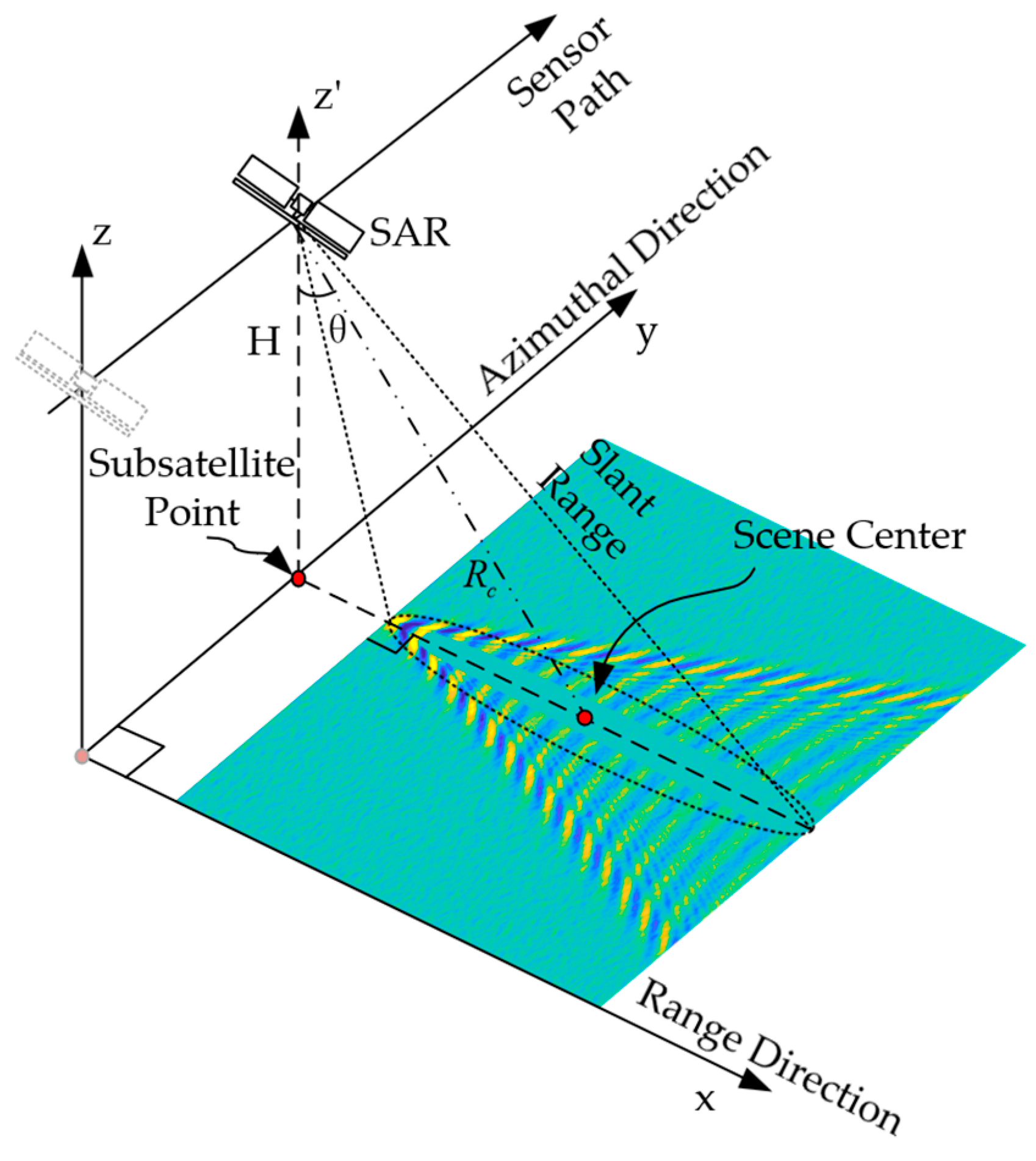
In Figure 1, the geometric relationship between SAR and the ocean ship wake scene is illustrated, and a zero squint angle and a side-looking SAR system are employed. The SAR platform travels in the azimuthal direction, maintaining an altitude of with a moving velocity of . Our SAR system continuously transmits pulse signals along the slant range direction with the speed of light , where represents the slant range and denotes the incident angle from the SAR system to the center of the ocean ship wake scene. The ratio is represented as . The x-axis is referred to as the ground range coordinate and the y-axis is referred to as the azimuth coordinate. The z-axis is positive in the upward direction.
2.1.1. Modeling of Sea Surface Scene
The simulation of the sea surface elevation , the slope of elevation along the ground range direction , and the orbital velocities along the x-axis, y-axis, and z-axis, named , , and , can be expressed as follows using the linear filtering method, respectively [31]:
where M and N are the numbers of facets in the azimuth and ground range of the ocean scene, respectively. The coordinate values are and , where and are the SAR pixel sizes in the azimuth and ground range, respectively. is the pulse repetition frequency of the radar, and is the sampling time interval for range direction. is the azimuthal sampling time, which is also called slow time. and denote the side lengths of the simulated sea surface. and represent the spatial wavenumbers of sea waves along the ground range and azimuth directions, respectively. is the angular frequency with . is the gravitational acceleration. Due to only the influence of wind-generated waves on ship wake patterns being considered in this work, we use , the Elfouhaily wave spectrum [32], to generate wind waves. The expression of in (1–5), which denotes the Fourier coefficient of the rough sea surface, can be found in [31] p. 6.
2.1.2. Modeling of Kelvin Wake
The ship wake patterns exhibit significant variability and can primarily be categorized into four distinct types: the Kelvin wake, the turbulent wake, wake generated by internal waves, and narrow-V wake [33]. In our ship wake study, the Kelvin wake and the centerline turbulent wake are simulated. The wake region where surface foam and subsurface bubbles are generated [8], leading to a significantly large NRCS [34], is not considered. The Kelvin wake, originally postulated by Lord Kelvin in 1887 [35], refers to a phenomenon associated with moving vessels in water and falls under the category of surface gravity waves. The wake pattern consists primarily of divergent waves that spread outwards from the path of vessels and transverse waves that propagate astern. Researchers have successively proposed theories related to ship wake fluid dynamics models. Michell derived the relationship between ship wake wave height and its velocity fields [15]. Wang, Eggers, and Tuck proposed various fluid dynamics numerical models related to the Kelvin wake’s wave height [16,17,18]. Then, Oumansour summarized the models in [16,17,18] and examined the detectability of simulated Kelvin wakes in airborne SAR images using both X-band and L-band frequencies [36]. We use the elevation model of Oumansour in [36] to generate the elevation of the Kelvin wake.
Assuming in a two-dimensional Cartesian coordinate system, the moving vessel travels along the negative x-axis, perpendicular to the y-axis, then the generated Kelvin wake wave height can be represented as
For a Wigley parabolic hull, assuming that the bow of the ship is at , the stern is at with a ship length of , and the submersion depth of the ship’s hull is . The angle between the ship navigation direction and direction of the Kelvin wake wave propagation is , the ship width is , and the ship speed is .
The elevation of the Kelvin wake can be written as follows [36]:
where is the viscosity coefficient. If the superposition effect of the bow and stern wakes is considered, then is set to 1. Conversely, if the superposition effect of the bow and stern wakes is not considered, is set to 0. In our article, is set to 0 in the subsequent simulation models.
The fluid mechanics relationship between the fluid velocity potential and the elevation of the Kelvin wake in [15] is expressed as
The x and y components of the wake’s velocity field are obtained by calculating partial derivatives with respect to x and y, respectively. Then, by taking the derivative of the wake wave height with respect to time, we obtain the velocity of the wake along the z-axis. The orbital velocity components along the x-axis, y-axis, and z-axis are represented as follows, respectively:
The Kelvin wake wavelength can be expressed as
2.1.3. Modeling of Turbulent Wake
Disturbances caused by breaking waves, the hull’s interaction with water, and the propulsion system of a passing ship create turbulence that initially disrupts and subsequently subsides the waves immediately trailing the vessel. This phenomenon gives rise to the turbulent wake. There is solid experimental evidence showing that the damping of waves in the turbulent wake is a result of increased viscosity, decreased temperature, and changes in the surface tension and elasticity in the surface skin of the ocean [37]. At the same time, elevated bubbles carry surface-active materials from the water column to the surface, enhancing the suppression of short gravity–capillary waves. The attenuation of the short waves in the turbulent wake leads to a considerable reduction in the radar back-scattering cross section, and as a consequence, it can darken the wake in SAR images [38]. This type of wake appears in imagery as a dark line starting in the vicinity of the ship and stretching for a few kilometers behind. The turbulent wake is the most persistent wake signature seen in SAR imagery. In 180 ERS-1 C-band images, 80% of wakes were turbulent, with the lengths ranging from 2.7 to 3.3 km. The turbulent wakes are most commonly seen under moderate wind conditions (2.5 to 7.5 m /s) [39].
Our simulation of a turbulent wake model is mainly based on Milgram’s research. Milgram proposed an empirical formula for the variation of the turbulent wake width with distance based on experimental data [21]. He also provided experimental data that demonstrate the influences of the surface tension and wind on the suppression and subsequent regrowth of short-wave energy in the turbulent wake behind a ship [22]. In our article, the width of turbulent wake is discussed before the elevation and fluid velocity are simulated.
The width variation of the turbulent wake generated by a self-propelled ship in relation to the large distance x aft the ship was initially predicted in 1957 by Birkhoff and Zarantonello [40]. It is represented as
where determines the asymptotic relation for the expansion of the width of the turbulent wake aft a ship. In the prediction by Birkhoff and Zarantonello, is set to 5, which is in good agreement with the experimental measurements performed later by Milgram and his team [22]. However, expression (15) does not include any parameters of ships and cannot be used to invert them. So, Zilman proposed a width model that takes into account the parameters of ships [41], based on the expression (15). It can be expressed as
This model expresses the power–law relationship between the width of the turbulent wake and the distance that traveled behind the ship. The parameter is an empirical factor, which is obtained from experimental measurements, and its actual value may vary due to factors such as ship type and speed. is the beam of the ship, and is set to 5, the same as in expression (15). Following Zilman’s quote in [41], the half width of the turbulent wake approximately equals to about 2 ship beams at a distance of 4 ship lengths aft of the stern [21]; thus,
Substituting (17) into (16) gives the following expression:
After performing calculations, when , and , the width of the ship can be expressed as
In our latter simulations, the turbulent wake widths are calculated using (19). Because the turbulent wake is formed as a result of disturbing factors suppressing the waves behind the ship, in our article, the wave height of turbulent wake is simulated by applying an attenuation function to the ambient sea surface elevation. Based on the upper curve of the figure in Milgram’s article [22], p. 7015, which was made using experimental C-band turbulent wake elevation data measured by buoys of the team and extracted by us using curve extraction software, it is evident that in the turbulent wake, there is a strong suppression of short waves, followed by a gradual regrowth in wind-generated waves. For the experimental data curve of Milgram, the dependent variable is filtered wave energy, which is computed from the square of the C-band wave elevation data with the application of a 2 min moving average. The independent variable is the wake age that is expressed by , where denotes the distance behind the ship.
Unfortunately, we are unable to obtain the actual data of the experimental data curve of Milgram and there are no data recorded on the experimental data curve before the wake age of 3.2 min due to the measurement method used by Milgram in [22]. Additionally, we apply the attenuation and regrowth states of the experimental C-band waves of Milgram to all bands in our simulation. The extracted curve is shown in blue in Figure 2. We employ the curve to develop a fitted attenuation function to illustrate the approximate numerical relationship between suppression as well as the restoration of waves and the wake age, aiming to simulate the attenuation and subsequent recovery of wave patterns of the turbulent wake in comparison to the wind waves outside the wake. For the extracted blue curve, as Figure 2 shows, we quote Milgram’s description about the original experimental data curve in [22] and rewrite it as follows: at the earliest measurement time, corresponding to a wake age of 3.2 min, the energy of the C-band waves had attenuated by approximately 3 dB compared to ambient sea wave energy. In the rest measurement time, the waves recover slowly toward ambient levels. In Figure 2, the red curve corresponds to the attenuation function fitted from the extracted blue curve and the horizontal axis represents the wake age with the vertical axis representing filtered wave energy on a logarithmic scale. The fitted function can be expressed as
where represents filtered wave energy on a logarithmic scale, and is the wake age in minutes.
After converting the logarithmic coordinate of filtered wave energy to linear coordinate and changing the independent variable unit from to , (20) can be written as
The value of the rearward velocity field is set to [42]. The lateral velocity field produced by the turbulent wake can be described using the Swanson model [29] as follows:
where is the distance between the two vortex centers of ship, is the depth of the vortex center, and is the dynamic current circulation given by (23):
where , is the form factor of the ship hull, and the initial circulation is
with the ship hull drag given as 0.05. In order to make continuous, we corrected the coefficient of 15 in (24) to 15.85.
In our model, we consider the temporal changes in the wake due to the movement of the ship within the scene. The elevation of the ocean ship wakes is the superposition of time-varying elevations of wind waves and ship wakes, which applies to all models, including the surface slopes model and orbital velocity fields model. Figure 3 shows the simulation results of the elevation, radial velocity, and azimuthal velocity fields of the ocean ship wakes at a certain moment, with the parameters of the ship and sea state shown in Table 1. The Kelvin wake occurs at half of the ship’s length, while the turbulent wake starts at the stern of the ship. U10 represents the wind speed at 10 m above sea level. The relative radar looking direction is identified as the angle between the radar looking direction and ship heading [43,44], while the relative wind direction is set as the angle between the wind direction and ship heading [43].
2.2. Modeling of Electromagnetic Scattering
According to the two-scale theory, the sea surface is composed of the superposition of large-scale and small-scale waves. Waves with wavelengths comparable to the length of the incident electromagnetic waves are classified as small-scale waves, while waves with wavelengths greater than the incident electromagnetic waves fall into the category of large-scale waves. The raw data strength of synthetic aperture radar system operating at moderate center incidence angles are dominated by the scattering fields from small-scale Bragg resonance waves. Large-scale waves can only be indirectly imaged by modulating the small-scale waves, given that they are beyond the radar’s direct sensitivity range.
Large-scale waves exert not only tilt modulation on small-scale waves, altering the local incident angle at different locations within the radar-to-sea scenario, but they also induce an uneven distribution of roughness in the small-scale wave field due to the motion of large-scale waves, which is referred to as hydrodynamic modulation [30]. Taking both tilt and hydrodynamic modulation effects into account, the normalized radar cross section (NRCS) of the ocean ship wake surface can be expressed as
where denotes the local incidence angle. is the ratio of group velocity to phase velocity, which is set to 0.5 here [45], as the ship wake is primarily composed of gravity waves. The relaxation rate is written as , with denoting the friction velocity and , followed by and [46]. denotes the hydrodynamic modulation transfer function (HMTF) of ocean waves, where for wind speeds ≥7 m/s, and for wind speeds <7 m/s [30]. is the ship wake velocity along the ground range direction, and its flow field gradient reflects the hydrodynamic modulation of the ship wake [26].
Considering the accuracy and computational efficiency when calculating the NRCS, we use the GMF. So, the variable in Equation (25) can be written as
which denotes the normalized radar cross section evaluated using the GMF for the C-band as CMOD5 [47,48], the X-band as XMOD2 [49], and the Ku-band as KuMOD [50], as utilized in this article. is the azimuth angle of the wind direction; pp stands for the polarization mode.
2.3. SAR Image Simulation
In order to better understand the SAR imaging mechanisms of ocean ship wakes, we study the SAR image simulation of dynamic ocean scene based on modulation theories at the echo signal level in this section. The simulation process includes the reconstruction of the ocean scene and backscattering coefficients, the generation of the raw signal, and SAR imaging algorithm. The ocean scene and electromagnetic scattering modeling have been implemented above. In this section, the SAR raw data are simulated, and RDA is used to process the echoes to obtain the SAR image of ocean ship wakes. Franceschetti proposed a method for simulating the SAR raw data of ocean scenes [51]. Liu and He presented a simulation for generating ocean SAR raw data by considering the VB effect on SAR images [52]. Li proposed a numerical simulation method of SAR imaging for time-varying sea surfaces based on raw data [30]. These three methods form the basic theory of ship wake SAR image simulation. There are two problems that need to be solved in generating SAR raw data. The first problem is that the VB effect needs to be considered, and the second problem is determining how to efficiently reflect the effect of speckle noise in the echoes.
The VB effect is a consequence of the inherent SAR imaging mechanism. We incorporate this effect into the SAR imaging process by considering the orbital velocity of the sea and ship waves. This velocity results from the orbital motion of large-scale waves, causing a variation in the relative radial velocity between the radar and sea surface. The variation leads to an additional Doppler frequency shift in the raw data, causing a change in its phase. Ultimately, this results in azimuthal displacement and blurring in SAR images, inducing distortion and reducing their resolution and clarity.
Radial velocity is the component of wave velocity along the SAR beam direction. The radial velocity can be expressed as
where denotes the ocean ground range velocity and denotes the vertical velocity of ocean ship wakes. The radial velocity of the scattering element would conduct displacement along the azimuthal direction on SAR images [53]. The displacement can be expressed by , and is the mean radial velocity during the SAR integral time.
For a time-varying ocean ship wake scenario, it is necessary to incorporate the instantaneous velocities of various scattering elements at different slow time instances into the raw data model to enhance the authenticity of the simulation results. The change in velocity over time can demonstrate the acceleration of the wake. Due to the wake motion causing changes in the slant range from the radar to the ocean surface, we introduce the velocity of large-scale waves into the slant range formula.
In a time-varying scenario, the slant range from each spatial unit to the radar is represented as
where is the time-varying closest slant range from the radar to various spatial points on the ocean surface, and denotes the ocean azimuthal velocity. Changes in this slant range formula alter the phase of the raw data, subsequently affecting the Doppler frequency and ultimately influencing the dynamic sea surface SAR image.
The time-varying ocean ship wake SAR raw data can be expressed as follows:
where is the instantaneous slant range from the SAR to the ocean surface, and it is shown in (28). denotes the fast time variable of the SAR raw data, and is the Doppler centroid time. is an approximately rectangular window as the range signal envelope. is the radar carrier frequency, is the range frequency modulation (FM) rate, and is the chirp pulse duration time with the SAR integral time . When the image process simulation does not need to consider the VB effect, the velocity and in (28) are set to 0 to illustrate that there is no orbital velocity of facets in the ocean ship wake scene. The ideal results are used for comparison with the results that consider the VB effect. Obviously, to simulate more real SAR image results, the VB effect is supposed to be considered by add and in (28).
Speckle noise is indeed present in the SAR image due to the coherent superposition of the echoes in a resolution cell. According to the statistical characteristics of speckle noise, the scattering field satisfies a complex circular Gaussian distribution with a mean of 0, and a standard deviation of the normalized backscattering coefficient can be expressed as
where and are two independent Gaussian random numbers.
3. Discussion of Simulation Images
Based on a SAR platform with fixed parameters such as platform altitude, velocity, and imaging resolution, the SAR imaging simulation of ocean ship wakes are affected by a series of other parameters, such as the electromagnetic wave bands and polarization modes emitted by SAR, the center incidence angles of the SAR platform, U10, ship speeds and relative wind directions, and relative radar looking directions. In this section, the impacts of the above parameters on the SAR simulation images are discussed. The parameters of the SAR platform, the ship, and the sea state are listed in Table 2.
Figure 4 shows the variation of the NRCS with the incidence angle for different frequency bands and polarization modes, calculated using the GMF with U10 = 5 m/s, 7.5 m/s, and 10 m/s, respectively. The Ku-band NRCS is calculated using KuMOD, the X-band NRCS is obtained from XMOD2, and the C-band NRCS is computed using CMOD5. As the wind speeds increase from Figure 4a–c, the NRCS values enhance accordingly. In detail, it is obvious in Figure 4a that within the range of the incidence angle of 30 to 50 degrees, both the HH polarization and VV polarization of the X-band have higher NRCS values than those of the C-band, with the HH polarization of the C-band having the lowest value in this interval. When the incidence angle is between 40 and 50 degrees, both the HH polarization and VV polarization of the X-band have higher NRCS values than those of the Ku-band, with the VV polarization of the X-band having the highest value in this interval. Most importantly, when the incidence angle ranges from 25 to 50 degrees, all VV polarization NRCS values for each frequency band are higher than their corresponding HH polarization NRCS values.
In Figure 5, the numerical simulation results of SAR ocean ship wakes under different radar electromagnetic wavebands and polarization modes are presented. The U10 is 5 m/s, the center incidence angle is 40°, the ship speed is 10 m/s, and the relative radar looking direction is 180°. It can be seen that twelve images are arranged in two columns, with six rows in each column. During the simulation process of six images of the left column, the VB effect caused by the motion velocity of facets in the scene is considered, while conversely, those in the right column do not consider this effect. The images in different rows display the SAR simulation results under different wave bands, including the C-band VV polarization in Figure 5a,b, the C-band HH polarization in Figure 5c,d, the X-band VV polarization in Figure 5e,f, the X-band HH polarization in Figure 5g,h, the Ku-band VV polarization in Figure 5i,j, and the Ku-band HH polarization in Figure 5k,l.
In Figure 4a, it can be observed that under an incidence angle of 40 degrees and a wind speed of 5 m/s, the NRCS exhibits a sequential rise in the VV polarization in the C, Ku, and X-bands, and the same applies to the HH polarization. Additionally, not only is the VV polarization NRCS greater than the HH polarization NRCS for the corresponding bands, but the lowest C band NRCS in the VV polarization is also higher than the highest X band NRCS in HH polarization. According to the process of SAR imaging, the higher the NRCS in the scene, the stronger the simulated SAR image intensity value. Thus, in Figure 5, it is obvious that the SAR image intensity is the lowest in the C band HH polarization in Figure 5c,d and the highest in the X band VV polarization in Figure 5e,f.
It can be observed that when the VB effect is not considered, in all three electromagnetic wavebands, the details of the Kelvin wake transverse waves and divergent waves are clearly visible, as Figure 5b,d,f,h,j,l show. The Kelvin wake regions that have higher wave elevations exhibit brighter stripes compared to the dark stripes where the wave elevations are lower. In the VV polarization SAR images in Figure 5b,f,j, the turbulent wake features near the stern of the ship are seen to be very dark, and with an increasing distance behind the ship, the texture of the turbulent wake gradually becomes brighter as the elevations of the suppressed small-scale waves within the wake grow towards those of the ambient wind waves. Furthermore, the small-scale waves in the turbulent wake region in the HH polarization SAR images of the waves in Figure 5d,h,l exhibit less texture clarity compared to the corresponding VV polarization SAR images of the three bands in Figure 5b,f,j, meaning the image intensity and NRCS of the former are lower than those of the latter, which corroborates the quantitative analysis mentioned earlier.
According to the aforementioned theory, the VB effect causes a noticeable displacement and a blurring of facets in the ocean ship wake scene, and under other equal conditions, the greater the radial velocity of the facet, the larger the azimuthal offset, which is visually evident in Figure 5a,c,e,g,i,k, respectively. In detail, comparing Figure 5a,b, it can be observed that, at range distances of 0–20 m and 60–80 m, the bright Kelvin waves there that have higher radial velocities towards the radar platform experience more significant offsets due to the VB effect compared to the other bright Kelvin wake regions. In addition, the dark Kelvin waves that have radial velocities directed away from the radar cause an offset in the opposite direction to that of bright Kelvin waves. This leads to more prominent peaks and troughs in the transverse waves of the Kelvin wake in Figure 5a, also resulting in a bright line formed by the connected wave peaks in the starboard Kelvin arm, and a dark line formed by the connected wave troughs in the port Kelvin arm. Due to the relatively low orbital velocity of facets in the turbulent wake compared to that of the Kelvin wake and wind waves, their azimuthal offset is not significant. At the same time, the ambient wind wave patterns in Figure 5a are noticeably different from those in Figure 5b, because the radiative convergence and divergence are more pronounced for wind wave peaks and troughs in Figure 5a. Additionally, due to constant SAR platform parameters and the fact that the velocities of facets in the scene remain unchanged with variations in the radar frequency bands and polarization modes, the displacement and blurring induced by the VB effect for each facet also remain unaffected by such changes.
In Figure 6, the simulation SAR images of ocean ship wakes under different wind speeds are presented. The center incidence angle is 40°, the ship speed is 10 m/s, and the relative radar looking direction is 180°. The imaging waveband is the C-band with VV polarization. The three images of the left column in Figure 6 are the results that consider the VB effect, while conversely, those in the right column are the results that do not consider this effect. The images in different rows display the SAR simulation results under different wind speeds, including U10 of 5 m/s, 7.5 m/s, and 10 m/s, respectively. From Figure 4, it follows that the stronger the wind speed, the higher the NRCS under the same conditions. So, the results with a U10 of 10 m/s in Figure 6e,f have the strongest SAR image intensities due to them having the highest NRCS values, while those with a U10 of 5 m/s in Figure 6a,b have the weakest image intensities.
When the VB effect is not considered, with an increase in the wind speed, the visualization of the ship wake’s signature in the SAR image becomes more difficult in Figure 6b,d,f. As can be observed, the scale of ambient wind waves progressively increases from Figure 6b–f. In the ship wake region, the results with a U10 of 7.5 m/s in Figure 6d and with a U10 of 10 m/s in Figure 6f only display divergent waves and turbulent wake. It is noteworthy that the divergent waves in Figure 6f appear blurrier than those in Figure 6d. This is due to the influence of an increased wave height, which disturbs the textures of Kelvin transverse waves and divergent waves, as seen in the SAR simulation results of the ocean Kelvin wake shown in [25]. In Figure 6b,d,f, the turbulent wakes progressively become brighter because, as the wind speed increases, the small-scale waves in the turbulent wake region regenerate more rapidly.
Considering the VB effect, when the U10 is 5 m/s, given the existing ship speed, the additional energy input in the scene is minimal, and the velocity of the facets is relatively low. Compared with Figure 6c,e, the textures of the ship wakes in Figure 6a have only been weakly smeared by the VB effect due to the orbital velocity of the facets. With an increasing wind speed, the energy input increases, resulting in an enhancement in the velocity of the facets in the scene. Together with their different motion directions, this leads to an increase in the offset of the facets both in the positive and negative azimuthal directions, resulting in a more pronounced streaking effect, as seen in Figure 6c,e. Due to this phenomenon, the texture of the Kelvin wake is disrupted and blurred, while the texture of the turbulence wake is masked.
In Figure 7, the simulation SAR images of ocean ship wakes under different center incidence angles are shown. The wind speed is 5 m/s, the ship speed is 10 m/s, and the relative radar looking direction is 180°. The imaging waveband is the C-band with VV polarization. The two images of the left column in Figure 7 are the results that consider the VB effect, while those in the right column do not consider this effect. The images in different rows display SAR simulation results under center incidence angles of 30° and 40°, respectively.
Figure 4 emphasizes that when the other conditions are the same, when the radar center incidence angle is within a certain range, the lower the angle, the higher the NRCS. So, in Figure 7, the results with a center incidence angle of 30° in Figure 7a,b have stronger SAR image intensities than those with a center incidence angle of 40° in Figure 7c,d. In Figure 7b, the textures of the ambient wind waves, Kelvin wake, and turbulent wake are more visible than those in Figure 7d. Comparing the turbulent wake region of the two images, the small-scale waves suppressed behind the ship, represented as black regions in the image, show a more noticeable contrast when compared to the gradually brightening regions, where they progressively regrow with increasing distance behind the ship in Figure 7b. After considering the VB effect on the offset of facets, in Figure 7a, the peaks and troughs of the ambient wind waves and Kelvin wake are more obvious than those in Figure 7c.
The SAR simulation imaging results of ocean ship wakes with different ship speeds are presented in Figure 8. The wind speed is 5 m/s, and the relative radar looking direction is 180°. The imaging waveband is the C-band with VV polarization, and the center incidence angle is 40°. The three images of the left column in Figure 8 are the results that consider the VB effect, while those in the right column do not consider this effect. The images in different rows display SAR simulation results under ship speeds of 7.5 m/s, 10 m/s, and 12.5 m/s, respectively. At a fixed wind speed and center incidence angle, there is almost no difference in the image intensity in Figure 8a–f.
When the VB effect is not considered in Figure 8b,d,f, as the ship speed enhances, both the transverse wave and divergent wave lengths of the Kelvin wake grow larger, resulting in wider spacing between the bright and dark stripes in the Kelvin wake region in the SAR images, which also verifies Equation (14). The texture of the turbulent wake in Figure 8b,d,f does not vary with the ship speed because the regrowth of small-scale waves in the turbulent wake region is unrelated to it. By comparing the texture of the ambient wind wave region and ship wake region after considering the VB effect in Figure 8a,c,e, we can observe that while the constant wind speed does not lead to a significant change in the displacement and blurring of the ambient wind waves, the displacements of facets in the ship wake region intensify with an increasing ship speed. This is because the wake wave velocity at a fixed position behind the ship enhances with the ship speed. In detail, at the range distances of 0–20 m and 60–80 m, the bright Kelvin waves in Figure 8e exhibit the most significant displacement compared to Figure 8a,c, which have the highest radial velocities in this region among the three images. By the same token, in Figure 8e, the displacement of facets at any wave peak or trough in the Kelvin wake is more pronounced than in Figure 8c, and it is also more serious than in Figure 8a. Even the velocity of the turbulent wake is influenced by the ship speed, as Equations (22)–(24) show, due to the value being very minimal compared to the velocity of the Kelvin wake and ambient wind waves; the texture of the turbulent wake in Figure 8a,c,e do not have noticeable displacement and blur.
The SAR simulation results of ocean ship wakes with different relative radar looking directions are presented in Figure 9. The relative radar looking direction is identified as the angle between the radar looking direction and ship heading [43,44], while the relative wind direction is set as the angle between the wind direction and ship heading [43]. The wind speed is 5 m/s, the center incidence angle is 40°, and the ship speed is 10 m/s. The imaging waveband is the C band with VV polarization. The three images of the left column in Figure 9 are the results that consider the VB effect, while those in the right column do not consider the effect. Our parameters are set as follows to discuss the imaging results under different relative radar looking directions in Figure 9. In the simulation results of the first, second, and third rows in Figure 9, the relative radar looking directions are 180°, 135°, and 90°, respectively. The relative wind direction is fixed as 180.
When the VB effect is not considered, both the port and starboard Kelvin divergent waves appear to be clear bright with dark stripes in Figure 9b because they propagate along the radar looking direction. In this case, both the tilt and hydrodynamic modulation terms make significant contributions to the relative NRCS of the two sides of divergent waves. But in Figure 9d, when the port Kelvin divergent waves are more perpendicular to the radar looking direction than the starboard Kelvin divergent waves, the former are at a lower visibility than the latter due to the tilt and hydrodynamic modulation of the port waves making extremely weak contributions to the NRCS. In Figure 9f, the textures of the port Kelvin divergent waves are less visible than those of the starboard ones. The reason for this phenomenon is that the contributions of tilt and hydrodynamic modulation terms on the NRCS of the port one calculated by Equation (25) are partly offset, while those of the starboard one all make relative effective contributions. In terms of the Kelvin transverse waves, the causes of their visible textures in Figure 9b, their relatively darker textures in Figure 9d, and their completely invisible textures in Figure 9f are also related to the impacts of tilt and hydrodynamic modulation on the NRCS. Due to the already low NRCS in the turbulence wake region, it is hardly affected by the variation in the effects of tilt and hydrodynamic modulation with changes in the relative radar looking directions.
After considering the VB effect, in the ambient ocean wave regions in Figure 9a,c,e, the peaks and troughs of the wind waves become more pronounced due to the displacement of facets along the azimuthal direction when compared to those in Figure 9b,d,f, respectively. In Figure 9c, the facets in the region of the starboard Kelvin divergent waves exhibit distinct displacement. The textures of the starboard Kelvin transverse waves are blurrier than those of the port side. This is due to a more pronounced displacement of facets in this region, leading to a more severe disturbance of the texture. This occurs because, for two facets symmetrically positioned with respect to the centerline of the turbulent wake extending directly behind the ship in the transverse wave region, the starboard facet has a higher radial velocity as a result of the transverse waves’ propagation directions. The facets in the port Kelvin transverse wave region exhibit slight displacement. In Figure 9e, due to the azimuthal displacement of the divergent waves, the texture of the Kelvin wake is almost completely blurred, while the peaks and troughs of the starboard divergent waves with the maximum wavelength are quite prominent, with those on the port side being slightly visible. The former discussion of our simulation results in this part is in good agreement with the analysis of the detectability of Kelvin arms under different relative radar looking directions in the work by Henning [43].
The SAR simulation results of ocean ship wakes with different relative wind directions are presented in Figure 10. The wind speed is 5 m/s, the center incidence angle is 40°, and the ship speed is 10 m/s. The imaging waveband is the C band with VV polarization. The relative radar looking direction is fixed as 180°. The two images of the left column in Figure 10 are the results that consider the VB effect, while those in the right column do not consider the effect. Our parameters are set as follows to discuss the imaging results under different relative wind directions: in the simulation results of the first and second rows in Figure 10, the relative wind directions are set as 180 and 135°, respectively.
When the VB effect is not considered, in Figure 10b,d, both the port and starboard Kelvin divergent waves can be clearly seen. This is mainly because the tilt and hydrodynamic modulation terms make significant contributions to the relative NRCS of the two sides of divergent waves, as the relative radar looking direction is fixed [43]. Comparing the textures of the Kelvin wake regions in Figure 10b,d, the NRCS is not significantly affected by the changing relative wind direction. However, the result with a 180° relative wind direction in Figure 10b has a stronger SAR image intensity than the result in Figure 10d with a 135° relative wind direction, because relative wind directions have influences on the NRCS in SAR images, as discussed by Hennings [43]. In this case, the turbulent wake in Figure 10d is more visible than in Figure 10b. When the VB effect is considered, in Figure 10a,c, the displacement of facets with different radial velocities along the azimuthal direction leads to pronounced peaks and troughs in the Kelvin wake region. In the ambient ocean wave regions in Figure 10a,c, the peaks and troughs of the wind waves also become more visible than those in Figure 10b,d. Also, the result with a 180° relative wind direction in Figure 10a has a stronger SAR image intensity than in Figure 10c with a 135° relative wind direction.
4. Conclusions
In conclusion, our research introduced a numerical simulation method for acquiring SAR images of time-varying ocean ship wakes under various radar, ship, and sea surface conditions. First, we employed the linear filtering method, classic fluid dynamics models, and attenuation function method to simulate the time-varying elevation and velocity fields of the wind waves, Kelvin wakes, and turbulence wakes, respectively. Then, within our established SAR imaging platform, we obtained the raw data of ocean ship wakes by calculating backscattering fields using geophysical model functions (GMFs) and accounting for the changing slant range. Furthermore, we applied the Range-Doppler algorithm (RDA) for pulse compression and range cell migration correction (RCMC) to generate SAR images based on the raw data. Our simulation took into consideration the velocity bunching (VB) effect due to large-scale waves and the influence of speckle noise.
A comparison was made between SAR images considering the VB effect and those not considering the VB effect. Throughout our research, we demonstrated that radar electromagnetic wavebands, polarization modes, wind speeds, ship speeds, relative radar looking directions, and relative wind direction all have distinct impacts on the SAR imaging results of ocean ship wakes. In discussing the electromagnetic wavebands and polarization modes, the details of the ship wakes are all clearly visible, but the SAR image intensity varies due to differences in the NRCS. As the wind speed increases, the SAR image intensity becomes stronger, but due to the more serious VB effect, it causes the texture of the wake to be blurred by the offset of the facets in the scene. At moderate radar center incidence angles, a reduction in the center incidence angle leads to an increase in the SAR image intensity, resulting in a clearer wake texture. Additionally, the wavelength of the Kelvin wake becomes larger as the ship speed increases. The increasing ship speed also causes a higher ship wake velocity, leading to a more significant offset of the facets in the Kelvin wake region caused by the VB effect. Due to the velocity of turbulent wake being very minimal compared to the velocity of the Kelvin wake and ambient wind waves, the texture of the turbulent wake does not have noticeable displacement and blur. When the relative radar direction changes, the morphology of the wake in SAR images undergoes alterations. Specifically, the visibility of the arms of the Kelvin wake varies with the contributions that the tilt and hydrodynamic modulation of the arms make to its NRCS. Due to the already low NRCS in the turbulence wake region, it is hardly affected by the variation in the effects of the tilt and hydrodynamic modulation with changes in the relative radar looking directions. The SAR image intensity varies with the relative wind directions, while the textures of the Kelvin wakes do not significantly change when the wind speed is 5 m/s. In summary, our work can provide SAR images with different radar and sea surface conditions for various ship parameters, enabling more comprehensive investigations on ship wake simulation. In the future, we will explore SAR imaging simulations of a broader range of ship wakes, including internal wave wakes and narrow-V wakes. In the next step, we will focus on finding suitable simulation models to simulate the elevation fields and their velocity fields. Because under the two-scale theory of ocean waves we mentioned before, these fields play key roles in the tilt and hydrodynamic modulation. The orbital velocity also influences the displacement of the facet on the SAR image when the VB effect is considered. We will also investigate imaging outcomes under various conditions, such as the influence of swell waves on ocean ship wake SAR imaging.
Author Contributions
Conceptualization: S.W. and Y.W.; methodology: S.W., Y.W. and Q.L.; validation: Y.W. and Y.Z.; software: S.W., Y.W., Q.L., Y.B. and H.Z.; formal analysis: S.W. and Y.W.; investigation: S.W., Y.W., Q.L. and Y.Z.; writing—original draft preparation: S.W.; writing—review and editing, S.W., Y.W., Q.L. and Y.Z.; funding acquisition: Y.W. and H.Z. All authors have read and agreed to the published version of the manuscript.
Funding
This research was funded by the National Natural Science Foundation of China under Grant Nos. 41976167, 42376176, 52101393, and the Laoshan Laboratory science and technology innovation projects under Grant LSKJ202201302. It was also supported in part by the Natural Science Foundation of Shandong Province under Grant No. ZR2021QD001.
Data Availability Statement
No new data were created or analyzed in this study. Data sharing is not applicable to this article.
Conflicts of Interest
The authors declare no conflict of interest.
References
- Cumming, I.G.; Wong, F.H. Digital Processing of Synthetic Aperture Radar Data: Algorithms and Implementation. Artech House 2005, 1, 108–110. [Google Scholar]
- Franceschetti, G.; Iodice, A.; Riccio, D.; Ruello, G.; Siviero, R. SAR Raw Signal Simulation of Oil Slicks in Ocean Environments. Trans. Geosci. Remote Sens. 2002, 40, 1935–1949. [Google Scholar] [CrossRef]
- Li, X.; Pichel, W.; Yang, X. Spaceborne sar Imaging of Coastal Ocean Phenomena. In Proceedings of the 2010 IEEE International Geoscience and Remote Sensing Symposium, Honolulu, HI, USA, 25–30 July 2010. [Google Scholar]
- Eldhuset, K. An automatic ship and ship wake detection system for spaceborne SAR images in coastal regions. IEEE Trans. Geosci. Remote Sens. 1996, 34, 1010–1019. [Google Scholar] [CrossRef]
- Ai, J.; Yang, X.; Song, J.; Dong, Z.; Jia, L.; Zhou, F. An Adaptively Truncated Clutter-Statistics-Based Two-Parameter CFAR Detector in SAR Imagery. IEEE J. Ocean. Eng. 2017, 43, 267–279. [Google Scholar] [CrossRef]
- Zhai, L.; Li, Y.; Su, Y. Inshore Ship Detection via Saliency and Context Information in High-Resolution SAR Images. IEEE Geosci. Remote Sens. Lett. 2016, 13, 1870–1874. [Google Scholar] [CrossRef]
- Lin, H.; Chen, H.; Jin, K.; Zeng, L.; Yang, J. Ship Detection with Superpixel-Level Fisher Vector in High-Resolution SAR Images. IEEE Geosci. Remote Sens. Lett. 2019, 17, 247–251. [Google Scholar] [CrossRef]
- Reed, A.M.; Milgram, J.H. SHIP WAKES AND THEIR RADAR IMAGES. Annu. Rev. Fluid Mech. 2002, 34, 469–502. [Google Scholar] [CrossRef]
- Gasparovic, R. Observation of ship wakes from space. In Proceedings of the Space Programs and Technologies Conference, Huntsville, AL, USA, 26–28 September 1995. [Google Scholar]
- Fan, K.; Zhang, H.; Liang, J.; Chen, P.; Xu, B.; Zhang, M. Analysis of ship wake features and extraction of ship motion parameters from SAR images in the Yellow Sea. Front. Earth Sci. 2019, 13, 588–595. [Google Scholar] [CrossRef]
- Wang, H.; Nie, D.; Zuo, Y.; Tang, L.; Zhang, M. Nonlinear Ship Wake Detection in SAR Images Based on Electromagnetic Scattering Model and YOLOv5. Remote Sens. 2022, 14, 5788. [Google Scholar] [CrossRef]
- Karakus, O.; Rizaev, I.; Achim, A. Ship Wake Detection in SAR Images via Sparse Regularization. IEEE Trans. Geosci. Remote Sens. 2019, 58, 1665–1677. [Google Scholar] [CrossRef]
- Tings, B.; Pleskachevsky, A.; Wiehle, S. Comparison of detectability of ship wake components between C-Band and X-Band synthetic aperture radar sensors operating under different slant ranges. ISPRS J. Photogramm. Remote Sens. 2023, 196, 306–324. [Google Scholar] [CrossRef]
- Kang, K.-M.; Kim, D.-J. Ship Velocity Estimation from Ship Wakes Detected Using Convolutional Neural Networks. IEEE J. Sel. Top. Appl. Earth Obs. Remote Sens. 2019, 12, 4379–4388. [Google Scholar] [CrossRef]
- Michell, J.H. XI. The wave-resistance of a ship. Lond. Edinb. Dublin Philos. Mag. J. Sci. 1898, 45, 106–123. [Google Scholar] [CrossRef]
- Wang, H. Spectral comparisons of ocean waves and Kelvin ship waves. In Proceedings of the Seventh Offshore Mechanics and Arctic Engineering Symposium, New York, NY, USA, 7 February 1988; Volume 2, pp. 253–261. [Google Scholar]
- Eggers, K.W.H. An Assessment of Some Experimental Methods for Determining the Wave-making Characteristics of a Ship Form. Trans Sname 1967, 75, 112–157. [Google Scholar]
- Tuck, E.O.; Collins, J.I.; Wells, W.H. On Ship Wave Patterns and Their Spectra. J. Ship Res. 1971, 15, 11–21. [Google Scholar] [CrossRef]
- Fujimura, A.; Soloviev, A.; Kudryavtsev, V. Numerical Simulation of the Wind-Stress Effect on SAR Imagery of Far Wakes of Ships. IEEE Geosci. Remote Sens. Lett. 2010, 7, 646–649. [Google Scholar] [CrossRef]
- Fujimura, A.; Soloviev, A. Approaches to Validation of CFD Models for Far Ship Wake. AGU Fall Meet. Abstr. 2008, 1, 1260. [Google Scholar]
- Milgram, J.H.; Skop, R.A.; Peltzer, R.D.; Griffin, O.M. Modeling short sea wave energy distributions in the far wakes of ships. J. Geophys. Res. Ocean. 1993, 98, 7115–7124. [Google Scholar] [CrossRef]
- Milgram, J.H.; Peltzer, R.D.; Griffin, O.M. Suppression of short sea waves in ship wakes: Measurements and observations. J. Geophys. Res. Oceans 1993, 98, 7103–7114. [Google Scholar] [CrossRef]
- Zilman, G.; Zapolski, A.; Marom, M. On Detectability of a Ship’s Kelvin Wake in Simulated SAR Images of Rough Sea Surface. IEEE Trans. Geosci. Remote Sens. 2014, 53, 609–619. [Google Scholar] [CrossRef]
- Shemer, L.; Kagan, L.; Zilman, G. Simulation of ship wake image by an along track interferometric SAR. In Proceedings of the 1995 International Geoscience and Remote Sensing Symposium, IGARSS’95. Quantitative Remote Sensing for Science and Applications, Firenze, Italy, 10–14 July 1995. [Google Scholar]
- Rizaev, I.G.; Karakuş, O.; Hogan, S.J.; Achim, A. Modeling and SAR imaging of the sea surface: A review of the state-of-the-art with simulations. ISPRS J. Photogramm. Remote Sens. 2022, 187, 120–140. [Google Scholar] [CrossRef]
- Wang, A. The Simulation Study of Ocean Ship Wakes lmaging by SAR. Ph.D. Thesis, University of Chinese Academy of Sciences, Beijing, China, 2003. [Google Scholar]
- Wang, J.-K.; Zhang, M.; Cai, Z.-H.; Chen, J.-L. SAR imaging simulation of ship-generated internal wave wake in stratified ocean. J. Electromagn. Waves Appl. 2017, 31, 1101–1114. [Google Scholar] [CrossRef]
- Zhang, Y.; Xiao, T.; Guo, L.; Li, H. Effect of Wind Speed on Internal Wave Imaging of Multi-polarimetric Spaceborne SAR. In Proceedings of the 2020 IEEE Radar Conference (RadarConf20), Florence, Italy, 21–25 September 2020. [Google Scholar]
- Skoelv, A.; Wahl, T.; Eriksen, S. Simulation of SAR Imaging of Ship Wakes. In Proceedings of the International Geoscience and Remote Sensing Symposium, ‘Remote Sensing: Moving Toward the 21st Century’, Edinburgh, UK, 12–16 September 1988. [Google Scholar]
- Li, Q.; Zhang, Y.; Wang, Y.; Bai, Y.; Zhang, Y.; Li, X. Numerical Simulation of SAR Image for Sea Surface. Remote Sens. 2022, 14, 439. [Google Scholar] [CrossRef]
- Guo, L. Basic Theory and Method of Random Rough Surface Scattering; Science Press: Beijing, China, 2010. [Google Scholar]
- Elfouhaily, T.; Chapron, B.; Katsaros, K.; Vandemark, D. A unified directional spectrum for long and short wind-driven waves. J. Geophys. Res. Ocean. 1997, 102, 15781–15796. [Google Scholar] [CrossRef]
- Lyden, J.D.; Hammond, R.R.; Lyzenga, D.R.; Shuchman, R.A. Synthetic aperture radar imaging of surface ship wakes. J. Geophys. Res. Atmos. 1988, 93, 12293–12303. [Google Scholar] [CrossRef]
- Donelan, M.A.; Haus, B.K.; Reul, N.; Plant, W.J.; Stiassnie, M.; Graber, H.C.; Brown, O.B.; Saltzman, E.S. On the limiting aerodynamic roughness of the ocean in very strong winds. Geophys. Res. Lett. 2004, 31. [Google Scholar] [CrossRef]
- Thomson, W. On Ship Waves. Proc. Inst. Mech. Eng. 1887, 38, 409–434. [Google Scholar] [CrossRef]
- Oumansour, K.; Wang, Y.; Saillard, J. Multifrequency SAR observation of a ship wake. Iee Proc.–Radar, Sonar Navig. 1996, 143, 275–280. [Google Scholar] [CrossRef]
- Peltzer, R.D.; Griffin, O.M.; Barger, W.R.; Kaiser, J.A.C. High-resolution measurement of surface-active film redistribution in ship wakes. J. Geophys. Res. Ocean. 1992, 97, 5231–5252. [Google Scholar] [CrossRef]
- Peltzer, R.; Garrett, W.; Smith, P. A remote sensing study of a surface ship wake. In Proceedings of the OCEANS ‘85—Ocean Engineering and the Environment, San Diego, CA, USA, 12–14 November 1985. [Google Scholar]
- McCandless, S.W.; Jackson, C.R. Synthetic Aperture Radar: Marine User’s Manual; US Department of Commerce: Washington, DC, USA, 2004.
- Birkhoff, G.; Zarantonello, E.H. Jets, Wakes and Cavities; Academic Press: New York, NY, USA, 1957. [Google Scholar]
- Zilman, G.; Zapolski, A.; Marom, M. The speed and beam of a ship from its wake’s SAR images. IEEE Trans. Geosci. Remote Sens. 2004, 42, 2335–2343. [Google Scholar] [CrossRef]
- Liu, P.; Ren, W.J.; Jin, Y.Q. SAR Image Simulation of Ship Turbulent Wake Using Semi-Empirical Energy Spectrum. In Proceedings of the 2020 IEEE International Conference on Computational Electromagnetics (ICCEM), Singapore, 24–26 August 2020. [Google Scholar]
- Hennings, I.; Romeiser, R.; Alpers, W.; Viola, A. Radar imaging of Kelvin arms of ship wakes. Int. J. Remote Sens. 1999, 20, 2519–2543. [Google Scholar] [CrossRef]
- Tings, B. Non-Linear Modeling of Detectability of Ship Wake Components in Dependency to Influencing Parameters Using Spaceborne X-Band SAR. Remote Sens. 2021, 13, 165. [Google Scholar] [CrossRef]
- Alpers, W.; Hennings, I. A theory of the imaging mechanism of underwater bottom topography by real and synthetic aperture radar. J. Geophys. Res. Ocean. 1984, 89, 10529–10546. [Google Scholar] [CrossRef]
- Romeiser, R.; Alpers, W. An improved composite surface model for the radar backscattering cross section of the ocean surface: 2. Model response to surface roughness variations and the radar imaging of underwater bottom topography. J. Geophys. Res. Ocean. 1997, 102, 25251–25267. [Google Scholar] [CrossRef]
- Hersbach, H.; Stoffelen, A.; de Haan, S. An improved C-band scatterometer ocean geophysical model function: CMOD5. J. Geophys. Res. Ocean. 2007, 112. [Google Scholar] [CrossRef]
- Zhang, B.; Perrie, W.; He, Y. Wind speed retrieval from RADARSAT-2 quad-polarization images using a new polarization ratio model. J. Geophys. Res. Ocean. 2011, 116. [Google Scholar] [CrossRef]
- Li, X.M.; Lehner, S. Algorithm for Sea Surface Wind Retrieval from TerraSAR-X and TanDEM-X Data. IEEE Trans. Geosci. Remote Sens. 2014, 52, 2928–2939. [Google Scholar] [CrossRef]
- Wentz, F.J.; Smith, D.K. A model function for the ocean-normalized radar cross section at 14 GHz derived from NSCAT observations. J. Geophys. Res. Ocean. 1999, 104, 11499–11514. [Google Scholar] [CrossRef]
- Franceschetti, G.; Migliaccio, M.; Riccio, D. On ocean SAR raw signal simulation. IEEE Trans. Geosci. Remote Sens. 1998, 36, 84–100. [Google Scholar] [CrossRef]
- Liu, B.; He, Y. SAR Raw Data Simulation for Ocean Scenes Using Inverse Omega-K Algorithm. IEEE Trans. Geosci. Remote Sens. 2016, 54, 6151–6169. [Google Scholar] [CrossRef]
- Lyzenga, D.R. Numerical Simulation of Synthetic Aperture Radar Image Spectra for Ocean Waves. IEEE Trans. Geosci. Remote Sens. 1986, GE-24, 863–872. [Google Scholar] [CrossRef]
Figure 1.
The illustration of SAR imaging platform.

Figure 2.
The experimental data of Milgram and the fitted attenuation function used to describe the wave energy of the turbulent wake. The blue line represents the data extracted directly from the figure in [22], p7015, while the red line represents the attenuation function fitted from the blue line.

Figure 3.
The simulation of elevation, radial velocity, and azimuthal velocity of ocean ship wakes. (a) The elevation field. (b) The radial velocity field. (c) The azimuthal velocity field.
Figure 3.
The simulation of elevation, radial velocity, and azimuthal velocity of ocean ship wakes. (a) The elevation field. (b) The radial velocity field. (c) The azimuthal velocity field.

Figure 4.
The NRCS values of the different GMF, polarization modes, and U10 with the incidence angle varying from 25° to 50°. (a) The NRCS values when U10 = 5 m/s. (b) The NRCS values when U10 = 7.5 m/s. (c) The NRCS values when U10 = 10 m/s.
Figure 4.
The NRCS values of the different GMF, polarization modes, and U10 with the incidence angle varying from 25° to 50°. (a) The NRCS values when U10 = 5 m/s. (b) The NRCS values when U10 = 7.5 m/s. (c) The NRCS values when U10 = 10 m/s.

Figure 5.
The SAR simulation images of ocean ship wake with the VB effect under different radar electromagnetic wavebands and polarization modes: (a) The C-band VV. (c) The C-band HH. (e) The X-band VV. (g) The X-band HH. (i) The-Ku band VV. (k) The Ku-band HH; without the VB effect under different radar electromagnetic wavebands and polarization modes: (b) The C-band VV. (d) The C-band HH. (f) The X-band VV. (h) The X-band HH. (j) The Ku-band VV. (l) The Ku-band HH.


Figure 6.
The SAR simulation images of ocean ship wakes with the VB effect under different wind speeds: (a) U10 = 5 m/s. (c) U10 = 7.5 m/s. (e) U10 = 10 m/s; without the VB effect under different wind speeds: (b) U10 = 5 m/s. (d) U10 = 7.5 m/s. (f) U10 = 10 m/s.
Figure 6.
The SAR simulation images of ocean ship wakes with the VB effect under different wind speeds: (a) U10 = 5 m/s. (c) U10 = 7.5 m/s. (e) U10 = 10 m/s; without the VB effect under different wind speeds: (b) U10 = 5 m/s. (d) U10 = 7.5 m/s. (f) U10 = 10 m/s.

Figure 7.
The SAR simulation images of ocean ship wakes with the VB effect under different incidence angles. (a) The center incidence angle is 30°. (c) The center incidence angle is 40°; without the VB effect under different center incidence angles: (b) The center incidence angle is 30°. (d) The center incidence angle is 40°.

Figure 8.
The SAR simulation images of ocean ship wakes with the VB effect under different ship speeds: (a) U = 7.5 m/s. (c) U = 10 m/s. (e) U = 12.5 m/s; without the VB effect under different ship speeds: (b) U = 7.5 m/s. (d) U = 10 m/s. (f) U = 12.5 m/s.
Figure 8.
The SAR simulation images of ocean ship wakes with the VB effect under different ship speeds: (a) U = 7.5 m/s. (c) U = 10 m/s. (e) U = 12.5 m/s; without the VB effect under different ship speeds: (b) U = 7.5 m/s. (d) U = 10 m/s. (f) U = 12.5 m/s.


Figure 9.
The SAR simulation images of ocean ship wakes with the VB effect under different relative radar looking directions: (a) direction of 180°, (c) direction of 135°, (e) direction of 90°; without the VB effect under different relative radar looking directions: (b) direction of 180°, (d) direction of 135°, (f) direction of 90°.

Figure 10.
The SAR simulation images of ocean ship wakes with the VB effect under different relative wind directions: (a) direction of 180°, (c) direction of 135°; without the VB effect under different relative wind directions: (b) direction of 180°, (d) direction of 135°.
Figure 10.
The SAR simulation images of ocean ship wakes with the VB effect under different relative wind directions: (a) direction of 180°, (c) direction of 135°; without the VB effect under different relative wind directions: (b) direction of 180°, (d) direction of 135°.


Table 1.
The parameters of the ship and sea state in Figure 3.
Table 1.
The parameters of the ship and sea state in Figure 3.
| Parameters | Values |
|---|---|
| U10 | 5 m/s |
| Relative wind direction | 180° |
| Ship length | 160 m |
| Ship beam | 32 m |
| Ship speed | 10 m/s |
| Relative radar looking direction | 180° |
Table 2.
The parameters of the SAR platform and the ocean ship wake scene in later simulations.
| Parameters | Values |
|---|---|
| Carrier frequency | 6 GHz, 10 GHz, 12 GHz |
| Pulse duration | 5 μs |
| Chirp bandwidth | 194 MHz |
| Azimuth bandwidth | 4375 Hz |
| Center incidence angle | 30°, 40° |
| Platform velocity | 7.9 km/s |
| Platform altitude | 200 km |
| Azimuth resolution | 1.80 m |
| Range resolution | 0.77 m |
| U10 | 5 m/s, 7.5 m/s, 10 m/s |
| Relative wind direction | 180°, 135° |
| Ship length | 160 m |
| Ship beam | 32 m |
| Ship speed | 7.5 m/s, 10 m/s, 12.5 m/s |
| Relative radar looking direction | 180°, 135°, 90° |
Disclaimer/Publisher’s Note: The statements, opinions and data contained in all publications are solely those of the individual author(s) and contributor(s) and not of MDPI and/or the editor(s). MDPI and/or the editor(s) disclaim responsibility for any injury to people or property resulting from any ideas, methods, instructions or products referred to in the content. |
© 2023 by the authors. Licensee MDPI, Basel, Switzerland. This article is an open access article distributed under the terms and conditions of the Creative Commons Attribution (CC BY) license (https://creativecommons.org/licenses/by/4.0/).
Share and Cite
MDPI and ACS Style
Wu, S.; Wang, Y.; Li, Q.; Zhang, Y.; Bai, Y.; Zheng, H. Simulation of Synthetic Aperture Radar Images for Ocean Ship Wakes. Remote Sens. 2023, 15, 5521. https://doi.org/10.3390/rs15235521
AMA Style
Wu S, Wang Y, Li Q, Zhang Y, Bai Y, Zheng H. Simulation of Synthetic Aperture Radar Images for Ocean Ship Wakes. Remote Sensing. 2023; 15(23):5521. https://doi.org/10.3390/rs15235521
Chicago/Turabian StyleWu, Shuya, Yunhua Wang, Qian Li, Yanmin Zhang, Yining Bai, and Honglei Zheng. 2023. "Simulation of Synthetic Aperture Radar Images for Ocean Ship Wakes" Remote Sensing 15, no. 23: 5521. https://doi.org/10.3390/rs15235521
Note that from the first issue of 2016, this journal uses article numbers instead of page numbers. See further details here.