
Inter-Comparison of Satellite-Based Sea Ice Concentration in the Amundsen Sea, Antarctica

1
State Key Laboratory of Satellite Ocean Environment Dynamics, Second Institute of Oceanography, Ministry of Natural Resources, Hangzhou 310012, China
2
Southern Marine Science and Engineering Guangdong Laboratory (Zhuhai), Zhuhai 519082, China
*
Author to whom correspondence should be addressed.
Remote Sens. 2023, 15(24), 5695; https://doi.org/10.3390/rs15245695
Submission received: 25 October 2023
/
Revised: 3 December 2023
/
Accepted: 4 December 2023
/
Published: 12 December 2023
(This article belongs to the Special Issue Enhanced Satellite Perspectives of Sea Surface Temperature and Air-Sea Interaction)
Abstract
:We conducted a comparison of sea ice concentration (SIC) in the Amundsen Sea using three satellite datasets: Hadley Centre’s sea ice and sea surface temperature (HadISST1), Operational Sea Surface Temperature and Ice Analysis (OSTIA), and Advanced Microwave Scanning Radiometer 2 (AMSR2). HadISST1 has the longest time period, while AMSR2 has the shortest. In terms of grid resolution, HadISST1 has the coarsest resolution, while AMSR2 has the finest. The sea ice areas (SIAs) observed in HadISST1, OSTIA, and AMSR2 are similar. We studied the decadal variations in SICs by dividing the study period into four temporal segments. We investigated the differences between HadISST1 and OSTIA for each temporal segment. HadISST1 exhibited a more pronounced positive trend compared to OSTIA between 2005 and 2010. Additionally, we compared the interannual and seasonal variations in SICs between HadISST1 and OSTIA. Lastly, it should be noted that the Amundsen Sea polynya area varies across all three datasets.
1. Introduction
Sea ice concentration (SIC) and sea surface temperature are important indicators in climate research [1,2,3]. A lower SIC indicates more open water at the sea–air interface. The positive feedback of sea ice loss on the expansion of open ocean leads to accelerated ice loss [4]. Sea ice plays a crucial role in climate change in Antarctica [5,6]. The SIC also significantly affects phytoplankton and zooplankton in the Southern Ocean [7,8]. Therefore, studying SIC is valuable for understanding atmosphere–ice–ocean interactions [9], climate change [1,10,11,12,13], and Antarctic marine biology [14] and chemistry [15,16]. On the other hand, SIC has operational applications in shipping safety [17].
Satellite data can be used to obtain SIC information [18,19,20]. Satellite SIC products have been available since 1979 [2,21]. Passive microwave-based SIC data reveal a positive trend in the Antarctic region until 2014 [5,22], and a rapid decline since then [23]. The Ross Sea shows a significant positive trend in SIC [24]. The Amundsen and Bellingshausen Seas are of particular interest due to their pronounced negative SIC trends [1,5,25,26]. A persistent deep low-pressure system is centered in the Amundsen and Bellingshausen Seas, which has implications for local ice motion [27]. The Amundsen and Bellingshausen Seas are also the home of many sub-Antarctic synoptic storms which further impact sea ice behavior [28]. The Southern Annular Mode modulates SIC in Antarctica [11,29]. The monthly SIC trends in the Amundsen and Bellingshausen Seas are consistently negative. Summer is the most severe season for sea ice retreat in these areas [30].
The Amundsen Sea polynya (ASP; 110W–120W, 72S–75S) is the fourth-largest coastal polynya in Antarctica in terms of area and ice production [31,32,33,34]. Using satellite-based SIC data, the daily average area of the ASP can be quantified [32,34]. The opening time of the ASP tends to occur earlier, resulting in a shorter winter ice period. However, it remains uncertain whether there are differences in the results of the ASP among different SIC products.
Actually, satellite SIC is retrieved based on brightness temperatures using specific algorithms [21,35], which typically include Bristol, bootstrap frequency mode [36,37,38], N90 [39], and NASA TEAM [40,41]. It should be noted that the quality of satellite SIC data cannot be overlooked [18,19,42,43,44,45]. Common discrepancies in satellite SICs arise from the differences in sensors, algorithms, and weather filters. The UK Met Office provides at least two SIC datasets. The first dataset is the Hadley Centre’s Sea Ice and Sea Surface Temperature (HadISST1), and the second dataset is the Operational Sea Surface Temperature and Ice Analysis (OSTIA). Additionally, the Advanced Microwave Scanning Radiometer 2 (AMSR2) provided by the University of Bremen or the National Snow and Ice Data Center (NSIDC) is widely used in SIC research. The quantitative assessment of the multi-scale differences among widely used SIC products in the Amundsen and Bellingshausen Seas is yet to be determined. Furthermore, the decadal changes in SIC have not been well documented. Therefore, we attempt to quantify the multi-scale differences among multiple satellite-based SIC products, covering the temporal scales of mean state, trend, decadal, interannual, and seasonal changes.
2. Data
2.1. Bathymetry
We utilized RTOPO2 data for bathymetry [46]. The spatial resolution of RTOPO2 is 30 arc seconds, and it provides information about lands and ice shelves.
2.2. HadISST1
For climate studies, we employed the HadISST1 dataset, specifically for SIC analysis [21]. HadISST1 consists of a long-term historical record, making it suitable for investigating long-term variations (Table 1). It combines satellite observations, weather station reports, and historical records to produce the SIC dataset. The spatial resolution of HadISST1’s SIC dataset is 1 × 1, and it has a monthly temporal resolution. We selected the time range of 1973–2021 for our analysis [47].
For the 1973–1978 SIC, HadISST1 used hand-drawn analyses provided by the U.S. National Ice Center. Later, the long-term SIC data (1979–2021) in HadISST1 were mainly provided by the Goddard Space Flight Center. This center utilizes the NASA Team algorithm [40,41]. The passive microwave sensors include the Scanning Multichannel Microwave Radiometer (SMMR; 1979–1987) and the Special Sensor Microwave/Imager (SSM/I; 1987–present). The NASA Team algorithm features a low SIC in the Southern Hemisphere, therefore, HadISST1 adds its source data from Bristol and NCEP [21].
2.3. OSTIA
To obtain real-time monitoring capabilities, we utilized OSTIA’s daily SIC data, which is derived from 10 km data from the Ocean and Sea Ice Satellite Application Facility (OSI SAF) [48]. OSTIA offers high-resolution analysis, with a spatial resolution of 1/20 × 1/20 (Table 1). We considered the period from 1982 to 2021 for OSTIA’s SIC data. OSTIA’s SIC analysis is generated through model-based data assimilation [49]. The SIC data source in the numerical model is derived from satellite-based observations, with initial utilization of passive microwave SMMR (1979–1987) data and a later incorporation of passive microwave SSM/I (and SSMIS; 1987–present) SICs [50]. The data provider is the OSI SAF, which adopts a hybrid algorithm combing Bristol and bootstrap frequency mode.
2.4. AMSR2
In addition, we incorporated SIC data detected by AMSR2 from 2013 to 2021 (Table 1) [51,52]. AMSR2 is a radiometric sensor, which is characterized by a high spatial resolution [53]. The algorithm of AMSR2 is the ARTIST (Arctic Radiation and Turbulence Interaction Study) Sea Ice (ASI) algorithm, which is a further enhancement of the N90 algorithm [39]. AMSR2 provides a relatively high spatial resolution of 3.125 km × 3.125 km and a daily temporal resolution. This dataset is suitable for studying short-term variations.
3. Results
3.1. Bathymetry
Our research area spans [55S, 80S] × [70W, 160W] (Figure 1), encompassing the Amundsen Sea, the western Bellingshausen Sea, and the eastern Ross Sea. In the Amundsen Sea, the Amundsen Basin is situated on the northern side, with a maximum water depth exceeding 5000 m. On the southern side, the Amundsen Sea Shelf is located in proximity to both ice shelves and Antarctic land. Troughs exist in the Amundsen Sea Shelf, providing channels for deep ocean water intrusion into the Amundsen Sea Shelf [54]. The Amundsen Sea polynya (ASP) is present in front of the Dotson Ice Shelf at 110W. Between the basin and shelf, a slope is distributed within the latitude band of [65S, 76S]. It should also be noted that the Pacific Antarctic Ridge is situated on the northwest side of the Amundsen Sea [55], where the water depth is nearly 3000 m.
3.2. Time Series of SIA
Figure 2 illustrates the time series of sea ice area (SIA) in the Amundsen Sea. Here, SIA is defined as the cumulative sea ice area of all grid boxes for which the SIC exceeds 15%, and 15% is also the definition of sea ice edge. Typically, SIA is smallest in February and largest in September, displaying significant seasonal variability. On average, HadISST1 exhibits larger SIA compared to AMSR2 and OSTIA. The mean SIA in the Amundsen Sea is approximately 6.48 × 10 km for HadISST1, 5.86 × 10 km for OSTIA, and 6.19 × 10 km for AMSR2. The absolute difference in mean SIA between HadISST1 and OSTIA is 6.2 × 10 km. AMSR2 provides an intermediate mean SIA compared to HadISST1 and OSTIA. In the time series, HadISST1 consistently exhibits higher SIA than OSTIA during winter months. In recent years, AMSR2 shows a similar time series to HadISST1 and OSTIA. In specific years, like 2017, AMSR2 displays slightly higher SIA than HadISST1 and OSTIA. Both OSTIA and AMSR2 have higher spatial and temporal resolutions, with a mean SIA difference of 3.3 × 10 km.
3.3. Mean State of SIC
Figure 3 displays the spatial distribution of the climatological annual mean SIC. The integration period for HadISST1 and OSTIA is their overlapping period, from 1982 to 2021. The pattern shows that sea ice is primarily distributed on the shelf, slope, and deep basin not far from the slope. There are some polynyas on the shelf that contribute to a certain amount of sea ice production, while the sea ice in the deep basin is prone to melting due to warm water from the north-side. The ice edge is located farthest north at around 150W, turning southward from west to east (90W–150W). OSTIA provides a relatively fine structure due to its higher resolution as compared to HadISST1. Furthermore, OSTIA is lower than HadISST1 near the Amundsea Sea slope, as well as the deep basin not far from the slope (Figure 3e). Meanwhile, the SIC of OSTIA is higher than that of HadISST1 in some areas on the shelf (around 110W). The integration period of AMSR2 is relatively short (2013–2021). The biggest difference in the mean state of AMSR2 and OSTIA over the 9 years is on the Amundsen Sea Shelf (Figure 3c,d), where the SIC in AMSR2 is 10% higher than that in OSTIA (Figure 3f).
3.4. Trend of SIC
The spatial patterns of HadISST1 and OSTIA share some similar features (Figure 4). Negative trends exist in the deep basin not far from the slope (near 70°S) in the western Amundsen Sea and the eastern Ross Sea. In the deep basin near 70S, the negative trend in OSTIA is as strong as −5%/decade, and the area of the strong negative trend (lower than −5%/decade) in OSTIA is larger than in HadISST1. In the deep basin around 65S, the trend of HadISST1 is positive. Over the AMSR2 period (2013–2021), AMSR2 data have revealed a strong positive trend in the Amundsen Sea (not far from the slope) and the Bellingshausen Sea Shelf, while the Ross Sea Shelf has exhibited a pronounced negative trend. Meanwhile, strong negative trends have been observed in the basin areas near 65S and (60S, 150W).
3.5. Decadal Variation in SIC
Based on the time series (Figure 5), it is evident that the SIC exhibits decadal variations after applying a 10-year low-pass filter (Lanczos filter [56], number of weights is 9). Here, we use annual mean SIA/SIC in computation (before filter). The HadISST1 dataset identifies four specific segments: (1) 8592 (1985–1992; trend is negative), (2) 9398 (1993–1998; trend is positive), (3) 99A4 (1999–2004; trend is negative), and A5B0 (2005–2010; trend is positive). By examining these selected segments, we can analyze the decadal variations in SIC and gain insights into the long-term trends of SIC in the Amundsen Sea.
Figure 6 compares the decadal trends of SIC between HadISST1 and OSTIA datasets. In the first decadal segment (8592), the SIC trend is primarily negative on the shelf and in the basin near the slope (65S–75S). The negative trend in HadISST1 reaches −2%/decade, which is slightly stronger than that in OSTIA. Actually, these negative trends are too weak to pass the 90% significance test.
In the second decadal segment (9398), the pattern mainly exhibits zonal differences. There is a strong positive trend in the eastern Ross Sea Basin (130W–160W, 60S–73S), while the positive trend of OSTIA near (70S, 150W) is greater than that of HadISST1. There is also a weak negative trend in the Bellingshausen Sea Basin (70W–100W, 65S–70S); however, the negative trend does not pass 90% significance test.
In the third decadal segment (99A4), the pattern also highlights zonal differences in the SIC decadal trend. There is a negative trend in the eastern Ross Sea Basin (130W–160W, 60S–65S), while a positive trend is observed near the slope of Bellingshausen Sea (70W–90W, 67S–73S). It is worth mentioning that OSTIA shows stronger trends than HadISST1 on these two trends. Additionally, there is a positive trend near the slope of the eastern Ross Sea (150W–160W).
In the fourth decadal segment (A5B0), the decadal trend shows primarily meridional differences. There is a positive trend in the basin far from the slope in the eastern Ross Sea and western Amundsen Sea (64S–67S, 120W–150W), as well as in the basin near the slope in the eastern Amundsen Sea and Bellingshausen Sea (65S–71S, 90W–120W), where HadISST1 exhibits a relatively stronger positive trend than OSTIA. Meanwhile, OSTIA suggests a negative trend on the shelf of the Bellingshausen Sea, while this signal is not significant in HadISST1.
3.6. Interannual Variation in SIC
The interannual variation (standard deviation) in SIC is also analyzed (Figure 7). The maximum interannual variation occurs near 66S and 120W. The western Amundsen Sea exhibits higher interannual variation compared to the eastern Amundsen Sea. The interannual variations in HadISST1 and OSTIA are similar for the longer time periods, but AMSR2 shows considerably weaker interannual variation.
3.7. Seasonal Variation in SIC
The spatial distribution of average SIC in winter and summer months (August and February) is presented (Figure 8). In winter, the ice edge moves northward and then southward from west to east, with the most northern position at around 150W. The latitude band occupied by the “SIC front” (15% to 85%) is approximately 5 along 150W. For AMSR2, which has a shorter time period, the ice edge is close to the other datasets, but the 85% contour line turns more northward, resulting in a narrower latitude band for the SIC front. In summer, the ice edge retreats to nearly 70S. In the eastern Ross Sea, HadISST1 and OSTIA show higher SICs compared to AMSR2 near the slope. Additionally, the ASP is more prominent in OSTIA and AMSR2 compared to HadISST1.
3.8. Time Series of ASP
The time series of ASP areas indicates pronounced seasonal variations (Figure 9). The ASP area is largest in summer (February) and smallest in winter (August). Specifically, the mean area is 1.72 × 10 km in the HadISST1, 1.69 × 10 km in the OSTIA, and 1.84 × 10 km in the AMSR2. The mean area is similar between HadISST1 and AMSR2, and slightly larger in HadISST1 compared to OSTIA. In summer, the mean February area for HadISST1 is 6.29 × 10 km, while for OSTIA and AMSR2, they are 5.14 × 10 and 5.19 × 10 km, respectively. The absolute difference between HadISST1 and OSTIA in terms of mean February ASP area reaches 1.15 × 10 km. In winter, the mean August area is 7.78 × 10 km for HadISST1, and 2.11 × 10 km for OSTIA. The absolute difference between HadISST1 and OSTIA for mean August ASP area is 1.33 × 10 km. AMSR2 shows that the ASP reaches its minimum winter area in July, with a corresponding mean area of 2.09 × 10 km. Therefore, there are significant differences in seasonal variation in ASP area between HadISST1 and OSTIA. Additionally, AMSR2 differs from both HadISST1 and OSTIA regarding the month when the minimum ASP area occurs.
4. Discussion
In the initial assessment [51], the ASI algorithm shows higher SIC than Bootstrap in the Southern Hemisphere. The former is implemented in AMSR2, while the latter is adopted in OSI SAF (and OSTIA). Here, in terms of the mean state, AMSR2 shows higher SIC than OSTIA. These results are consistent with previous studies. On the other hand, the ASI algorithm yields a lower SIC than that of NASA Team 2. Consequently, the mean SIA in OSITA is found to be lower than that in HadISST1. Therefore, the mean state SIA can be justified by the algorithm employed. We therefore speculate that the differences among these datasets primarily arise from the distinct algorithms they utilize.
Regarding decadal trends, the last segment, A5B0, presents considerable differences between HadISST1 and OSTIA (Figure 6g,h). Although it is arguable that HadISST1 utilizes the same algorithm, the data inconsistencies arising from different sensors are likely not sufficiently reconciled. The model-supported data assimilation in the OSTIA applies physical constrains to the SIC product, thereby helping the OSTIA to eliminate data noise. As a result, OSTIA exhibits a comparatively weak positive trend in the A5B0 segment as compared with HadISST1.
5. Conclusions
We conducted a comparison of three SIC datasets, HadISST1, OSTIA, and AMSR2, and examined their differences across various scales. HadISST1 has the longest time period but the lowest spatial and temporal resolutions. On the other hand, OSTIA and AMSR2 have relatively finer spatial and temporal resolutions, although AMSR2 has a time period of less than 10 years.
When examining the spatially integrated regional SIA in the Amundsen Sea, the time series of SIA reveals that HadISST1 consistently shows slightly larger values compared to OSTIA and AMSR2. The absolute difference in mean SIA between HadISST1 and OSTIA is 6.2 × 10 km, while it is 3.3 × 10 km between OSTIA and AMSR2.
In terms of the mean state of SIC, all three datasets exhibit good consistency. They indicate that most of the sea ice is distributed on the shelf, with the ice edge (15% SIC) being farthest north around 150W. However, OSTIA shows a lower SIC in the deep basin compared to HadISST1 and AMSR2. Regarding the trend analysis, both HadISST1 and OSTIA show similar patterns, with a negative trend observed near the slope and a positive trend in the northern basin. However, OSTIA suggests a stronger negative trend near the slope compared to HadISST1. As for the AMSR2 dataset, due to its shorter time period, it mainly exhibits stronger positive trends in the Amundsen Sea (not far from the slope) and the Bellingshausen Sea slope. In summary, while there are discrepancies among the datasets, they generally agree on the mean state and trends of SIC and SIA in the Amundsen Sea region. It is important for researchers to consider these differences when analyzing and interpreting the data.
To examine decadal variability, we divided the time period into four segments: 8592 (1985–1992), 9398 (1993–1998), 99A4 (1999–2004), and A5B0 (2005–2010). During the 8592 segment, there was a weak negative trend in SIC on the shelf and in the basin near the slope. In the 9398 segment, the eastern Ross Sea Basin exhibited a positive trend. In the 99A4 segment, the eastern Ross Sea Basin exhibited a significant negative trend, while there is a positive trend near the Bellingshausen Sea slope. In the fourth decade, A5B0, the decadal trend was characterized by meridional differences. There was a strong positive trend in the basin. Additionally, OSTIA suggested a negative trend on the Bellingshausen Sea Shelf, which was not significant in HadISST1.
Regarding the ASP area, all three datasets indicated that the ASP area is largest in February. The minimum ASP area for HadISST1 and OSTIA occurred in August, while AMSR2 showed the smallest area in July, indicating clear seasonal variation. The different datasets provided different estimates of the ASP area, with HadISST1 showing a significantly larger mean area than OSTIA and AMSR2.
In conclusion, this study compared the HadISST1, OSTIA, and AMSR2 datasets to analyze SIC in the Amundsen Sea. The results revealed differences in the multiscale variability in SIC among the datasets, which may be influenced by factors such as data sources, processing methods, and observational resolution. These findings contribute to a better understanding of the changes and evolution of the Antarctic sea ice system. Future research can further explore the consistency between different datasets and investigate the reasons behind the observed differences.
Author Contributions
Conceptualization, H.H.; methodology, H.H.; formal analysis, X.L.; investigation, X.L.; resources, H.H.; data curation, X.L. and H.H.; writing—original draft preparation, X.L. and H.H.; writing—review and editing, H.H.; visualization, X.L. and H.H.; supervision, H.H.; funding acquisition, H.H. All authors have read and agreed to the published version of the manuscript.
Funding
This research was funded by the Impact and Response of Antarctic Seas to Climate Change (IRASCC) Project (Grant No. 01-01-01B, 02-01-02) and the Open Fund of the State Key Laboratory of Satellite Ocean Environment Dynamics (SOEDZZ2206).
Data Availability Statement
HadISST1 data were downloaded from https://www.metoffice.gov.uk/ (accessed on 17 November 2022). OSTIA data are available at https://marine.copernicus.eu/ (accessed on 13 November 2022). AMSR2 data were provided by https://seaice.uni-bremen.de/databrowser (accessed on 6 March 2022).
Acknowledgments
We thank the three anonymous reviewers for their constructive suggestions and comments.
Conflicts of Interest
The authors declare no conflict of interest.
References
- Liu, J.; Curry, J.A.; Martinson, D.G. Interpretation of recent Antarctic sea ice variability. Geophys. Res. Lett. 2004, 31, L02205. [Google Scholar] [CrossRef]
- Turner, J.; Hosking, J.S.; Bracegirdle, T.J.; Marshall, G.J.; Phillips, T. Recent changes in Antarctic sea ice. Philos. Trans. R. Soc. A Math. Phys. Eng. Sci. 2015, 373, 20140163. [Google Scholar] [CrossRef] [PubMed]
- Simmonds, I. Comparing and contrasting the behaviour of Arctic and Antarctic sea ice over the 35 year period 1979–2013. Ann. Glaciol. 2015, 56, 18–28. [Google Scholar] [CrossRef]
- Turner, J.; Holmes, C.; Caton Harrison, T.; Phillips, T.; Jena, B.; Reeves-Francois, T.; Fogt, R.; Thomas, E.R.; Bajish, C.C. Record low Antarctic sea ice cover in February 2022. Geophys. Res. Lett. 2022, 49, e2022GL098904. [Google Scholar] [CrossRef]
- Parkinson, C.L.; Cavalieri, D.J. Antarctic sea ice variability and trends, 1979–2010. Cryosphere 2012, 6, 871–880. [Google Scholar] [CrossRef]
- Roach, L.A.; Dörr, J.; Holmes, C.R.; Massonnet, F.; Blockley, E.W.; Notz, D.; Rackow, T.; Raphael, M.N.; O’Farrell, S.P.; Bailey, D.A.; et al. Antarctic sea ice area in CMIP6. Geophys. Res. Lett. 2020, 47, e2019GL086729. [Google Scholar] [CrossRef]
- Brierley, A.S.; Fernandes, P.G.; Brandon, M.A.; Armstrong, F.; Millard, N.W.; Mcphail, S.D.; Stevenson, P.; Pebody, M.; Perrett, J.; Squires, M.; et al. Antarctic Krill under sea ice: Elevated abundance in a narrow band just south of ice edge. Science 2002, 295, 1890–1892. [Google Scholar] [CrossRef]
- Barber, D.; Massom, R. Chapter 1 The role of sea ice in Arctic and Antarctic polynyas. In Polynyas: Windows to the World; Smith, W., Barber, D., Eds.; Elsevier Oceanography Series; Elsevier: Amsterdam, The Netherlands, 2007; Volume 74, pp. 1–54. [Google Scholar] [CrossRef]
- Yu, L.S.; He, H.; Leng, H.; Liu, H.; Lin, P. Interannual variation of summer sea surface temperature in the Amundsen Sea, Antarctica. Front. Mar. Sci. 2023, 10, 1050955. [Google Scholar] [CrossRef]
- Irving, D.; Simmonds, I.; Keay, K. Mesoscale cyclone activity over the ice-free Southern Ocean: 1999–2008. J. Clim. 2010, 23, 5404–5420. [Google Scholar] [CrossRef]
- Doddridge, E.W.; Marshall, J. Modulation of the seasonal cycle of Antarctic sea ice extent related to the Southern Annular Mode. Geophys. Res. Lett. 2017, 44, 9761–9768. [Google Scholar] [CrossRef]
- Cerrone, D.; Fusco, G.; Simmonds, I.; Aulicino, G.; Budillon, G. Dominant covarying climate signals in the Southern Ocean and Antarctic sea ice influence during the last three decades. J. Clim. 2017, 30, 3055–3072. [Google Scholar] [CrossRef]
- Grieger, J.; Leckebusch, G.C.; Raible, C.C.; Rudeva, I.; Simmonds, I. Subantarctic cyclones identified by 14 tracking methods, and their role for moisture transports into the continent. Tellus A Dyn. Meteorol. Oceanogr. 2018, 70, 1454808. [Google Scholar] [CrossRef]
- Širović, A.; Hildebrand, J.A.; Wiggins, S.M.; McDonald, M.A.; Moore, S.E.; Thiele, D. Seasonality of blue and fin whale calls and the influence of sea ice in the Western Antarctic Peninsula. Deep. Sea Res. Part II Top. Stud. Oceanogr. 2004, 51, 2327–2344. [Google Scholar] [CrossRef]
- Gibson, J.A.; Trull, T.W. Annual cycle of fCO2 under sea-ice and in open water in Prydz Bay, East Antarctica. Mar. Chem. 1999, 66, 187–200. [Google Scholar] [CrossRef]
- Noone, D.; Simmonds, I. Sea ice control of water isotope transport to Antarctica and implications for ice core interpretation. J. Geophys. Res. Atmos. 2004, 109, D07105. [Google Scholar] [CrossRef]
- Hui, F.; Zhao, T.; Li, X.; Shokr, M.; Heil, P.; Zhao, J.; Zhang, L.; Cheng, X. Satellite-based sea ice navigation for Prydz Bay, East Antarctica. Remote Sens. 2017, 9, 518. [Google Scholar] [CrossRef]
- Comiso, J.C.; Zwally, H.J. Antarctic sea ice concentrations inferred from Nimbus 5 ESMR and Landsat imagery. J. Geophys. Res. Ocean. 1982, 87, 5836–5844. [Google Scholar] [CrossRef]
- Bjørgo, E.; Johannessen, O.M.; Miles, M.W. Analysis of merged SMMR-SSMI time series of Arctic and Antarctic sea ice parameters 1978–1995. Geophys. Res. Lett. 1997, 24, 413–416. [Google Scholar] [CrossRef]
- Comiso, J.C.; Steffen, K. Studies of Antarctic sea ice concentrations from satellite data and their applications. J. Geophys. Res. Ocean. 2001, 106, 31361–31385. [Google Scholar] [CrossRef]
- Rayner, N.A.; Parker, D.E.; Horton, E.B.; Folland, C.K.; Alexander, L.V.; Rowell, D.P.; Kent, E.C.; Kaplan, A. Global analyses of sea surface temperature, sea ice, and night marine air temperature since the late nineteenth century. J. Geophys. Res. Atmos. 2003, 108, 4407. [Google Scholar] [CrossRef]
- Cavalieri, D.; Parkinson, C. Antarctic sea ice variability and trends, 1979–2006. J. Geophys. Res. Ocean. 2008, 113, C07004. [Google Scholar] [CrossRef]
- Simmonds, I.; Li, M. Trends and variability in polar sea ice, global atmospheric circulations, and baroclinicity. Ann. N. Y. Acad. Sci. 2021, 1504, 167–186. [Google Scholar] [CrossRef]
- Comiso, J.C.; Kwok, R.; Martin, S.; Gordon, A.L. Variability and trends in sea ice extent and ice production in the Ross Sea. J. Geophys. Res. Ocean. 2011, 116, C04021. [Google Scholar] [CrossRef]
- Zwally, H.J.; Comiso, J.C.; Parkinson, C.L.; Cavalieri, D.J.; Gloersen, P. Variability of Antarctic sea ice 1979–1998. J. Geophys. Res. Ocean. 2002, 107, 3041. [Google Scholar] [CrossRef]
- Stammerjohn, S.; Massom, R.; Rind, D.; Martinson, D. Regions of rapid sea ice change: An inter-hemispheric seasonal comparison. Geophys. Res. Lett. 2012, 39, L06501. [Google Scholar] [CrossRef]
- Fogt, R.L.; Wovrosh, A.J.; Langen, R.A.; Simmonds, I. The characteristic variability and connection to the underlying synoptic activity of the Amundsen-Bellingshausen Seas Low. J. Geophys. Res. Atmos. 2012, 117, D07111. [Google Scholar] [CrossRef]
- Screen, J.A.; Bracegirdle, T.J.; Simmonds, I. Polar climate change as manifest in atmospheric circulation. Curr. Clim. Change Rep. 2018, 4, 383–395. [Google Scholar] [CrossRef]
- Pezza, A.B.; Rashid, H.A.; Simmonds, I. Climate links and recent extremes in Antarctic sea ice, high-latitude cyclones, Southern Annular Mode and ENSO. Clim. Dyn. 2012, 38, 57–73. [Google Scholar] [CrossRef]
- Holland, P.R. The seasonality of Antarctic sea ice trends. Geophys. Res. Lett. 2014, 41, 4230–4237. [Google Scholar] [CrossRef]
- Tamura, T.; Ohshima, K.I.; Nihashi, S. Mapping of sea ice production for Antarctic coastal polynyas. Geophys. Res. Lett. 2008, 35, L07606. [Google Scholar] [CrossRef]
- Nihashi, S.; Ohshima, K.I. Circumpolar mapping of Antarctic coastal polynyas and landfast sea ice: Relationship and variability. J. Clim. 2015, 28, 3650–3670. [Google Scholar] [CrossRef]
- Nihashi, S.; Ohshima, K.I.; Tamura, T. Sea-ice production in Antarctic coastal polynyas estimated from AMSR2 data and its validation using AMSR-E and SSM/I-SSMIS data. IEEE J. Sel. Top. Appl. Earth Obs. Remote Sens. 2017, 10, 3912–3922. [Google Scholar] [CrossRef]
- Macdonald, G.J.; Ackley, S.F.; Mestas-Nuñez, A.M.; Blanco-Cabanillas, A. Evolution of the dynamics, area, and ice production of the Amundsen Sea Polynya, Antarctica, 2016–2021. Cryosphere 2023, 17, 457–476. [Google Scholar] [CrossRef]
- Andersen, S.; Tonboe, R.; Kaleschke, L.; Heygster, G.; Pedersen, L.T. Intercomparison of passive microwave sea ice concentration retrievals over the high-concentration Arctic sea ice. J. Geophys. Res. Ocean. 2007, 112, C08004. [Google Scholar] [CrossRef]
- Smith, D. Extraction of winter total sea-ice concentration in the Greenland and Barents Seas from SSM/I data. Int. J. Remote Sens. 1996, 17, 2625–2646. [Google Scholar] [CrossRef]
- Hanna, E.; Bamber, J. Derivation and optimization of a new Antarctic sea-ice record. Int. J. Remote Sens. 2001, 22, 113–139. [Google Scholar] [CrossRef]
- Ivanova, N.; Pedersen, L.T.; Tonboe, R.; Kern, S.; Heygster, G.; Lavergne, T.; Sørensen, A.; Saldo, R.; Dybkjær, G.; Brucker, L.; et al. Inter-comparison and evaluation of sea ice algorithms: Towards further identification of challenges and optimal approach using passive microwave observations. Cryosphere 2015, 9, 1797–1817. [Google Scholar] [CrossRef]
- Svendsen, E.; Matzler, C.; Grenfell, T.C. A model for retrieving total sea ice concentration from a spaceborne dual-polarized passive microwave instrument operating near 90 GHz. Int. J. Remote Sens. 1987, 8, 1479–1487. [Google Scholar] [CrossRef]
- Cavalieri, D.J.; Gloersen, P.; Parkinson, C.L.; Comiso, J.C.; Zwally, H.J. Observed hemispheric asymmetry in global sea ice changes. Science 1997, 278, 1104–1106. [Google Scholar] [CrossRef]
- Cavalieri, D.J.; Parkinson, C.L.; Gloersen, P.; Comiso, J.C.; Zwally, H.J. Deriving long-term time series of sea ice cover from satellite passive-microwave multisensor data sets. J. Geophys. Res. Ocean. 1999, 104, 15803–15814. [Google Scholar] [CrossRef]
- Cavalieri, D.J.; Markus, T.; Hall, D.K.; Ivanoff, A.; Glick, E. Assessment of AMSR-E Antarctic winter sea-ice concentrations using Aqua MODIS. IEEE Trans. Geosci. Remote Sens. 2010, 48, 3331–3339. [Google Scholar] [CrossRef]
- Beitsch, A.; Kern, S.; Kaleschke, L. Comparison of SSM/I and AMSR-E sea ice concentrations with ASPeCt ship observations around Antarctica. IEEE Trans. Geosci. Remote Sens. 2015, 53, 1985–1996. [Google Scholar] [CrossRef]
- Pang, X.; Pu, J.; Zhao, X.; Ji, Q.; Qu, M.; Cheng, Z. Comparison between AMSR2 sea ice concentration products and pseudo-ship observations of the Arctic and Antarctic sea ice edge on cloud-free days. Remote Sens. 2018, 10, 317. [Google Scholar] [CrossRef]
- Kern, S.; Lavergne, T.; Notz, D.; Pedersen, L.T.; Tonboe, R. Satellite passive microwave sea-ice concentration data set inter-comparison for Arctic summer conditions. Cryosphere 2020, 14, 2469–2493. [Google Scholar] [CrossRef]
- Schaffer, J.; Timmermann, R.; Arndt, J.E.; Kristensen, S.S.; Mayer, C.; Morlighem, M.; Steinhage, D. A global, high-resolution data set of ice sheet topography, cavity geometry, and ocean bathymetry. Earth Syst. Sci. Data 2016, 8, 543–557. [Google Scholar] [CrossRef]
- Zwally, H.J.; Parkinson, C.L.; Comiso, J.C. Variability of Antarctic sea ice: And changes in carbon dioxide. Science 1983, 220, 1005–1012. [Google Scholar] [CrossRef]
- Donlon, C.J.; Martin, M.; Stark, J.; Roberts-Jones, J.; Fiedler, E.; Wimmer, W. The Operational Sea Surface Temperature and Sea Ice Analysis (OSTIA) system. Remote. Sens. Environ. 2012, 116, 140–158. [Google Scholar] [CrossRef]
- Good, S.; Fiedler, E.; Mao, C.; Martin, M.J.; Maycock, A.; Reid, R.; Roberts-Jones, J.; Searle, T.; Waters, J.; While, J.; et al. The current configuration of the OSTIA system for operational production of foundation sea surface temperature and ice concentration analyses. Remote Sens. 2020, 12, 720. [Google Scholar] [CrossRef]
- Lavergne, T.; Sørensen, A.M.; Kern, S.; Tonboe, R.; Notz, D.; Aaboe, S.; Bell, L.; Dybkjær, G.; Eastwood, S.; Gabarro, C.; et al. Version 2 of the EUMETSAT OSI SAF and ESA CCI sea-ice concentration climate data records. Cryosphere 2019, 13, 49–78. [Google Scholar] [CrossRef]
- Spreen, G.; Kaleschke, L.; Heygster, G. Sea ice remote sensing using AMSR-E 89-GHz channels. J. Geophys. Res. Ocean. 2008, 113, C02S03. [Google Scholar] [CrossRef]
- Yao, P.; Lu, H.; Shi, J.; Zhao, T.; Yang, K.; Cosh, M.H.; Gianotti, D.J.S.; Entekhabi, D. A long term global daily soil moisture dataset derived from AMSR-E and AMSR2 (2002–2019). Sci. Data 2021, 8, 143. [Google Scholar] [CrossRef] [PubMed]
- Beitsch, A.; Kaleschke, L.; Kern, S. Investigating high-resolution AMSR2 sea ice concentrations during the February 2013 fracture event in the Beaufort Sea. Remote Sens. 2014, 6, 3841–3856. [Google Scholar] [CrossRef]
- Assmann, K.; Jenkins, A.; Shoosmith, D.; Walker, D.; Jacobs, S.; Nicholls, K. Variability of Circumpolar Deep Water transport onto the Amundsen Sea continental shelf through a shelf break trough. J. Geophys. Res. Ocean. 2013, 118, 6603–6620. [Google Scholar] [CrossRef]
- Bennets, L.; Shakespeare, C.; Vreugdenhil, C.; Foppert, A.; Gayen, B.; Meyer, A.; Morrison, A.; Padman, L.; Phillips, H.; Stevens, C.; et al. Closing the loops on Southern Ocean dynamics: From the circumpolar current to ice shelves and from bottom mixing to surface waves. ESS Open Arch. 2023. [Google Scholar] [CrossRef]
- Duchon, C.E. Lanczos filtering in one and two Dimensions. J. Appl. Meteorol. Climatol. 1979, 18, 1016–1022. [Google Scholar] [CrossRef]
Figure 1.
Research area, which includes the Amundsen Sea (AS), western Bellingshausen Sea (BS), and eastern Ross Sea (RS). Color shading shows the bathymetry (RTOPO2). Isobaths of 500, 1000 and 2000 m are shown as black solid lines. Black shading shows land mask. Grey shading represents ice shelf mask. Red solid lines are the boundaries among AS, BS, and RS.

Figure 2.
Time series of SIA. Three datasets are considered as HadISST1 (red line), (a) 1972–1982; (b) 1982–1992; (c) 1992–2002; (d) 2002–2012; and (e) 2012–2022. OSTIA (green line), and AMSR2 (blue line). Abscissa axis is the time, where 72–99 represents 1972–1999, 00–21 indicates 2000–2021.
Figure 2.
Time series of SIA. Three datasets are considered as HadISST1 (red line), (a) 1972–1982; (b) 1982–1992; (c) 1992–2002; (d) 2002–2012; and (e) 2012–2022. OSTIA (green line), and AMSR2 (blue line). Abscissa axis is the time, where 72–99 represents 1972–1999, 00–21 indicates 2000–2021.
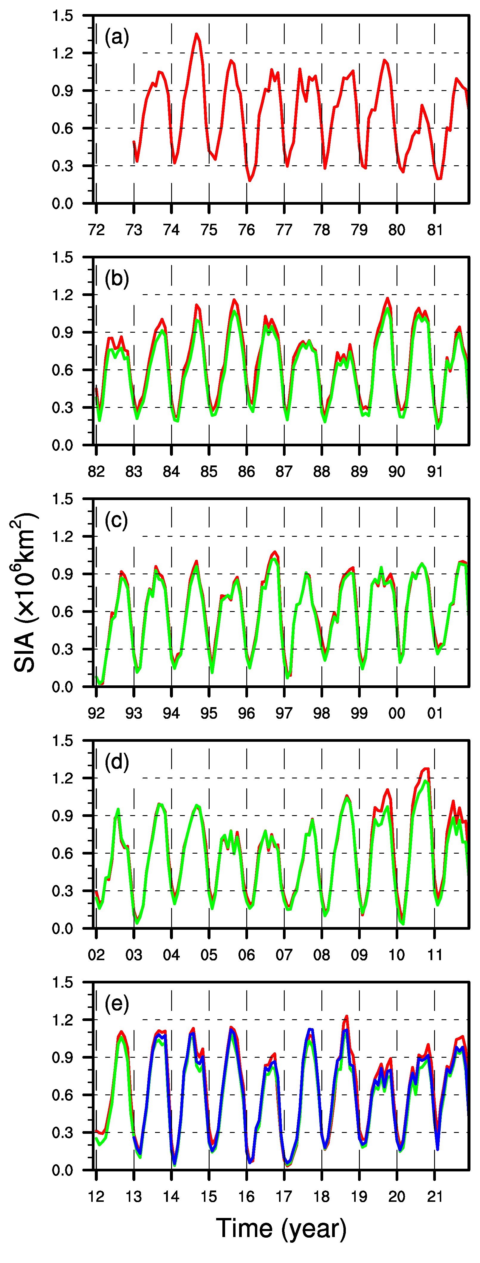
Figure 3.
Mean state of SIC in the Amundsen Sea (units: %; climatological annual mean). (a) HadISST1 (1982–2021), (b) OSTIA (1982–2021), (c) AMSR2 (2013–2021), (d) OSTIA (2013–2021), (e) HadISST1-OSTIA (1982–2021), and (f) AMSR2-OSTIA (2013–2021).
Figure 3.
Mean state of SIC in the Amundsen Sea (units: %; climatological annual mean). (a) HadISST1 (1982–2021), (b) OSTIA (1982–2021), (c) AMSR2 (2013–2021), (d) OSTIA (2013–2021), (e) HadISST1-OSTIA (1982–2021), and (f) AMSR2-OSTIA (2013–2021).
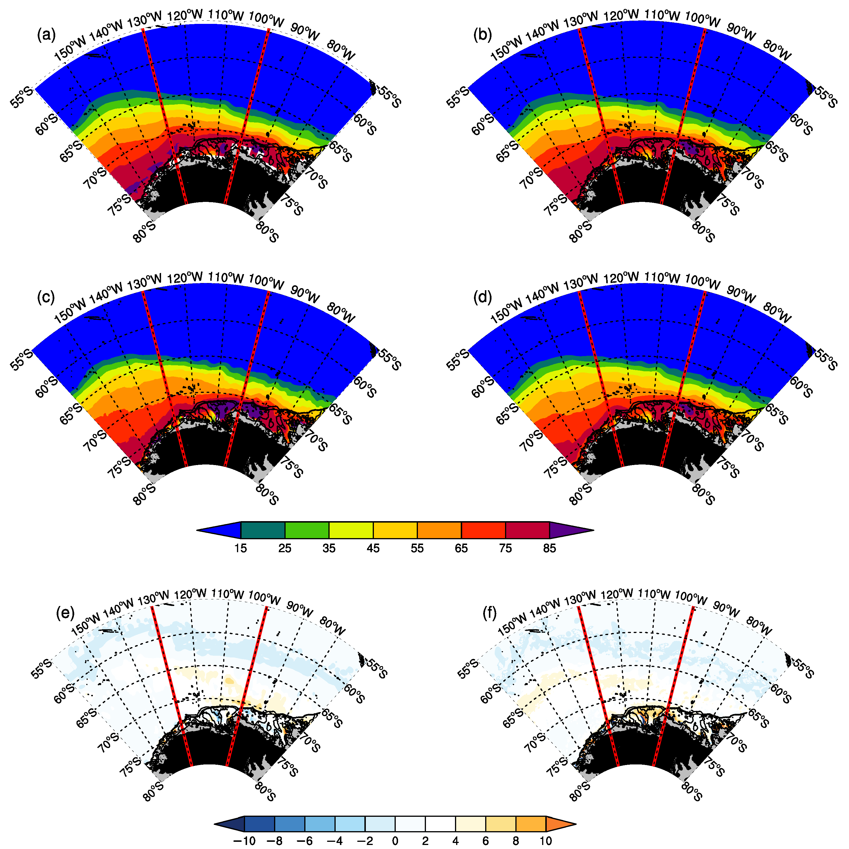
Figure 4.
Trend of SIC (units: %/decade). (a) HadISST1 (1982–2021), (b) OSTIA (1982–2021) and (c) AMSR2 (2013–2021). Annual mean SIC is used in computation. Black dots mean passing the 90% significance test.
Figure 4.
Trend of SIC (units: %/decade). (a) HadISST1 (1982–2021), (b) OSTIA (1982–2021) and (c) AMSR2 (2013–2021). Annual mean SIC is used in computation. Black dots mean passing the 90% significance test.
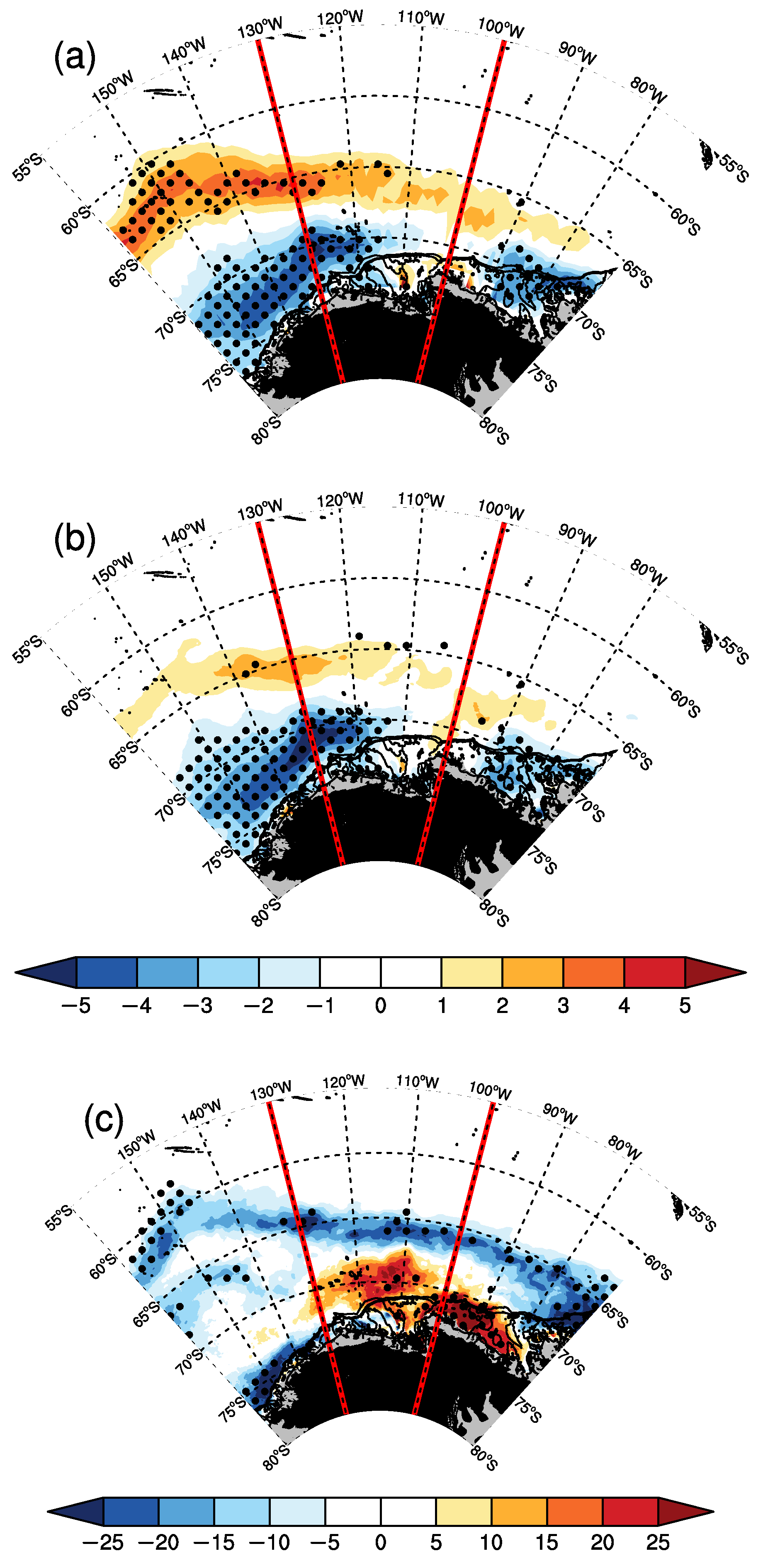
Figure 5.
Dacadal variation in SIA. Four decadal segments are selected as 8592 (1986–1992), 9398 (1993–1998), 99A4 (1999–2004), and A5B0 (2005–2011).
Figure 5.
Dacadal variation in SIA. Four decadal segments are selected as 8592 (1986–1992), 9398 (1993–1998), 99A4 (1999–2004), and A5B0 (2005–2011).
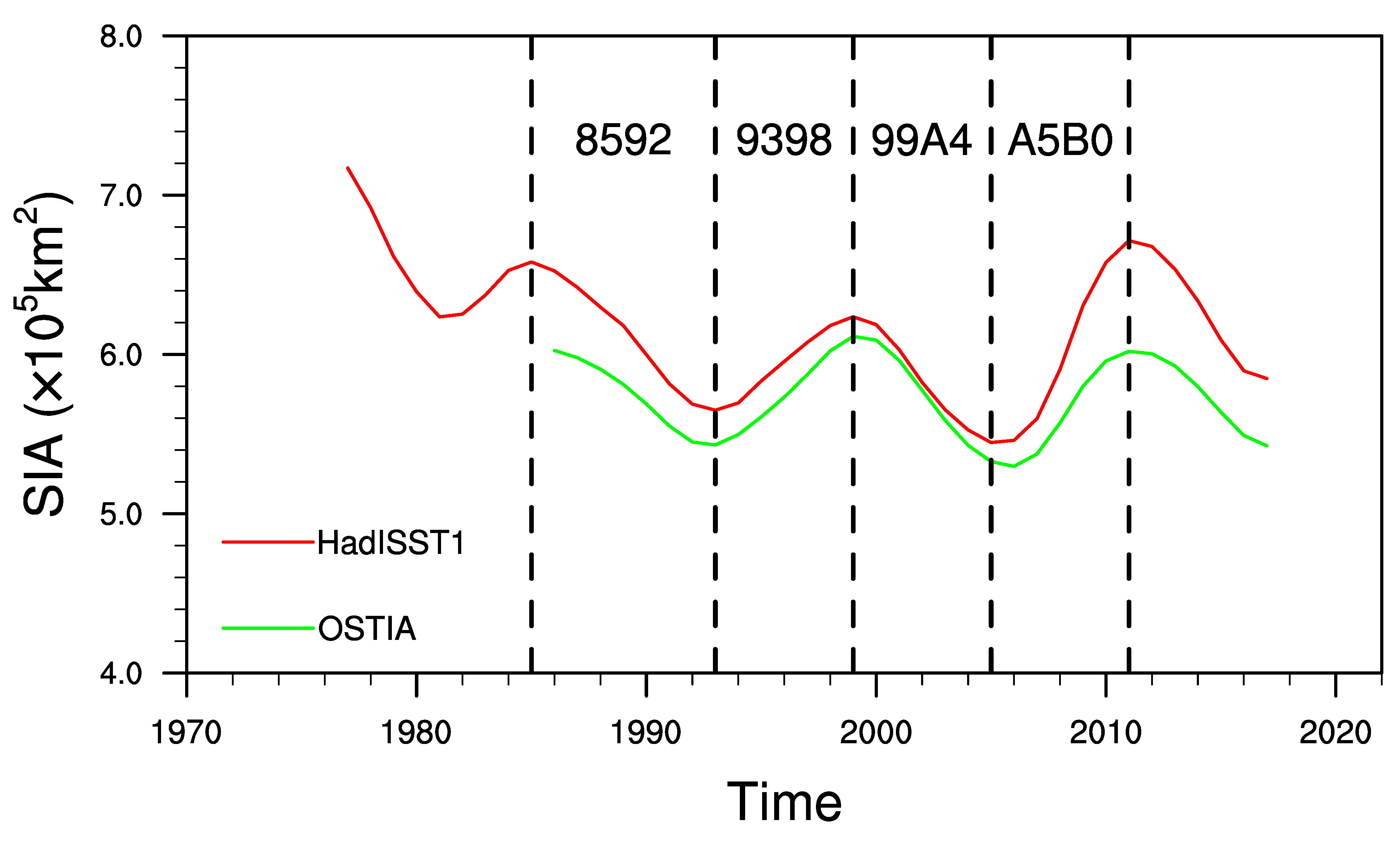
Figure 6.
Decadal trend in different periods (units: %/decadal). (a,b) 8592 (1985-1992), (c,d) 9398 (1993–1998), (e,f) 99A4 (1999–2004), and (g,h) A5B0 (2005–2010). (a,c,e,g) HadISST1; (b,d,f,h) OSTIA. Black dots mean passing the 90% significance test.
Figure 6.
Decadal trend in different periods (units: %/decadal). (a,b) 8592 (1985-1992), (c,d) 9398 (1993–1998), (e,f) 99A4 (1999–2004), and (g,h) A5B0 (2005–2010). (a,c,e,g) HadISST1; (b,d,f,h) OSTIA. Black dots mean passing the 90% significance test.
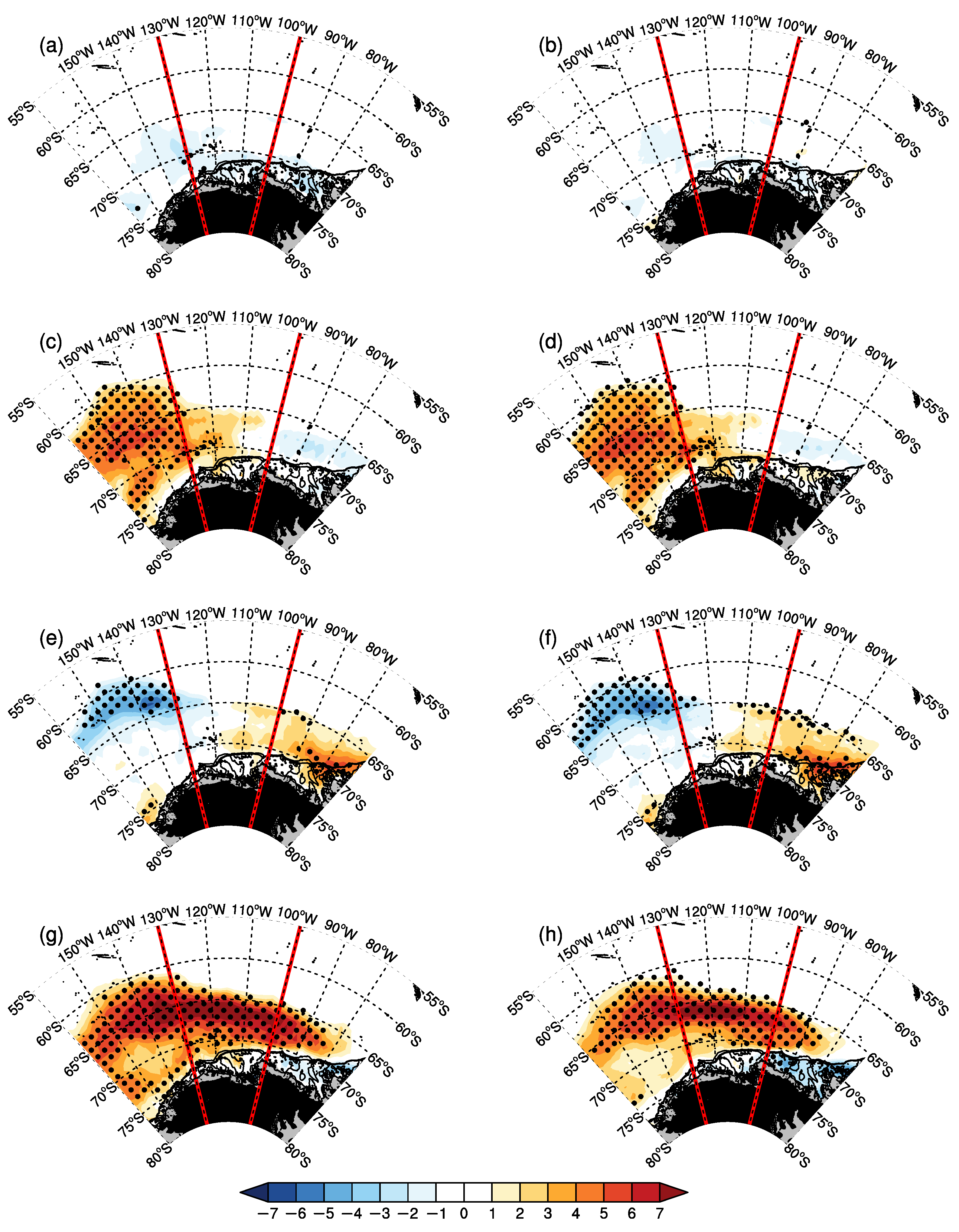
Figure 7.
Interannual variation in SIC (units: %). (a) HadISST1 (1982–2021), (b) OSTIA (1982–2021), and (c) AMSR2 (2013–2021). Standard deviations of SIC are shown. For HadISST1 and OSTIA, the results are obtained using bandpass filters between 2 and 8 years. Annual mean SIC is used in computation.
Figure 7.
Interannual variation in SIC (units: %). (a) HadISST1 (1982–2021), (b) OSTIA (1982–2021), and (c) AMSR2 (2013–2021). Standard deviations of SIC are shown. For HadISST1 and OSTIA, the results are obtained using bandpass filters between 2 and 8 years. Annual mean SIC is used in computation.

Figure 8.
Seasonal variation in SIC (units: %). (a,b) HadISST1 (1982–2021), (c,d) OSTIA (1982–2021), and (e,f) AMSR2 (2013–2021). Left panels (a,c,e) are SIC in winter (August). Right panels (b,d,f) are SIC in summer (February). Monthly mean SIC is used in computation.
Figure 8.
Seasonal variation in SIC (units: %). (a,b) HadISST1 (1982–2021), (c,d) OSTIA (1982–2021), and (e,f) AMSR2 (2013–2021). Left panels (a,c,e) are SIC in winter (August). Right panels (b,d,f) are SIC in summer (February). Monthly mean SIC is used in computation.

Figure 9.
Time series of Amundsen Sea polynya (ASP) area. (a) 1972–1982; (b) 1982–1992; (c) 1992–2002; (d) 2002–2012; and (e) 2012–2022. Three datasets are considered as HadISST1 (red line), OSTIA (green line), and AMSR2 (blue line). Abscissa axis is the time, where 72–99 represents 1972–1999, 00–21 indicates 2000–2021.


Table 1.
Satellite products of SICs.
| Dataset | Period | Period Used | Spatial Resolution | Temporal Resolution |
|---|---|---|---|---|
| HadISST | 1973/01 –present | 1973/01–2021/12 | 1 × 1 | monthly |
| OSTIA | 1981/10–present | 1982/01–2021/12 | 1/20 × 1/20 | daily |
| AMSR2 | 2012/08–present | 2013/01–2021/12 | 3.125 km × 3.125 km 1 | daily |
1 3.125 km × 3.125 km is nearly 0.03× 0.07.
Disclaimer/Publisher’s Note: The statements, opinions and data contained in all publications are solely those of the individual author(s) and contributor(s) and not of MDPI and/or the editor(s). MDPI and/or the editor(s) disclaim responsibility for any injury to people or property resulting from any ideas, methods, instructions or products referred to in the content. |
© 2023 by the authors. Licensee MDPI, Basel, Switzerland. This article is an open access article distributed under the terms and conditions of the Creative Commons Attribution (CC BY) license (https://creativecommons.org/licenses/by/4.0/).
Share and Cite
MDPI and ACS Style
Li, X.; He, H. Inter-Comparison of Satellite-Based Sea Ice Concentration in the Amundsen Sea, Antarctica. Remote Sens. 2023, 15, 5695. https://doi.org/10.3390/rs15245695
AMA Style
Li X, He H. Inter-Comparison of Satellite-Based Sea Ice Concentration in the Amundsen Sea, Antarctica. Remote Sensing. 2023; 15(24):5695. https://doi.org/10.3390/rs15245695
Chicago/Turabian StyleLi, Xueqi, and Hailun He. 2023. "Inter-Comparison of Satellite-Based Sea Ice Concentration in the Amundsen Sea, Antarctica" Remote Sensing 15, no. 24: 5695. https://doi.org/10.3390/rs15245695
Note that from the first issue of 2016, this journal uses article numbers instead of page numbers. See further details here.