Combining Texture, Color, and Vegetation Index from Unmanned Aerial Vehicle Multispectral Images to Estimate Winter Wheat Leaf Area Index during the Vegetative Growth Stage

Abstract

Leaf Area Index (LAI) is a fundamental indicator of plant growth status in agronomy and environmental research. With the rapid development of drone technology, the estimation of crop LAI based on drone imagery and vegetation indices is becoming increasingly popular. However, there is still a lack of detailed research on the feasibility of using image texture to estimate LAI and the impact of combining texture indices with vegetation indices on LAI estimation accuracy. In this study, two key growth stages of winter wheat (i.e., the stages of green-up and jointing) were selected, and LAI was calculated using digital hemispherical photography. The feasibility of predicting winter wheat LAI was explored under three conditions: vegetation index, texture index, and a combination of vegetation index and texture index, at flight heights of 20 m and 40 m. Two feature selection methods (Lasso and recursive feature elimination) were combined with four machine learning regression models (multiple linear regression, random forest, support vector machine, and backpropagation neural network). The results showed that during the vegetative growth stage of winter wheat, the model combining texture information with vegetation indices performed better than the models using vegetation indices alone or texture information alone. Among them, the best prediction result based on vegetation index was RFECV-MLR at a flight height of 40 m (R² = 0.8943, RMSE = 0.4139, RRMSE = 0.1304, RPD = 3.0763); the best prediction result based on texture index was RFECV-RF at a flight height of 40 m (R² = 0.8894, RMSE = 0.4236, RRMSE = 0.1335, RPD = 3.0063); and the best prediction result combining texture and index was RFECV-RF at a flight height of 40 m (R² = 0.9210, RMSE = 0.3579, RRMSE = 0.1128, RPD = 3.5575). The results of this study demonstrate that combining vegetation indices and texture from multispectral drone imagery can improve the accuracy of LAI estimation during the vegetative growth stage of winter wheat. In addition, selecting a flight height of 40 m can improve efficiency in large-scale agricultural field monitoring, as this study showed that drone data at flight heights of 20 m and 40 m did not significantly affect model accuracy.

1. Introduction

As a fundamental variable in agronomic and environmental studies, leaf area index (LAI) is often used as a key biophysical indicator of vegetation [1]. LAI is widely used in the study of plant photosynthesis [2], nitrogen fertilizer management [3] and water use [4]. LAI also plays a crucial role in practical applications of precision agriculture, including crop growth diagnostics, biomass estimation, and yield prediction. Wheat, as a vital component of the global human diet, provides a substantial source of carbohydrates, proteins, and fiber. Hence, the timely and accurate monitoring of winter wheat LAI information holds significant importance for its growth management and production forecasting.

Traditional methods for studying seasonal variations in vegetation LAI primarily involve direct and optical instrument-based approaches, which rely on intermittent LAI data for seasonal dynamics analysis [5]. Direct methods of measurement include destructive sampling, litterfall method, and point-quadrat method. They are relatively accurate but require a large amount of work and time, are labor-intensive, and can cause damage to vegetation. They cannot obtain continuous LAI data for the same vegetation. Indirect methods utilize optical principles to obtain LAI, with common instruments including LAI-2200, AccuPAR, SunScan, and TRAC, offering advantages such as ease of operation and non-destructiveness. In contrast to more expensive instruments, the fisheye camera method (DHP) is widely used due to its cost-effectiveness and ease of application [6]. However, the use of DHP is subject to external factors like weather and terrain, limiting its ability to collect continuous long-term LAI data. In summary, both direct and indirect methods have various limitations and are unable to provide spatial distribution information for LAI at a regional scale.

On the other hand, satellite platforms provide extensive remote sensing (RS) data. Remote sensing data can capture the reflectance of crop canopies, leading to widespread research on rapid and non-destructive LAI estimation at different perceptual scales using RS technology [7]. However, precision management during the growth season requires a large amount of timely multi-temporal data, and satellites are often constrained by factors such as revisit cycles and weather conditions, making it difficult to obtain a sufficient quantity of high-quality satellite data across multiple crop growth stages.

In recent years, the development of Unmanned Aerial Vehicles (UAVs) and their applications in remote sensing have provided new solutions for LAI estimation. Due to their flexibility in data acquisition and higher temporal and spatial resolutions, the use of UAV platforms for LAI research has gained widespread attention in the global academic community. For example, Zhu et al. [8] investigated lookup tables based on reflectance and vegetation indices at individual growth stages of wheat. Zhu et al. [8] evaluated the performance of different lookup tables for LAI retrieval in wheat. Lee et al. [9] used UAV imagery to estimate rice growth and found no significant correlation between LAI and vegetation indices after rice heading, indicating the challenge of establishing an LAI model that is applicable to multiple growth stages. Gong et al. [10] used several common vegetation indices based on drone imaging and found that using the product of vegetation index and canopy height can estimate LAI throughout the entire rice growing season. Unfortunately, the estimation error of the model reached 24%, and Gong et al. [10] did not consider the influence of drone flight altitude. Zhang et al. [11] established a general model for the jointing stage, heading stage, and grain-filling stage of winter wheat based on UAV hyperspectral data. Zhang’s research considered both the vegetative growth stage (jointing stage) and reproductive growth stage (heading stage and grain-filling stage) of wheat, showing strong applicability. However, Zhang’s study did not reflect the significant changes in LAI during the entire growth period of wheat (from the greening stage to the jointing stage), and Zhang et al. [11] also did not consider the influence of UAV flight altitude.

The above studies indicate that research on crop LAI using UAV platforms has garnered attention, but there is still a lack of remote sensing monitoring research on LAI throughout the entire vegetative growth period of crops. In addition, the choice of UAV flight altitude when utilizing UAVs for crop LAI estimation was not explored in previous studies, and most of the altitude choices in the existing studies were single and always empirically determined. Different UAV flight altitudes are closely related to the endurance time of the UAV and the estimation accuracy of the model, so the selection of different flight altitudes is necessary.

Estimating LAI based on spectral information is the approach used in most studies, and does not fully exploit UAV image information. In remote sensing science, the combination of spectral and texture information is complementary, providing rich information, enhancing classification accuracy, and interpreting image content [12]. Texture information has a close relationship with crop LAI [13].

Texture analysis is an image processing technique used to measure the variability in pixel values between adjacent pixels within a defined analysis window. It was initially applied in image classification and forest biomass estimation [14] in remote sensing images. Later, based on the texture information of remote sensing images, research on forest leaf area index (LAI) was conducted. Pu et al. [15] proposed a pixel-based seasonal LAI regression model using four seasonal Pleiades satellite images and corresponding LAI measurements, selecting a set of selected spectral and texture features. Pu and Cheng et al. [16] found that texture-based features extracted from the same WorldView-2 data had a better ability to estimate and map forest LAI compared to spectral-based features. Bolivar-Santamaria et al. [17] combined field vegetation structure measurements with Sentinel-2 images and used spectral and texture variables derived from Sentinel-2 images to predict LAI. The above studies explored the correlation of forest LAI based on satellite image texture information. Texture information has also been studied in crop growth monitoring. Eckert et al. [13] found that combining spectral features and texture measurements improved biomass estimation compared to using spectral or texture measurements alone. Zheng et al. [18] mounted a six-band spectral camera on an unmanned aerial vehicle (UAV) for rice biomass estimation. Zheng et al. [18] demonstrated that the Normalized Difference Texture Index (NDTI) based on the mean texture of the 550 nm and 800 nm band images outperformed the other texture variables and spectral indices. Subsequently, more studies demonstrated that texture predicted biomass better than spectral variables [19,20]. However, there have been few studies on the use of texture information from UAV multispectral images to estimate crop LAI.

The green-up and jointing stages correspond to the 25–30 and 30–32 stages of the Zadoks [21] scale, respectively. The green-up stage is the second tillering peak of winter wheat, and the jointing stage is a critical period for wheat’s vegetative growth, reproductive growth, and spike differentiation. During the entire reproductive period of winter wheat, the green-up and jointing stages are one of the most significant periods in which the leaf area index changes. In the middle and lower reaches of the Yangtze River, the phenomenon of ‘late spring cold’ occurs frequently [22], the leaves of winter wheat will suffer damage due to the lowering temperature, and large areas of yellowing and wilting may appear. The decrease in the leaf area index of winter wheat seriously affects the crop’s conversion of sunlight energy and its nitrogen utilization efficiency, which in turn affects the future growth rate and final yield of wheat. In this study, we chose this stage (green-up and jointing), and the objective was to explore the predictive performance of the UAV multispectral image-based vegetation index and texture features in winter wheat LAI estimation by collecting UAV multispectral data and wheat canopy hemispherical photography at different flight altitudes. In turn, different feature selection methods were combined with different machine learning algorithms to construct a model that is suitable for LAI estimation of winter wheat at the vegetative growth stage. In addition, to improve the generalization ability of the model, several wheat varieties were introduced to the study.

2. Materials and Methods

2.1. Experimental Site and Design

During the winter of 2022–2023, we conducted our study at the Integrated Demonstration Base of Modern Agricultural Science and Technology in Jiangyan District, Taizhou City, Jiangsu Province, China. The demonstration site is in the middle and lower reaches of the Yangtze River, with a flat topography, and is where the ‘late spring cold’ phenomenon occurs. The study area was divided into 72 plots (as shown in Figure 1), each with a planting area of 12 m² and a planting spacing of 25 cm between rows, of which 24 plots were used for experiment I and the remaining 48 plots were used for experiment II. Both experiments focused on the management of nitrogen fertilizer in winter wheat, and the method of nitrogen fertilizer application and treatment protocols were the differences between these two experiments.

The first 24 plots (Experiment 1) focused on the growth of winter wheat under different methods of N fertilizer application. The wheat varieties were Yangmai 39 (YM 39) and Yangmai 22 (YM 22). Urea and resin-coated urea were selected for nitrogen fertilizer, and the four different methods of nitrogen fertilizer application were spreading application, inter-row mix, inter-row application, and inter-row mix. The fertilizer application rate was 240 kg per hectare. The application rate of N fertilizer was 240 kg/ha. The experiment was conducted in a split-zone design with variety as the main block, fertilizer type as the sub-block, and fertilizer application method as the sub-sub-block. The experiment was conducted using different wheat varieties and different fertilizer types according to the different fertilizer application methods, with three replications, and the target plant density was set at 240,000 plants per hectare. Others were managed as per standard cultivation.

The latter 48 plots (Experiment II) were planted with four varieties of wheat: Yangmai 25 (YM 25), YM 39, Ningmai 26 (NM 26) and YM 22. Different wheat varieties have different nitrogen utilization efficiencies (YM 22 and NM 26 are nitrogen-inefficient utilizers, and YM 25 and YM 39 are nitrogen-efficient utilizers). This leads to strong differences in leaf area index at all growth stages of these four winter wheat varieties. These findings will have a positive impact on the generalizability of the research results. During the experiment, four different nitrogen fertilizer treatments of 0 kg/ha, 150 kg/ha, 240 kg/ha and 330 kg/ha were used. The experiment was replicated three times for different nitrogen fertilizer treatments. Nitrogen fertilizer was applied in the ratio of 5:1:2:2 in accordance with the base, tillering, jointing, and heading fertilizers, respectively. The basal fertilizer is applied before rotary tillage and sowing, the tillering fertilizer is applied when wheat grows to the three-leaf stage, and the jointing fertilizer is applied when wheat leaf residue reaches 2.5. The tasseling fertilizer is applied when wheat leaf residue drops to 0.8. Phosphorus and potash fertilizers were applied in the form of P₂O₅ and K₂O, and, for all treatment groups, pure phosphorus, and potassium were applied at a rate of 135 kg per hectare and applied as a one-time basal fertilizer. In the experiment, wheat was planted with a 25 cm inter-row spacing using manual furrow sowing. The area of each plot was 12 m² and the experiment was replicated three times. Plant counts were conducted when the wheat reached the two-leaf stage to achieve the target plant density of 240,000 plants per hectare. Other field management practices followed standard farm practices.

2.2. Data Collection and Processing

2.2.1. UAV Image Acquisition and Processing

A DJI P4M drone was chosen for the experiment, which can collect reflectance in five bands (Blue (B), Green (G), Red (R), Rededge and Near Infrared (NIR)). Unlike common RGB cameras on the market, the DJI P4M drone camera carries five spectral bands to provide a basis for calculating commonly used vegetation indices, while data collection was carried out in the morning with clear weather to avoid cloud shadows and shadows in the multispectral images. Route planning was performed with DJI Ground Station Pro 2.0 software (https://www.dji.com/cn/ground-station-pro (accessed on 17 May 2023)). Two diffuse reflectance standard plates representing 0.5 and 0.75 were placed on the ground before takeoff for radiometric calibration. The specific settings of the UAV flight parameters are shown in

Table A1. Settings of UAV flight parameters.

Parameters	Setting 1	Setting 2
Flight altitude	20 m	40 m
Flight speed	3 m/s	3 m/s
Heading overlap rate	80%	80%
Sideways overlap	80%	80%
Resolution	1.06 cm	2.12 cm

in Appendix A. After the flight was completed, we processed the images using DJI Terra 2.3 software (https://enterprise.dji.com/cn/dji-terra (accessed on 22 May 2023)) to produce a final single-band reflectance image. Based on the UAV acquisition content, the images were categorized using eCognition 9.0 software (https://geospatial.trimble.com/en (accessed on 19 May 2023). The images were categorized into soil, shadow, and vegetation, and the same categories were merged and masked for soil using ArcMap (ESRI Inc.; Redlands, CA, USA).

2.2.2. Field Leaf Area Index Measurement

The measurement of the Green Plant Area Index (PAI) for the winter wheat canopy was conducted on the same day as the acquisition of the UAV multispectral images. PAI was determined using the Digital Hemispherical Photography (DHP) method. DHP is known for its simplicity, non-destructive nature, and wide application in vegetation studies. Shang et al. [6], for example, used DHP to assess the spatiotemporal variation in crop growth PAI while studying the interactions between plants and environmental conditions. Dong et al. [23], based on DHP measurements of LAI for spring wheat and rapeseed, developed a universal LAI estimation algorithm using red-edge vegetation indices for different crops. In the field measurements, a 10.5 mm fisheye lens and a Nikon D7500 camera were used to capture canopy images. The Nikon D7500 can be equipped with a fisheye lens, which has a very wide field of view, a prerequisite for the digital hemispherical photography method of calculating crop LAI. During each sampling event, uniform photos were taken over the winter wheat canopy. Given the relatively low height of the wheat canopy during the study period, the camera lens was positioned 0.5 m above the canopy, facing downward [24]. Fourteen photos were taken for each experimental plot during the data collection process, ensuring full coverage of the plot. These images were processed in the laboratory using the CanEye 6.495 software [25], which was used to calculate both the Effective Plant Area Index (PAI) and the Total Plant Area Index (PAI). Total PAI is defined as half of the total surface area of plant tissue per unit ground area [26,27]. For wheat, the Green Effective PAI is equivalent to the Leaf Area Index (LAI).

2.2.3. Extracting Texture and Vegetation Indices

In this study, 40 common vegetation indices were selected to estimate the leaf area index (LAI) (Table 1). These indices provide information on vegetation growth, health, etc., such as the Normalized Vegetation Index (NDVI), calculated using reflectance values between the infrared and visible bands, where higher values indicate more lush vegetation; the Green Chlorophyll Index (Cigreen) calculated using reflectance values between the green and red bands correlates with the chlorophyll content because of the relatively high absorption of green light by chlorophyll; and the Optimized Soil Adjusted Vegetation Index (OSAVI), a variant of the Soil Adjusted Vegetation Index (OSAI), which is more likely to provide stable results in areas with highly variable soil types.

Common texture indices, which include contrast, correlation, energy, and homogeneity, were computed based on the Gray-Level Co-occurrence Matrix (GLCM). GLCM is a classic method introduced by Haralick et al. [28] in 1973 for extracting texture features. These texture indices were independently extracted for each sample area based on GLCM, computed for their average characteristics, and the temporal variations of different growth stages’ texture indices were obtained. In this study, eight texture features were extracted from the multispectral images using the “Co-occurrence Measures” function in ENVI 5.3 software, including mean (ME), variance (VA), homogeneity (HO), contrast (CO), dissimilarity (DI), entropy (EN), second moment (SE), and correlation (COR) (

Table 2. Eight texture variables used for LAI estimation in this study.

Textural Indices	Formula	Reference
Mean	${\mu }_i=i{\displaystyle {\displaystyle \sum }_{ij=0}^{N-1}}{P}_{ij};{\mu }_j=j{\displaystyle {\displaystyle \sum }_{ij=0}^{N-1}}{P}_{ij}$	[28]
Variance	${\sigma }_i^2={{\displaystyle \sum }}_{i,j=0}^{N-1}{P}_{ij}{\left(i-{\mu }_i\right)}^2;{\sigma }_j^2={{\displaystyle \sum }}_{i,j=0}^{N-1}{P}_{ij}{\left(j-{\mu }_j\right)}^2$	[28]
Homogeneity	${\displaystyle {\displaystyle \sum }_{i,j=0}^{N-1}}\frac{P_{i,j}}{1+{\left(i-j\right)}^2}$	[28]
Contrast	${\displaystyle {\displaystyle \sum }_{i,j=0}^{N-1}}{P}_{i,j}{\left(i-j\right)}^2$	[28]
Dissimilarity	${\displaystyle {\displaystyle \sum }_{i,j=0}^{N-1}}{P}_{i,j}\left|i-j\right|$	[28]
Entropy	${\displaystyle {\displaystyle \sum }_{i,j=0}^{N-1}}{P}_{i,j}(-\ln P_{i,j})$	[28]
Second Moment	${\displaystyle {\displaystyle \sum }_{i,j=0}^{N-1}}{P}_{i,j}$	[28]
Correlation	${\displaystyle {\displaystyle \sum }_{i,j=0}^{N-1}}{P}_{i,j}\frac{\left(i-{\mu }_i\right)(j-{\mu }_j)}{1+{\left(i-j\right)}^2}$	[28]

). A window size of 7 × 7 was chosen based on previous research [29] and multiple trials to ensure clear differentiation between soil and wheat pixels, while other parameters were kept at their default values.

Table 1. Forty spectral variables used for LAI estimation in this study.

NO.	VI	Formula	Reference
1	R	R	-
2	G	G	-
3	B	B	-
4	NIR	NIR	-
5	Rededge	Rededge	-
6	INT	(R + G + B)/3	[30]
7	IKAW	(R − B)/(R + B)	[31]
8	IPCA	0.994|R − B| + 0.961|G − B| + 0.914|G − R|	[32]
9	ExR	1.4R − G	[33]
10	ExG	2G − R − B	[34]
11	ExGR	2G − R − B − (1.4R − G)	[33]
12	MGRVI	(G2 − R2)/(G2 + R2)	[35]
13	RGBVI	(G2 − B × R)/(G2 + B × R)	[35]
14	NDVI	(NIR − R)/(NIR + R)	[36]
15	GNDVI	(NIR − G)/(NIR + G)	[37]
16	RVI	(NIR/R)	[38]
17	NDREI	(NIR − RE)/(NIR + RE)	[39]
18	EVI	2.5 × (NIR − R)/(1 + NIR − 2.4 × R)	[40]
19	OSAVI	(NIR − R)/(NIR − R + 0.16)	[41]
20	MCARI	[(RE − R) − 0.2 × (RE − G)] × (RE/R)	[42]
21	TCARI	3 × [(RE − R) − 0.2 × (RE − G) × (RE/R)]	[43]
22	NRI	(G − R)/(G + R)	[44]
23	TVI	Sqrt (NDVI + 0.5)	[45]
24	MSR	((NIR/R) − 1) × sqrt (NIR/R + 1)	[46]
25	SIPI	(NIR − B)/(NIR + B)	[47]
26	PSRI	(R − B)/NIR	[48]
27	CI_re	NIR/R − 1	[49]
28	SAVI	(NIR − R)/(NIR + R + 0.5) × 1.5	[50]
29	CRI	1/G + 1/NIR	[51]
30	NLI	(NIR × NIR − R)/(NIR × NIR + R)	[52]
31	RDVI	(NIR − R)/sqrt (NIR + R)	[53]
32	CI_green	NIR/G − 1	[49]
33	MTCI	(NIR − RE)/(RE − R)	[54]
34	MTVI1	1.2[1.2(NIR − G) − 2.5(R − G)]	[55]
35	MTVI2	(1.5 × (1.2(NIR − G) − 2.5(R − G)))/sqrt((2 × NIR + 1)2 − (6 × NIR − 5 × sqrt(R)) − 0.5)	[55]
36	VARI	(G − R)/(G + R − B)	[49]
37	ExB	1.4 × B − G	[56]
38	WI	(G − B)/(R − G)	[34]
39	GLA	(2 × G − R − B)/(2 × G + R + B)	[36]
40	VEG	G/RaB(1−a), a = 0.667	[57]

Note: B, G, R, rededge, and NIR are the raw values for the five bands of the UAV.

Table 1. Forty spectral variables used for LAI estimation in this study.

NO.	VI	Formula	Reference
1	R	R	-
2	G	G	-
3	B	B	-
4	NIR	NIR	-
5	Rededge	Rededge	-
6	INT	(R + G + B)/3	[30]
7	IKAW	(R − B)/(R + B)	[31]
8	IPCA	0.994|R − B| + 0.961|G − B| + 0.914|G − R|	[32]
9	ExR	1.4R − G	[33]
10	ExG	2G − R − B	[34]
11	ExGR	2G − R − B − (1.4R − G)	[33]
12	MGRVI	(G2 − R2)/(G2 + R2)	[35]
13	RGBVI	(G2 − B × R)/(G2 + B × R)	[35]
14	NDVI	(NIR − R)/(NIR + R)	[36]
15	GNDVI	(NIR − G)/(NIR + G)	[37]
16	RVI	(NIR/R)	[38]
17	NDREI	(NIR − RE)/(NIR + RE)	[39]
18	EVI	2.5 × (NIR − R)/(1 + NIR − 2.4 × R)	[40]
19	OSAVI	(NIR − R)/(NIR − R + 0.16)	[41]
20	MCARI	[(RE − R) − 0.2 × (RE − G)] × (RE/R)	[42]
21	TCARI	3 × [(RE − R) − 0.2 × (RE − G) × (RE/R)]	[43]
22	NRI	(G − R)/(G + R)	[44]
23	TVI	Sqrt (NDVI + 0.5)	[45]
24	MSR	((NIR/R) − 1) × sqrt (NIR/R + 1)	[46]
25	SIPI	(NIR − B)/(NIR + B)	[47]
26	PSRI	(R − B)/NIR	[48]
27	CI_re	NIR/R − 1	[49]
28	SAVI	(NIR − R)/(NIR + R + 0.5) × 1.5	[50]
29	CRI	1/G + 1/NIR	[51]
30	NLI	(NIR × NIR − R)/(NIR × NIR + R)	[52]
31	RDVI	(NIR − R)/sqrt (NIR + R)	[53]
32	CI_green	NIR/G − 1	[49]
33	MTCI	(NIR − RE)/(RE − R)	[54]
34	MTVI1	1.2[1.2(NIR − G) − 2.5(R − G)]	[55]
35	MTVI2	(1.5 × (1.2(NIR − G) − 2.5(R − G)))/sqrt((2 × NIR + 1)2 − (6 × NIR − 5 × sqrt(R)) − 0.5)	[55]
36	VARI	(G − R)/(G + R − B)	[49]
37	ExB	1.4 × B − G	[56]
38	WI	(G − B)/(R − G)	[34]
39	GLA	(2 × G − R − B)/(2 × G + R + B)	[36]
40	VEG	G/RaB(1−a), a = 0.667	[57]

Note: B, G, R, rededge, and NIR are the raw values for the five bands of the UAV.

2.3. Feature Variable Screening

Feature selection is particularly important when there is a high degree of correlation among features. Highly correlated features can introduce multicollinearity issues. Therefore, two effective feature selection methods were employed in this study, namely L1 regularization Least Absolute Shrinkage and Selection Operator (Lasso) and Recursive Feature Elimination (RFE).

While in ordinary least squares regression, the objective is to fit the model parameters by minimizing the squared error between the actual observations and the predicted values, Lasso’s [58] regression introduces an additional L1 penalty into the objective function (the second term in Equation (1), the first term being the objective function of ordinary least squares). With the L1 penalty, the tendency is to set the coefficients of the unimportant features to zero, thus automating feature selection. This can help prevent overfitting and improve the generalization ability of the model. Alpha parameter selection can then be set through cross-validation. Thus, Lasso effectively reduces the number of features on which a given solution depends, which is important in the field of compressed perception.

$$\underset{\omega }{\min }\frac{1}{2n_{samples}}{\Vert X_{\omega }-y\Vert }_2^2+\alpha {\Vert \omega \Vert }_1$$

(1)

The Recursive Feature Elimination (RFE) method [59] utilizes an external estimator that assigns weights to features and selects features by recursively considering smaller and smaller feature sets. Firstly, the estimator is trained on the initial feature set, and the importance of each feature is obtained through specific attributes or callable methods. Subsequently, the least important features are pruned from the current feature set. This process is recursively repeated on the pruned feature set until the desired number of selected features is achieved. The modeling process employed a cross-validated RFE methodology in which the ridge regression algorithm was used as the evaluation coefficient.

2.4. Machine Learning Regression Algorithms

In this study, models for estimating the Leaf Area Index (LAI) of winter wheat during its vegetative growth stages (green-up and jointing stages) were developed. At flight altitudes of 20 m and 40 m, feature selection was performed using two different methods on three different datasets. Subsequently, four different machine learning algorithms were employed to fit the data, resulting in a total of 48 regression models. The model parameters in the study (except for MLR) were constructed using a grid search combined with 5-fold cross-validation. The four algorithms used in the study were Multiple Linear Regression [60], Random Forest [61], Support Vector Machine [62], and Backpropagation Neural Network [63]. The first three of the four machine learning algorithms have been frequently used in previous studies and include linear models as well as nonlinear models. With the use of deep learning algorithms in the field of agriculture, back propagation neural networks were also chosen for fitting in this study so that the comparison and selection of different models can be carried out.

2.4.1. Multiple Linear Regression

Linear regression is a commonly used machine learning algorithm for prediction and modeling, employed to analyze the linear relationship between variables. The fundamental principle is to establish the relationship between input features and output targets by finding the best-fitting line (or plane). Multivariate linear regression (MLR, as shown in Equation (2)) is more than univariate regression; it takes full advantage of the practical application of multivariate inputs, and presents strong interpretability while having a simple form.

$$LAI={\beta }_0+{\beta }_1{X}_1+{\beta }_2{X}_2+{\beta }_3{X}_3+\cdots +{\beta }_n{X}_n$$

(2)

2.4.2. Random Forest

Random forests are composed of the autonomous resampling method (Bootstrap) proposed by Breiman et al. [61] and the random subspace method introduced by Kam et al. [64]. They find application in various tasks, such as classification, regression, and clustering. In Random Forest, decision trees are constructed using random subsets of the training data. The ensemble of multiple decision trees in Random Forest aggregates their prediction results through methods like voting or averaging. This aggregation yields more stable and accurate results, reducing the risk of model overfitting.

2.4.3. Support Vector Machine

Support Vector Machine (SVM) is proposed based on the principle of structural risk minimization. The application of SVM to regression prediction is called Support Vector Regression (SVR). To solve the nonlinear problem, SVR transforms the nonlinear problem into a linear problem in a high-dimensional space, and then uses a kernel function instead of the inner product operation in the high-dimensional space. The parameters of SVR include the “gamma” (kernel parameter) and C (penalty coefficient). In the study, a linear kernel function is used to find the optimal parameter C through a grid search.

2.4.4. Backpropagation Neural Network

In the groundbreaking paper published in 1986 by David Rumelhart, Geoffrey Hinton, and Ronald Williams [65], the backpropagation training algorithm was introduced. This algorithm provided significant assistance in training multilayer perceptrons and led to the rapid development of backpropagation neural networks. It is an efficient technique for automatically computing gradient descent. The backpropagation algorithm is capable of calculating the gradient of network error with respect to each model parameter in just two passes through the network (one forward pass and one backward pass). In other words, it can determine how each connection weight and bias should be adjusted to minimize the error. Once these gradients are obtained, it follows the standard gradient descent steps and repeats the entire process until the network converges to a solution. Backpropagation neural networks typically consist of an input layer, an output layer, and several hidden layers. Neurons in each layer are connected to neurons in the next layer, transmitting information. In each neuron, the output value of the previous layer of neurons is linearly weighted as the input value, which is processed by a nonlinear activation function and used as the input value of the next layer of neurons.

2.4.5. Cross-Validation and Grid Search

The main idea of cross-validation is to divide the dataset into K parts, where K-1 parts are used as the training set and the remaining 1 part is used as the validation set. In the study, the value of K was set to 5. Grid search is a method of tuning model parameters by exhaustive search and is usually combined with cross-validation to optimize model parameters. In selecting all candidate parameter combinations, the estimates of model CVs under each parameter combination were obtained by loop traversal, and the parameter combination with the best estimates was the final selected parameter. In the study, the RF model was optimized with the parameter “n-estimators”, the SVR model was optimized with the parameter “C”; the BP neural network model, the optimized parameters were “n-estimators” and “learning rate”.

2.5. Statistical Analysis

The post-data collection statistical analysis process is summarized in Figure 2’s flowchart. Samples with the same height from two periods were merged (n = 144), and the overall dataset was divided into training and testing datasets in an 8:2 ratio. Given the significant differences in winter wheat leaf area index under different nitrogen application levels, a stratified sampling approach was employed to partition the training and testing datasets. This was to avoid potential imbalances in sample counts for certain categories due to random sampling, which could affect model training and performance. Most features covering different experimental treatments were used to construct and fine-tune multiple regression models, including Multivariate Linear Regression (MLR), Random Forest (RF), Support Vector Machine Regression (SVM), and Backpropagation Neural Network (BPNN) regression models, using selected vegetation indices, texture, or a combination of both as inputs. Overfitting is prone to occur with a limited dataset. When the model adapts to the noise in the training data and the characteristics of a particular sample, the generalization performance of the model can be drastically reduced. Cross-validation can be employed to more comprehensively assess the model’s performance and generalization ability. The training process involved 5-fold cross-validation combined with grid search to find the optimal model hyperparameters and the final predictive performance was evaluated using the testing dataset. The evaluation metrics included the coefficient of determination, determined through cross-validation (R², Equation (3)), root mean square error (RMSE, Equation (4)), and relative root mean square error (rRMSE, Equation (5)). R² measures the extent to which the model explains the variability of the target variable, and its value ranges from 0 to 1. The closer it is to 1, the better the model fits the data. RMSE measures the difference between the model’s predicted value and the actual value; the smaller the value is, the better the model fits the data. The relative root–mean–square error (rRMSE) takes into account the scaling of the observations on top of the root–mean–square error (rRMSE) which makes the error metrics easier to interpret and compare. In addition, considering the balance between the predictive performance of the model and the variability of the data, the the ratio of the standard deviation of the measurements to the RMSE (RPD) was calculated in this paper. Rossel et al. [66] showed that a 1.8 ≤ RPD < 2.0 indicates that it can be used for general prediction tasks, 2.0 ≤ RPD < 2.5 indicates that it can be used for accurate prediction tasks, and RPD ≥ 2.5 indicates very high prediction accuracy.

$$R^2=1-\frac{{{\displaystyle \sum }}_{i=1}^n{\left(y_i-{\widehat{y}}_i\right)}^2}{{{\displaystyle \sum }}_{i=1}^n{(y_i-{\overline{y}}_i)}^2}$$

(3)

$$RMSE=\sqrt{\frac{1}{n}{{\displaystyle \sum }}_{i=1}^n{\left(y_i-{\widehat{y}}_i\right)}^2}$$

(4)

$$rRMSE=\sqrt{\frac{1}{n}{{\displaystyle \sum }}_{i=1}^n{\left(y_i-{\widehat{y}}_i\right)}^2}/\overline{y}$$

(5)

3. Results

3.1. Variability of Winter Wheat Leaf Area Index

The Leaf Area Index (LAI) of winter wheat exhibits significant variations, as anticipated, influenced by factors such as nitrogen fertilizer dosage, crop varieties, and growth stages (

Table 3. Descriptive statistics of Leaf Area Index (LAI) in the training and testing datasets.

Growth Stage	Samples	LAI
		Min	Max	Mean	SD	CV (%)
Training Dataset
Green-up and Jointing	115	0.56	5.52	3.38	1.12	34.07
Test Dataset
Green-up and Jointing	29	0.73	4.96	3.17	1.27	40.13

). Across the three principal growth stages encompassing the vegetative growth phases of winter wheat, both the training and testing datasets reveal an increasing LAI trend. In the training dataset, LAI values during the green-up and jointing growth stages range from 0.56 to 5.52, while in the testing dataset, the range extends from 0.73 to 4.96. Furthermore, substantial variability is observed in LAI during these two growth stages, indicating the potential coverage of a wide range of scenarios. This variability also renders the estimation of winter wheat LAI using remote sensing and unmanned aerial vehicle (UAV) data feasible.

3.2. Feature Selection

The heat map (Figure A1 in Appendix A) illustrates that during the vegetative growth stages of winter wheat, namely the green-up and jointing stages, there exists a high degree of correlation among some of the predictive factors, whether they are vegetation indices (VIs) or texture indices. This suggests a potential issue of overfitting when utilizing all VIs or texture indices. High correlations among features can diminish the interpretability of the model, making it challenging to understand the factors influencing predictions. Through feature selection, we can choose the most representative features, reduce feature dimensionality, and enhance both model interpretability and generalization performance.

When employing Lasso linear regression for feature selection, a crucial hyperparameter needs adjustment, namely the regularization parameter (also known as the penalty parameter), typically denoted as α (alpha). α controls the strength of the L1 regularization term, thereby influencing the feature selection process. A larger α value results in more feature coefficients becoming zero, thereby enhancing the effectiveness of feature selection, while a smaller α value reduces sparsity in feature coefficients, retaining more features in the model. There is no universal rule for selecting the alpha parameter, and it is determined based on cross-validation to minimize the root–mean–square error (Figure 3).

The Recursive Feature Elimination (RFE) method is based on the idea of iteratively removing features that contribute less to the model’s performance. In this study, ridge regression (RR) was selected as the evaluation criterion for RFE. The optimal number of predictive factors was determined based on cross-validation to minimize RMSE (Figure 4).

As shown in

Table 4. Variable selection results.

Variable	20 m						40 m
	Lasso			RFECV			Lasso			REFCV
	VI	TI	VI + TI	VI	TI	VI + TI	VI	TI	VI + TI	VI	TI	VI + TI
NIR				√
ExR	√						√
MGRVI	√			√					√			√
RGBVI				√		√				√
NDVI				√
GNDVI				√
NDREI				√
EVI				√
OSAVI							√		√
MCARI	√			√
TCARI				√		√
MSR				√
SAVI				√
NLI	√			√		√	√		√	√
RDVI				√
MTCI				√		√
MTVI1				√		√
GLA			√	√			√		√
VEG	√		√	√		√
r-mean		√	√		√			√	√		√
r-homogeneity											√
r-contrast					√						√
r-dissimilarity					√						√
r-entropy					√						√
r-second moment						√
r-correlation			√		√			√
g-mean					√
g-variance					√			√	√		√
g-homogeneity					√						√
g-contrast											√
g-dissimilarity					√						√
g-entropy					√						√
g-second moment					√	√					√
g-correlation								√	√		√	√
b-variance					√						√
b-homogeneity			√								√
b-contrast					√						√
b-dissimilarity			√								√
b-entropy						√
b-second moment			√
b-correlation					√	√					√
n-mean		√	√					√	√
n-variance		√	√
n-homogeneity											√
n-contrast		√
n-dissimilarity											√
n-entropy											√
n-correlation								√	√		√	√
re-dissimilarity											√
re-entropy					√
re-correlation											√

Note: The variables listed in the table are those selected through feature selection.

, after the Lasso feature selection method, at a flight height of 20 m, 5 spectral variables were retained and 4 texture variables were retained; for spectral variables plus texture variables, 9 were retained. At a flight height of 40 m, 4 spectral variables were retained and 6 texture variables were retained; for spectral variables plus texture variables, 9 were retained. After the RFECV feature selection method, at a flight height of 20 m, 17 spectral variables were retained and 15 texture variables were retained; for spectral variables plus texture variables, 10 were retained. At a flight height of 40 m, 2 spectral variables were retained and 23 for texture variables were retained; for spectral variables plus texture variables, 3 were retained.

Under different flight altitudes and feature selection methods, there are significant differences in the types and quantities of optimal variable selection. However, there are also some features that are not affected by flight altitude and feature selection methods in a single dataset. For example, texture indices r-mean and n-mean are selected multiple times under different altitudes and different feature selection methods. There are also some features that do not appear repeatedly, such as NIR and re-correlation, which are only selected once as optimal variables.

3.3. The Best Model for Predicting Winter Wheat LAI

3.3.1. The Best Model Based on Vegetation Indices

The model based on the vegetation index (

Table 5. Model results based on vegetation index-selected variables.

Height		Model	Train				Test
			R2	RMSE	RRMSE	RPD	R2	RMSE	RRMSE	RPD
20 m	Lasso	MLR	0.8664	0.4097	0.1246	2.7360	0.7129	0.6823	0.2150	1.8664
		RF	0.9171	0.3227	0.0981	3.4742	0.8912	0.4201	0.1324	3.0313
		SVM	0.8474	0.4379	0.1331	2.5599	0.7939	0.5781	0.1822	2.2028
		BPNN	0.8925	0.3774	0.1136	3.0500	0.6132	0.7655	0.2452	1.6078
	RFECV	MLR	0.8863	0.3780	0.1149	2.9657	0.6658	0.7361	0.2320	1.7299
		RF	0.9423	0.2692	0.0818	4.1638	0.8896	0.4231	0.1333	3.0095
		SVM	0.8711	0.4025	0.1223	2.7854	0.7845	0.5912	0.1863	2.1539
		BPNN	0.8646	0.4235	0.1275	2.7178	0.7568	0.6069	0.1944	2.0279
40 m	Lasso	MLR	0.8538	0.4286	0.1303	2.6153	0.8877	0.4268	0.1345	2.9837
		RF	0.9269	0.3031	0.0921	3.6982	0.8814	0.4385	0.1382	2.9041
		SVM	0.8493	0.4351	0.1323	2.5763	0.8812	0.4389	0.1383	2.9016
		BPNN	0.8688	0.4170	0.1255	2.7604	0.8688	0.4458	0.1428	2.7607
	RFECV	MLR	0.8512	0.4324	0.1315	2.5923	0.8943	0.4139	0.1304	3.0763
		RF	0.9002	0.3542	0.1077	3.1653	0.8710	0.4574	0.1441	2.7842
		SVM	0.8500	0.4342	0.1320	2.5819	0.8943	0.4140	0.1305	3.0759
		BPNN	0.8734	0.4096	0.1233	2.8104	0.8731	0.4384	0.1404	2.8076

Note: the best results are in bold.

) shows that the RF model and MLR model have the best predictive performance under different flight heights and feature selection methods. At a flight height of 20 m and with Lasso feature selection, the RF model performs as follows on the training set: R² = 0.9171, RPD = 3.4742, RMSE = 0.3227, and RRMSE = 0.0981. On the test set, R² = 0.8912, RPD = 3.0313, RMSE = 0.4201, and RRMSE = 0.1324. At a flight height of 40 m and with RFECV selection, the MLR model performs as follows on the training set: R² = 0.8512, RPD = 2.5923, RMSE = 0.4324, and RRMSE = 0.1315. On the test set, it performs as follows: R² = 0.8943, RPD = 3.0763, RMSE = 0.4139, and RRMSE = 0.1304. Specifically, when estimating the LAI of winter wheat during the vegetative growth stages (green-up stage and jointing stages) based on the vegetation index, the RFECV-MLR model at a flight height of 40 m is considered the best model.

3.3.2. The Best Model Based on Texture Indices

The model based on texture index (

Table 6. Model results based on texture index-selected variables.

Height		Model	Train				Test
			R2	RMSE	RRMSE	RPD	R2	RMSE	RRMSE	RPD
20 m	Lasso	MLR	0.8601	0.4193	0.1275	2.6736	0.8576	0.4805	0.1514	2.6501
		RF	0.9131	0.3304	0.1005	3.3923	0.8792	0.4426	0.1395	2.8770
		SVM	0.6174	0.6934	0.2108	1.6167	0.5426	0.8612	0.2714	1.4786
		BPNN	0.8810	0.3971	0.1195	2.8987	0.8313	0.5054	0.1619	2.4350
	RFECV	MLR	0.8908	0.3704	0.1126	3.0268	0.8757	0.4490	0.1415	2.8361
		RF	0.9284	0.3001	0.0912	3.7359	0.8785	0.4439	0.1399	2.8683
		SVM	0.8607	0.4183	0.1272	2.6797	0.8349	0.5174	0.1630	2.4613
		BPNN	0.8477	0.4492	0.1352	2.5627	0.8035	0.5456	0.1748	2.2559
40 m	Lasso	MLR	0.8871	0.3900	0.1223	2.9759	0.8293	0.4445	0.1244	2.4201
		RF	0.9381	0.2886	0.0905	4.0205	0.8471	0.4207	0.1177	2.5572
		SVM	0.6336	0.7025	0.2203	1.6520	0.3419	0.8727	0.2442	1.2327
		BPNN	0.8726	0.4109	0.1237	2.8014	0.8652	0.4518	0.1447	2.7239
	RFECV	MLR	0.9018	0.3512	0.1068	3.1919	0.8725	0.4547	0.1433	2.8002
		RF	0.9061	0.3435	0.1044	3.2633	0.8894	0.4236	0.1335	3.0063
		SVM	0.8422	0.4453	0.1354	2.5174	0.8014	0.5675	0.1789	2.2437
		BPNN	0.8516	0.4434	0.1335	2.5961	0.8429	0.4878	0.1562	2.5233

Note: the best results are in bold.

) shows that the RF model has the best predictive performance under different flight heights and different feature selection methods. Under Lasso feature selection at a flight height of 20 m, the RF model exhibits the following performance indicators: training set R² = 0.9131, RPD = 3.3923, RMSE = 0.3304, and RRMSE = 0.1005; test set R² = 0.8792, RPD = 2.8770, RMSE = 0.4426, and RRMSE = 0.1395. Under RFECV feature selection at a flight height of 40 m, the RF model exhibits the following performance indicators: training set R² = 0.9061, RPD = 3.2633, RMSE = 0.3435, and RRMSE = 0.1044; test set R² = 0.8894, RPD = 3.0063, RMSE = 0.4236, and RRMSE = 0.1335. Specifically, when estimating the LAI of winter wheat during the vegetative growth stages (green-up and jointing stages) based on the texture index, the RFECV-RF model at a flight height of 40 m is considered the best model.

3.3.3. The Best Model Based on a Combination of Vegetation Indices and Texture Indices

The model based on the vegetation index and texture index (

Table 7. Model results based on vegetation and texture index-selected variables.

Height		Model	Train				Test
			R2	RMSE	RRMSE	RPD	R2	RMSE	RRMSE	RPD
20 m	Lasso	MLR	0.8774	0.3925	0.1193	2.8563	0.8086	0.5571	0.1756	2.2857
		RF	0.9343	0.2874	0.0874	3.9008	0.9071	0.3882	0.1223	3.2805
		SVM	0.7414	0.5701	0.1733	1.9663	0.7994	0.5703	0.1797	2.2329
		BPNN	0.8922	0.3779	0.1137	3.0463	0.7876	0.5672	0.1817	2.1700
	RFECV	MLR	0.8835	0.3827	0.1163	2.9294	0.6891	0.7100	0.2237	1.7935
		RF	0.9437	0.2660	0.0809	4.2145	0.9073	0.3877	0.1222	3.2842
		SVM	0.8734	0.3989	0.1213	2.8099	0.7245	0.6683	0.2106	1.9053
		BPNN	0.8802	0.3984	0.1199	2.8893	0.7225	0.6484	0.2077	1.8982
40 m	Lasso	MLR	0.8776	0.3922	0.1192	2.8585	0.9059	0.3906	0.1231	3.2600
		RF	0.9388	0.2773	0.0843	4.0426	0.8806	0.4400	0.1387	2.8943
		SVM	0.8642	0.4131	0.1256	2.7134	0.8780	0.4447	0.1401	2.8634
		BPNN	0.8697	0.4156	0.1251	2.7698	0.8707	0.4425	0.1417	2.7814
	RFECV	MLR	0.8527	0.4302	0.1308	2.6056	0.8998	0.4032	0.1271	3.1584
		RF	0.9366	0.2822	0.0858	3.9724	0.9210	0.3579	0.1128	3.5575
		SVM	0.8493	0.4352	0.1323	2.5756	0.8812	0.4389	0.1383	2.9013
		BPNN	0.8726	0.4108	0.1236	2.8022	0.8701	0.4436	0.1421	2.7746

Note: the best results are in bold.

) shows that the RF model has the best predictive performance under different flight heights and feature selection methods. Under the RFECV feature selection at a flight height of 20 m, the RF model exhibits the following performance indicators: training set R² = 0.9437, RPD = 4.2145, RMSE = 0.2660, and RRMSE = 0.0809; test set R² = 0.9073, RPD = 3.2842, RMSE = 0.3877, and RRMSE = 0.1222. Under the RFECV feature selection at a flight height of 40 m, the RF model exhibits the following performance indicators: training set R² = 0.9366, RPD = 3.9724, RMSE = 0.2822, and RRMSE = 0.0858; test set R² = 0.9210, RPD = 3.5575, RMSE = 0.3579, and RRMSE = 0.1128. Specifically, when estimating the LAI of winter wheat during the vegetative growth stages (green-up and jointing stages) based on the vegetation index and texture index, the RFECV-RF model at a flight height of 40 m is considered the best model.

A scatter plot is plotted based on measured LAI versus predicted LAI (Figure 5). The data points in the plot are distributed around the neighborhood of the diagonal line, indicating that the model has a high prediction accuracy.

4. Discussion

4.1. Best LAI Inversion Model

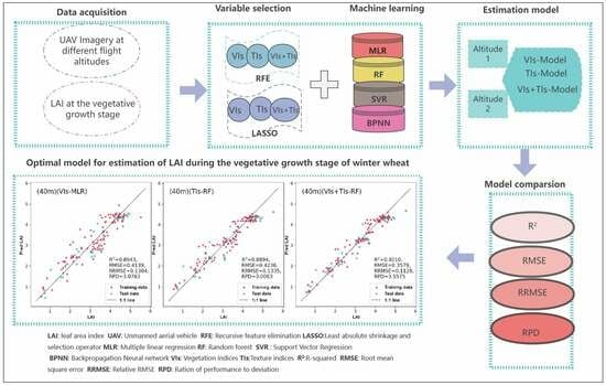
This study involved four wheat varieties, four N application rates and five N application methods in 72 plots. There are significant differences in LAI from plot to plot, and there is a complex relationship between LAI and spectral variables. Therefore, this paper, based on machine learning, simultaneously considers texture variables and spectral variables. Four models were constructed under different flight heights (20 m and 40 m) and different datasets (spectral variables, texture variables, and spectral variables combined with texture variables). The results showed that the best model was obtained by using a nonlinear model after adding texture variables (RFECV-RF, R² = 0.9210, RMSE = 0.3579, RRMSE = 0.1128, RPD = 3.5575). According to the research of Viscarra Rossel et al. [66], Lasso-RF (RPD = 3.5575) achieved an accurate estimation of wheat LAI. Although this study involved multiple wheat varieties and nitrogen application levels and methods, RFECV-RF based on texture and spectral variables can achieve high accuracy in LAI estimation.

This study provides enough spectral and texture variables for feature screening, while previous studies often artificially select a limited number of spectral variables, and the Pearson correlation coefficients between the quantitative spectral variables and the agronomic parameters are simply calculated in the study to determine the correlation of the variables to the parameters. It can be affirmed that when the relationship between the agronomic parameters and the spectral variables is linear, this practice can construct the model with excellent performance. However, when the relationship between agronomic parameters and spectral variables is nonlinear, then the accuracy when constructing the model will be limited. In this study, a comparison of different feature screening methods was conducted while providing a rich set of variables, so that RFECV-RF achieved an excellent performance.

In addition, this study was conducted during the vegetative growth stages of wheat (green-up stage and jointing stage). Unlike models established in single growth stages in previous studies, models spanning multiple growth stages have higher practicality in agricultural production, as they can more accurately predict the overall trend and changes in wheat LAI values while saving time and resources in production.

4.2. Model Comparison

This article presents the final results of using four machine learning algorithms to build models (considering two flight altitudes, three variable dataset inputs, and two variable selection methods). The results show a certain regularity; that is, in the comparison of models under different flight altitudes and different selection methods, RF or MLR becomes the most accurate model in most cases, while SVM and BPNN are not as outstanding as RF and MLR.

BPNN usually consists of an input layer, a hidden layer and an output layer. Each layer that makes up a BPNN contains multiple neurons. The different layers of a BPNN are connected to each other by weighting parameters. Thus, the complexity and performance of a BPNN depends on the number of neurons and layers, and how the weighting parameters are tuned. When the dataset is large, BPNN can adjust its parameters to better capture complex patterns and features in the input data. In this study, the reason BPNN performs worse than simple multiple linear regression may be that when the dataset is small, the parameters cannot be adjusted to the optimal values, leading to overfitting and an inability to improve the model’s generalization ability. In comparison, multiple linear regression has stronger robustness.

The MLR model improves the number of input variables based on simple linear regression, but if all VIs or TIs are used as input variables, this may lead to overfitting problems due to the complex model structure. To avoid this problem, this article conducts feature selection based on previous research. The selected variables greatly reduce the risk of model overfitting while retaining the advantages of linear models. The established linear model has strong interpretability, high computational efficiency, and wide applicability. However, MLR also has limitations and cannot capture nonlinear relationships.

The RF model achieves the best prediction results with the minimum RMSE value among all input processing, which is consistent with the research by Tang et al. [67]. RF is a powerful machine learning algorithm formed by integrating decision trees. Decision trees divide data at nodes in a nonlinear way, which means that RF can capture complex nonlinear relationships between input features. RF uses bootstrap sampling to extract multiple subsets from the original samples, constructs independent decision trees for each subset, and then combines the prediction results from multiple decision trees, overcoming overfitting problems while dealing with outliers or noise. Previous studies have also shown that RF models tend to achieve high accuracy due to their stability and robustness in handling large amounts of data.

4.3. The Combination of Vegetation Indices and Texture Information for Crop LAI Estimation

The spectral reflection characteristics provide the basis for monitoring crops. This study analyzed the applicability of 40 common spectral variables in constructing an LAI estimation model for winter wheat. After LASSO and RRECV feature selection, the predictive models have high accuracy, which validates the research results of Liu et al. [68] and Fu et al. [69]. Texture can be obtained from multispectral images and serves as a key spatial feature, containing information about the canopy surface for crop phenotype studies. Therefore, texture information has been increasingly selected in research (Li et al. [70]; Lu et al. [14]; Sarker and Nichol [71]). Hlatshwayo et al. [29] found that the texture of the red and near-infrared bands is more significantly related to LAI than some vegetation indices. Pu and Cheng et al. [16] found that texture-based features extracted from the same WorldView-2 data have a better ability to estimate and map forest LAI compared to spectral-based features.

For winter wheat LAI, we also constructed machine-learning models based on 40 texture features. The results showed that the accuracy of the texture model is lower than that of vegetation indices. Additionally, the number of texture features is greater than that of vegetation indices under different flight heights and feature selections. Vegetation indices are often combinations of multiple bands, while texture features are pixel statistics in a single band, which limits their predictive ability for vegetation parameters. Observations of the selected vegetation indices reveal that most of them are correlated with the NIR band, which has been shown to be effective in responding to the dynamics of LAI [11]. Examples include NDREI, which analyzes the red and near-infrared bands and correlates with changes in chlorophyll content, leaf area, and background soil. MSR reduces observational noise by analyzing both the near-infrared and green light bands. These reasons may lead to a better predictive performance of vegetation indices compared to texture indices alone. Texture analysis, which extracts color-independent spatial information, helps to identify objects or regions of interest in an image. The selection of appropriate bands and texture information is critical for crop LAI monitoring. Previous studies have shown that combining texture indices and vegetation indices can improve performance. Zheng et al. [18] reported that combining vegetation indices and texture improved the accuracy of rice biomass estimation. Hlatshwayo et al. [29] combined vegetation indices (VI), color indices (CI), and texture indices (TI) using the random forest (RF) method to improve the estimation accuracy of LAI and leaf dry mass (LDM). The results of this study also confirm this point. The best model based on texture variables, the RFECV-RF model (R² = 0.8894, RMSE = 0.4236, RRMSE = 0.1335, RPD = 3.0063), has significantly lower accuracy than the RFECV-RF model combining vegetation and texture indices (R² = 0.9210, RMSE = 0.3579, RRMSE = 0.1128, RPD = 3.5575).

4.4. The Impact of Different Flight Heights on Winter Wheat LAI Prediction

Previous studies have often neglected the effects of different flight altitudes when predicting LAI. To investigate the accuracy of winter wheat LAI estimation based on multispectral UAV models in response to different spatial resolutions, different flight altitudes of 20 m (resolution of 1.06 cm) and 40 m (resolution of 2.12 cm) were used in this study. Despite the twofold difference in spatial resolutions at various flight altitudes, the results of winter wheat LAI estimation indicated no significant difference in the accuracy of the model when predicting LAI at 20 m and 40 m flight altitudes. This suggests that the resolution of the image and the accuracy of the model are not proportional when making winter wheat LAI predictions, a finding that is consistent with that of Broge et al. [45]. Zhang et al. [72] also considered the scale effect of calculating vegetation indices and texture indices, and their impact on the estimation of wheat growth parameters (LAI and LDM) using machine learning algorithms. They extracted textures from unmanned aerial images at different heights during the wheat jointing stage, with pixel resolutions of 8 cm (80 m height), 10 cm (100 m), 12 cm (120 m), 15 cm (150 m), and 18 cm (180 m). The results showed that the texture at 80 m height was highly correlated with LAI and LDM, and the correlation remained generally stable at heights of 100 m, 120 m, and 150 m, despite some minor fluctuations. However, the correlation significantly decreased at a height of 180 m. This may be because when the pixel resolution is reduced to a certain extent, there are too many mixed pixels, making it difficult to distinguish between soil and vegetation, resulting in poor performance in crop growth monitoring. Although this study only explored flight heights of 20 m and 40 m, the research results on flight heights have important guiding significance for practical production. For example, the DJI P4M drone used in this study required 45 min to cover the entire study area (0.3 ha) at a height of 20 m, and the battery needing changing halfway. However, at a flight height of 40 m, it only took 15 min to cover the entire study area without the need to change the battery. In addition, not only can long flights deplete the battery, but the drone may also capture photos under different lighting conditions (caused by changes in solar zenith angle and cloud movement). This leads to uneven lighting between images, which affects subsequent data analysis and processing, ultimately affecting the prediction of LAI [73].

4.5. Limiting Factors and Future Research Prospects

When collecting multispectral images, the choices of UAV flight altitude were 20 and 40 m. Higher flight altitudes will be explored in the future to further study the effect of the spatial resolution of UAV multispectral images on the remote sensing monitoring of winter wheat LAI.

Furthermore, this study utilized data from four different winter wheat varieties at the vegetative growth stages (green-up and jointing stages) and 72 experimental plots. Future research can collect data from a broader range of winter wheat varieties across multiple growth stages, employing larger datasets, and establishing models that cover the entire growth cycle. This approach will better accommodate various growth stages, and enhance model applicability and reliability.

5. Conclusions

In this study, the feasibility of predicting winter wheat LAI based on three scenarios, namely, the vegetation index, texture index, and the combination of vegetation index and texture index, was investigated at different flight altitudes (20 m and 40 m) during the vegetative growth stages (green-up and jointing stages) of winter wheat. The results showed that a combination of different feature screening methods and machine learning algorithms can be constructed to estimate winter wheat LAI with high accuracy. The model accuracy of the combination of texture index and vegetation index was higher than that of the vegetation index model alone and the texture index model alone.

In this study, it was found that accurate models for winter wheat estimation could be established at both 20 m and 40 m flight altitudes. Therefore, in practice, we could choose a flight altitude of 40 m. This reduces the flight time relative to the 20 m flight altitude, which results in fewer battery changes and improved image quality.

In this study, a high-accuracy model for estimating the LAI of winter wheat was established by optimizing the UAV flight strategy, as well as combining the multi-feature selection method and machine learning algorithm. The model is applicable to the key stage phases of winter wheat vegetative growth (green-up and jointing stages), as well as to multiple winter wheat varieties, with high generalizability and practicality.

With different datasets, screening methods, and flight altitudes, the prediction accuracy of the RF model was almost always higher than that of the other machine learning algorithms when looking at the four machine learning methods (MLR, RF, SVM, BP) used in this study. However, further enhancement of the database and improvements in the quality of the model are needed to accurately capture the growth metrics of different crops on large-scale agricultural fields and improve the generalizability of the study results across geographic regions and crops.