
Development of a Spectral Index for the Detection of Yellow-Flowering Vegetation
by
Congying Shao
1, 
Yanmin Shuai
2,3,4,*,
Hao Wu
5,
Xiaolian Deng
6,
Xuecong Zhang
7 and
Aigong Xu
1 1
School of Geomatics and Geography, Liaoning Technical University, Fuxin 123000, China
2
College of Geography and Environmental Sciences, Zhejiang Normal University, Jinhua 321004, China
3
Xinjiang Institute of Ecology and Geography, Chinese Academy of Sciences, Urumqi 830011, China
4
CAS Research Center for Ecology and Environment of Central Asia, Urumqi 830011, China
5
Su Zhou Argo Space Technology Co., Ltd., Suzhou 215000, China
6
College of Computer and Information Technology, China Three Gorges University, Yichang 443002, China
7
School of Software, Liaoning Technical University, Huludao 125000, China
*
Author to whom correspondence should be addressed.
Remote Sens. 2023, 15(7), 1725; https://doi.org/10.3390/rs15071725
Submission received: 29 January 2023
/
Revised: 13 March 2023
/
Accepted: 19 March 2023
/
Published: 23 March 2023
(This article belongs to the Section Remote Sensing in Agriculture and Vegetation)
Abstract
:Floral phenology as a special indicator of climate change and vegetation dynamics is drawing more attention. The long-term observations of flowering events collected at scattered ground sites have accumulated valuable priority on the understanding of floral phenology, but with insufficient investigation on the spatio-temporal dynamics at regional scale, which is mainly induced by the lack of effective ways to capture the pixel-based flower events from remote sensing images. The existing yellowness indices are constructed for rape (Brassica napus L.) with less suppression to the bright background and dark green vegetation, and further with inadequate consideration on physiological characteristics and the temporal spectral signature of investigated vegetation. In this paper, we examined rape and several other representative vegetation types to determine spectral features of yellow-flower period within the growing season, then selected the visible and near-infrared bands to construct a Novel Yellowness Index (NYI) with an enhancement on the physiological mechanism of plants. The proposed NYI were discussed on the variation of mathematical properties with representative instances, cross-compared with three typical yellowness indices—Ratio Yellowness Index (RYI), Normalized Difference Yellowness Index (NDYI), and Ashourloo Canola Index (ACI) —over various yellow-flowering vegetation species at multiple scales, and validated with ground observations of three available PhenoCam network stations and field phenological observations at Görlitz, Sachsen, and Germany. In addition, we applied NYI to detect the rape field using Sentinel-2 image at Görlitz with typical rape area as a case study. Results show that the proposed NYI exhibits the potential to capture yellow-flowering events with increased sensitivity to the variation of flower density, and reduction of noise introduced by bright background or dark green vegetation of multiple vegetation species at different scales. As the flower density increases from 33% to 78%, the relative differences of NYI captured can reach up to 74%, compared with other three indices which have the relative differences no more than 57%. The cross-comparison indicates NYI performs better with higher consistent with PhenoCam observation and Deutscher Wetterdienst phenological station than other yellowness indices in capturing the variation of yellow flower density. The case study of NYI application in the identification of rape field exhibits good accuracy with the overall accuracy up to 97.5%, the Kappa coefficient of 0.94, and F score of 0.96. Consequently, the satellite-derived yellowness index will be a potential means to investigate the flowering dynamics and planting range of yellow-flowering vegetation such as rape.

1. Introduction
The dynamic of vegetation phenology is an important indicator of climate change and even global environmental change [1,2]. Numerous studies of vegetation phenology have been focusing on the dynamic of photosynthetic activities, identification of phenology phases, such as green-up, maturity, senescence, and dormancy, from satellite-based vegetation indices [3,4]. Flowering as an important phenology event within the life cycle of plant, may alter processes at species, communities, and ecosystem levels. Related phenology studies have indicated that flowering can affect the frequency of plant–herbivore and plant–pollinator interactions as well as the effectiveness of plant pollination [5,6,7]. The long-term investigation indicates a mismatch in phenology between plants and pollinators may contribute to local species extinction [8]. Moreover, flowering is also an essential determinant of yield for many crops in agricultural systems [9,10,11]. Regional observation-based studies have demonstrated that warmer temperatures and earlier flowering can shorten crop development stages, which may reduce agricultural yields [12]. Therefore, it is vital to timely acquire and accurate spatio-temporal information on the flowering of vegetation.
Phenological observations of the ground have contributed to understanding the changes in vegetative and floral phenology in response to climate change. However, traditional observation methods are usually time-consuming and labor-intensive to cover many species across a region and establish long-term data records, as well as being difficult to apply across space and time and unable to capture important spatial and temporal variations [13]. The development of remote sensing technology and the opening and accumulation of satellite data provide objective guarantees for acquiring spatial and temporal details of vegetation phenology. Through monitoring the phenology of winter wheat in Yucheng, Shandong, China, an almond orchard in California, and a deciduous forest in Bartlett, New Hampshire, USA, Shuai et al. found that MCD43A4 data can capture not only phenological events (e.g., flowering) but also substantial interannual variability compared with ground records [14]. Related studies indicated that remote sensing is always adopted to investigate phenology efficiently and economically, focusing on phenological events such as green-up, maturity, senescence, and dormancy [3,4,15]. Some pioneering studies have attempted to explore the possibilities of remote sensing in quantifying flowering status, such as Chen’s analysis of multi-scale remote sensing observations demonstrating that an enhanced bloom index can quantify the flowering status of almond orchards in California [16].
Although there are relatively few studies on floral phenology, some studies have attempted to monitor the flowering of yellow-flowering vegetation (e.g., rape) using remote sensing. Based on the characteristic that green and blue bands are strongly correlated with the flower density of rape, a few related indices are constructed for the identification of the rape flowering stage [17,18,19,20]. Although these indices are capable of identifying the flowering phase, they lack in-depth analysis between the spectral characteristics of rape and other crops during the growing season. Additionally, these indices show low sensitivity when it comes to distinguishing dark green vegetation from rape. On this basis, a few researchers pointed out that the rape can be distinguished from other vegetations by analyzing the spectral difference between rape and other crops during the growing season and then choosing the most suitable one from a series of combined indices based on the selected spectrum [21,22]. However, this method ignores the specific physiological characteristics of rape and only focuses on the difference between rape and other vegetations which could limit the application of these indices to other yellow-flowering vegetations, for example, royal chrysanthemum and sunflowers. In addition to the influence of other crops, the side effect of high brightness features is inevitable during the growing season. Ignoring the impact of high-brightness features can affect the accuracy of identifying the flowering stages of rape as well. These studies have shown that information on the flowering of rape can be obtained successfully by remote sensing. However, several challenges still persist. On one hand, they tend to focus solely on rape and exhibit low sensitivity to distinguishing yellow flowers from bright features, dark green vegetation, and dark green pods. On the other hand, these indices primarily concentrate on time-series spectral features and do not comprehensively leverage spectral and physiological characteristics to develop a yellowness index.
Thus, a new spectral index NYI (Novel Yellowness Index) is proposed in this paper. This index takes into account the physiological characteristics of yellow-flowering vegetation and their relationship with spectral characteristics. It also mitigates the influence of dark green vegetation and dark green pods, thereby highlighting the characteristics of yellow-flowering vegetation. To validate the feasibility of our proposed index, the proposed index is first compared with the other three indices from the aspects of different observation scales, different yellow-flowering vegetation species, and different flower densities and phenological observations, and then applied to a selected area in Görlitz, Sachsen, Germany. In the following, the introduction of the data is described in Section 2. The New Yellow Index and its related properties are proposed in Section 3. The results and discussion are analyzed in Section 4. The conclusions are presented in Section 5.
2. Data
Based on the research requirements of surface cover characteristics, scale size, and the current spatial and temporal resolution, data openness, sensor band settings, and data product quality of remote sensing images, two different observational scales of multispectral images, Landsat 8 (L8), Sentinel-2, and MCD43A4, were selected. The Deutscher Wetterdienst (DWD) phenological observation network and PhenoCam Network were also selected to determine the flowering and compare the differences of different yellowness indices. In addition, to explore the performance of the NYI on identifying rape, EUCROPMAP 2018 and RapeseedMap10 were selected for comparison and verification.
2.1. Surface Reflectance Data
This study employed Landsat 8, Sentinel-2, and MCD43A4 provided by the United States Geological Survey (USGS), European Space Agency (ESA), and NASA at the Google Earth Engine (GEE) cloud platform. Landsat 8 has a spatial resolution of 30 m in the eight multispectral bands. In comparison, Sentinel-2 is equipped with a multispectral instrument with thirteen spectral bands, with a spatial resolution of 10 m in the visible and near-infrared, and 20 m in the four red edges and two shortwave infrareds. The surface reflectance (SR) of L8 and S2 archived in the GEE are radiometric and geometric correction and atmospheric correction, with an accuracy of geometric correction better than 0.5 pixels [23,24]. MCD43A4, the Nadir Bidirectional Reflectance Distribution Function (BRDF)-Adjusted Reflectance (NBAR) dataset, has a spatial resolution of 500 m in the seven multispectral bands and removes the view angle effects. The GEE addresses for L8, S2 and MCD43A4 are “LANDSAT/LC08/C02/T1_L2”, “COPERNICUS/S2_SR”, and “MODIS/006/MCD43A4”, respectively. We adopted Landsat 8 SR from 2020 to 2021, Sentinel-2 SR from 2019 to 2021, and MCD43A4 from 2005 to 2018 using quality control to remove clouds and cloud shadows, and resampling the red edge and shortwave infrared of Sentinel-2 to 10 m.
2.2. Crop Products
2.2.1. EUCROPMAP 2018
The EUCROPMAP (European Union Crop type Map) was produced by the European Union, Joint Research Centre, and is currently only available for 2018. Capitalizing on the unique LUCAS 2018 Copernicus in situ survey, this dataset is the first continental crop-type map with a 10 m pixel size for the European Union based on S1A and S1B Synthetic Aperture Radar observations for the year 2018. The Random Forest algorithm detected 19 different crop types, including common wheat, durum wheat, barley, rye, oats, maize, rice, sugar beet, sunflower, rape, and soya, etc. The coefficient of determination (R2) between the remotely sensed estimated and the Eurostat-reported rape area is 0.97. User accuracy and producer accuracy for rape in Germany are better than 97%, with an F score of 0.90 [25]. This paper adopted the EUCROPMAP to obtain spatial distribution for rape in 2018.
2.2.2. RapeseedMap10
The RapeseedMap10, 10 m rapeseed planting areas in 33 European and American countries in 2017–2019, was produced by the Food Security Research and Education Team of Beijing Normal University based on the growth phenology and spectral and polarization characteristics of rape, combined with Sentinel-2, Sentinel-1, and other multi-source data. The coefficient of determination (R2) between the estimated area of rape and the FAO reported area is 0.88, with a user accuracy of 95%, producer accuracy of 88%, and an F-score of 0.91 for Europe [26]. The 10 m rape distribution map for 2018 was selected for this paper.
2.3. Ground Phenological Observations
The Deutscher Wetterdienst (DWD) phenological observation network traced back to 1882 is operated by Germany’s national meteorological service. At present, about 1200 observers participate in this network, most of them on a voluntary basis. Approximately 160 phenological phases of wild plants, agricultural crops, fruit trees and bushes, and grapevines are observed and archived in the phenological database of the DWD (http://www.dwd.de/phaenologie, accessed on 20 May 2022). Each DWD record is considered to represent the crop phenology within a maximum distance of 5 km from its location. The basic information for each station includes the following: station name, location, vegetation type, vegetation phenological phase, and quality control [27], and where the crop phenology was recorded in the field following the BBCH (Biologische Bundesantalt, Bundessortenamt, and Chemische Industrie) scale [28]. For rape, the beginning (i.e., BBCH61) and end (i.e., BBCH69) of the flowering dates of the DWD are available, while the peak of the flowering date (i.e., BBCH65) is not. Based on satellite images and crops within 5 km of the phenological observations, Großhennersdorf (ID: 12197), a rape observation station from 2018, was selected for this paper, and the start and end of flowering at this site can be obtained from the observation records.
The PhenoCam network was established in 2008, which served as a way of tracking vegetation phenology in a variety of ecosystems across North America and around the world by digital camera imagery, and currently includes over 700 sites. They use StarDot NetCam CS to collect RGB (red, green, blue) and IR (infrared) images every 15 min at each of its field sites, totaling more than 60 million images. The images and data are publicly available in near real time via a web page (https://phenocam.sr.unh.edu/webcam/, accessed on 20 May 2022). At terrestrial sites, the Phenocam is mounted at the top of the meteorological/flux tower (typically at 2 m) to capture above canopy vegetation information, and the camera is usually pointed north (in the northern hemisphere) to minimize lens flare, shadows, and forward scattering of the canopy, and is inclined downward at 20–40° [29]. Basic information about each site includes the following: site type, site name, location, start and end date of site images, camera description, vegetation type, climate type, etc. In this paper, cafcookeastltar01, cafcookwestltar01, and cafboydnorthltar01, three phenological sites of spring rape in 2021 provided by Cook Agronomy Farm (CAF) in Pullman, Whitman, Washington, USA, were selected for validation of the yellowness index.
In this study, we have selected seven typical areas with yellow-flowering vegetation, namely, Zhaosu County in Xinjiang, Hanzhong City in Shaanxi, Yancheng City in Jiangsu, Jingmen City in Hubei, Wuyuan County in Jiangxi, Sachsen in Germany, and Pullman in Washington, USA, as shown in Figure 1. These areas have been chosen to develop and validate the proposed yellowness index. Selected areas have different geographical locations, climates, and vegetation species. Zhaosu is the westernmost spring rape planting area in China (Figure 1A-a), with a temperate continental climate. Spring rape in this area is sown in April and flowers in July. Hanzhong is one of the traditional production bases for rape cultivation in China (Figure 1A-b) and has a northern subtropical climate. Winter rape in the region is sown in November and flowers from March to April of the following year. Yancheng is on the northern flank of the Yangtze River Delta in China (Figure 1A-c) and has a subtropical monsoon climate. Winter rape in this region is sown in November and flowers from March to April of the following year. Jingmen has one of the densest winter rape cultivations in the Yangtze River Basin in China (Figure 1A-d), with a north subtropical monsoon climate. Winter rape in this region is sown in November and flowers from March to April of the next year. Wuyuan has a subtropical monsoon humid climate. The royal chrysanthemum in this region is transplanted in April–May and flowers in November (Figure 1A-e). The German rape observation Großhennersdorf is located in Görlitz, Sachsen (Figure 1C), which has a temperate maritime climate. Winter rape in this region is sown from August to September and flowers from April to May of the following year. Three phenological stations in Pullman, Whitman, Washington, USA, are provided by CAF (Figure 1B). The farm is a long-running agroecosystem research site operated by Washington State University and follows a three-year crop rotation, with spring and winter wheat planted two out of every three years and a third crop of either spring rape, winter lentils, spring or winter peas, or spring or winter barley. Spring rape on this farm is sown in April and flowers in June.
In this paper, Sentinel-2 from Zhaosu in 2019, Hanzhong in 2021, and Yancheng in 2020 were selected to investigate the spectral characteristics of typical ground objects and develop the new yellowness index, and multispectral images from Zhaosu in 2021, Yancheng in 2020, Jingmen in 2020, Wuyuan in 2020, Sachse in 2018, and Pullman in 2021 were then adopted to evaluate the performance of the Novel Yellowness Index. Finally, Görlitz in 2018 was selected to explore the performance of the NYI with regard to identifying rape.
3. Development of Yellowness Index
In this study, measures shown in the processing chain (Figure 2) are adopted to develop a new yellowness index. The main components include development, verification, and application of the yellowness index.
3.1. Investigation of the Time-Series Spectral Characteristics for Rape and Other Crops
To capture the spectral characteristics of rape in different regions and different climates, two samples of spring rape in Zhaosu, and winter rape in Hanzhong and Yancheng were selected, respectively, and one sample of other non-yellow-flowering vegetation, including wheat, maize, soybean, and forest, was also selected to compare the temporal spectral characteristics of different vegetation types and analyze the differences in their temporal spectral characteristics based on Sentinel-2 data. Figure 3 and Figure 4 present the time series spectral characteristics for typical features based on Sentinel-2 at Zhaosu in 2019, Hanzhong in 2021, and Yancheng in 2020, respectively. During their own growth stage, typical ground objects have the spectral characteristics for typical green vegetation. However, typical ground objects have different behaviors in each band. For rape, the reflectance ranges are from 0.04 to 0.15 in the red band and from 0.06 to 0.17 in the green band, while the range is between 0 and 0.1 in the red and green bands for all other vegetation (Figure 3a,b). Rape reflects slightly more than other vegetation types in the red and green bands, with less difference in the other bands (Figure 3).
Different vegetation naturally has distinctive growth and development cycles and color changes, and their spectral reflectance characteristics are mostly distinctive in different seasons. Rape has three different canopy morphologies during the growing season, namely, the vegetative stage with a green canopy dominated by leaves, the flowering stage with a yellow canopy dominated by yellow petals, and the mature stage with a green or brown canopy due to pods and branches [19]. Compared to the non-flowering phase, both spring and winter rape have high reflectance in the green, red, and NIR bands at the flowering phase, and the reflectance in the green, red, and NIR bands increases as the rape flowers and then decreases as the flowers fall (Figure 3a,b and Figure 4). The magnitude of reflectance variation between different bands depends on the flower density. The reflectance of the green band and red band at the flowering phase can increase by 110% and 230% at most, while the increase in the NIR band is relatively small, up to 33%, compared with that before the flowering. In the case of Zhaosu, the reflectance for the green and red bands changes from 0.082 and 0.039 (day of year (DOY):175) before flowering to 0.166 and 0.129 (DOY:190) at flowering, respectively, and then declines (Figure 3a). The difference between the red and green bands became smaller when the rape is in bloom, for example, the difference between the red and green bands changes from 0.043 (DOY:175) before flowering to 0.037 (DOY:190) at flowering and then increases (Figure 3a) in Zhaosu. For rape, the most discernible spectral differences between flowering and non-flowering can be identified by the green and red bands, in agreement with previous studies [30,31,32]. As a result, the reflectance for red and green bands of rape reaches local maxima during the peak of flowering. However, during the growth period of rape, winter rape has a higher reflectance in the visible band affected by snow, even higher than that at flowering (Figure 4c,d). Other vegetation, such as wheat, shows less variation in reflectance of the green and red bands compared with rape. Therefore, the change in reflectance of the green and red bands can be employed as a distinctive spectral feature to identify rape flowering.
The spectral reflectance of the crop canopy is closely related to morphological and physiological characteristics. Leaf composition and molecular structure affect crop reflectance. Consequently, ratios or differences in different bands such as visible, NIR, and shortwave infrared can be used to characterize plants [33]. At the flowering stage of vegetation, yellow flowers appear among the green leaves, which significantly alters the optical reflectance properties of the canopy, being a combination of reflected energy from both the yellow flowers and green leaves of the vegetation [19,29]. The yellow-flowering canopies reflect more and absorb less between 500 mm and 700 nm, but reflect less and absorb slightly more than vegetative canopies between 400 mm and 500 nm [19], because the carotenoids in the petals absorb blue light, so reflect a mixture of red and green light which we perceive as yellow. For rape [32] and yellow-flowering species of buttercups [34], the green and red bands are the most distinctive spectral differences between yellow-flowering and non-yellow-flowering. In addition, the reflectance of the near-infrared band is positively correlated with flower density in rape [19,29]. Therefore, the red, green, and near-infrared bands were chosen as the appropriate bands to distinguish yellow-flowering from non-yellow-flowering, and it was considered that snow may affect the spectral reflection of winter rape (Figure 4c,d). Finally, the visible and near-infrared bands were chosen to construct a new yellowness index.
3.2. Construction of Yellowness Index
The spectral characteristics of rape indicate that the reflectance in the red, green, and NIR bands is high during flowering, with the red and green bands even reaching a local maximum at the peak of flowering. At the same time, the differences between the red and green bands become smaller. According to the special spectral characteristics of yellow-flowering vegetation, the new yellowness index is constructed by considering both the yellowness and brightness characteristics of rape at flowering, and weakening soil and snow effects. The yellowness index is expressed in Equation (1).
where represents the yellowness index, are the reflectance of red, green, blue, and NIR bands, respectively, and Sign represents the sign function. Specifically, the sum of the red-green-NIR band reflectance (i.e., Brightness) in the numerator was used to represent the overall higher reflectance of yellow flowers. In addition, the sign of the difference between the red and green bands (i.e., GVGTSignature) was added to the numerator to further identify green vegetation information because green vegetation in the green band was usually much higher than that in the red [16]. To suppress the effects of bright features such as snow, the absolute value of the difference between the red and blue bands (i.e., HighlightSuppression) is introduced as another multiplicative term in the numerator based on the difference between bright features and rape in the visible band. A function (i.e., Yellowness) with e as the base and the difference between the red and green bands as the exponent is added to the denominator to indicate the yellowness of yellow flowers based on the spectral and color characteristics of the vegetation when it has yellow flowers [35].
To better understand and apply the yellowness index, the fundamental mathematical properties of the yellowness index are analyzed in relation to the reflectance characteristic of each band. The remote sensing properties of the yellowness index are then further explored in conjunction with the spectral library provided by the spectral library of USGS and ASTER and the Chris Elvidge vegetation spectral library. Considering the mathematical and remote sensing characteristics of the yellowness index, linear transformation of the yellowness index is carried out to highlight its yellowness grade.
The basic properties of the yellowness index are first investigated. Based on the expression for the yellowness index, the boundedness of the index can be discussed in four cases, namely , , , . This paper takes as an example to examine the boundedness of the yellowness index in detail.
When , the index indicates green vegetation, as shown in Equation (2).
where represents the yellowness index, are the reflectance of red, green, blue, and NIR bands, respectively.
When , the equation is shown as Equation (3).
where and are the same as those represented in Equation (2).
Assumed that and , the partial derivative of Equation (3) is taken, with respect to is constantly less than 0. For and , the related partial derivatives are constantly greater than 0. Then the yellowness index is monotonically increasing with and decreasing with . From the monotonicity, it is clear that the maximum value is taken at , bringing to Equation (3), the partial derivative with respect to is constantly less than 0, and the maximum value cannot occur at , due to the limitation of . Therefore, Equation (3) reaches maximum value 3 when . At , the partial derivative with respect to is always greater than 0 regardless of the value of , and the minimum value is 0 at . Therefore, at , the range of f is . Similarly, the boundedness of the yellowness index in the other three cases can be easily deduced. Combining all the four cases, the range of the yellowness index is .
To further understand yellowness index function, the image method is adopted to visualize the yellowness index function, which can intuitively exhibit the boundedness and monotonicity of yellowness index. Taking as an example, Figure 5 illustrates the boundedness and monotonicity of the yellowness index function. From Figure 5a, the yellowness index is bounded by the section. If , the yellowness index increases monotonically with and decreases monotonically with . Otherwise, the yellowness index decreases monotonically with and increases monotonically with . In addition, Figure 5b takes as an example (the red rectangle in Figure 5a), and the yellowness index increases monotonically with .
According to the actual reflectance of surface features, the remote sensing characteristics of the yellowness index are explored with the open spectral library. The reflectance spectra of three typical ground objects, including soils (41), water bodies (6), and vegetation (96), were selected from the ASTER, USGS spectral library, as well as from the Chris Elvidge vegetation spectral library of ENVI (listed Table 1). Based on the reflectance spectrum of the selected ground objects, the reflectance ranges of vegetation and non-vegetation in the blue, green, red, and near-infrared bands are determined. Thus, the boundedness of the yellowness index in vegetation and non-vegetation is defined as , , respectively. In addition, the yellowness index is linearly transformed to highlight the yellowness scale, considering the mathematical and remote sensing characteristics of the index. With as the critical point for linear transformation, the main transformation region is concentrated in , and the other regions are not linearly transformed, as shown in Equation (4).
3.3. Yellowness Index of Typical Ground Objects
To better elucidate our proposed NYI, the yellowness index of typical ground objects was calculated using Sentinel-2 and MCD43A4 data by Equation (1), and characteristics of the yellowness index between different vegetations were compared to analyze the characteristics of their time series. In addition to the samples for constructing the yellowness index in Section 3.1, an additional 4280 samples of different vegetation in Northeast China were used to illustrate the yellowness index for typical ground objects. These samples consisted of 18.8% soybeans, 1.5% wheat, 48.3% maize, 22.1% paddy, and 4.7% forest and grassland. Figure 6 and Figure 7 present the time-series characteristics of the yellowness indices for typical ground objects based on Sentinel-2 and MCD43A4, including spring rape, winter rape, sunflower, wheat, maize, soybean, paddy, forest, and grassland, respectively. As can be seen from Figure 6, the yellowness index in all three regions has a clear peak at the flowering stage of rape, up to ~0.7, which is much higher than other stages of the growth period. For example, the yellowness index is around 0.1 at the seedling and bud stage of rape and 0.2 at the pod development and maturity stage as the mature pod color is close to yellow. The magnitude of the yellowness index increases with the increase in different degrees of flowering, i.e., flower density, for example, in sample 1 can reach 0.64 on Julian day 190 of flowering, while sample point 2 is only 0.26 on Julian day 205 of flowering in the Zhaosu. As can be seen from Figure 3(a2,b2), the rape flowers in sample 1 are more yellow than those in sample 2. Another type of yellow-flowered vegetation, the sunflower, exhibits a peak in the yellowness index throughout all stages of its flowering, with values reaching up to about 0.3. This is considerably higher compared to other stages of the growing season. In addition, during the growth period of other non-yellow-flowering vegetation, the yellowness index fluctuates slightly, around 0.1, with soybean and paddy. At their maturity, the corresponding yellowness index has a minor rise, at around 0.2, due to their color approaching yellow (Figure 6 and Figure 7). Consequently, the NYI can capture the flowering period of rape and monitor its flower density.
4. Results and Discussion
Three existing yellowness indices were selected to verify the NYI constructed in this paper, namely, the RYI [17], NDYI [18], and ACI [21]. The following comparison is mainly carried out from different observation scales, different yellow-flowering vegetation species, different flower densities, and ground phenological observations.
The variation of different flowering stages was evaluated by measuring the relative difference (RD) in yellowness indices at different flowering stages. The greater the variation in a given yellowness index between different stages during flowering, the more influentially the yellowness index reflects the various stages of plant flowering. The variability of the yellowness index is shown in Equation (8).
where and represent the yellowness indices for two different flowering stages, respectively.
To determine what stage of flowering is currently used to calculate the yellowness index, the bloom coverage (BC) is calculated by Equation (9) using the higher resolution image as a reference.
where is the number of pixels at the flowering stage in the higher resolution image corresponding to the selected pixel, and is the total number of pixels in the higher resolution image corresponding to the selected pixel. Taking the 30 m Landsat as an example, some sample points were selected to characterize the flowering stage of the vegetation, and the yellowness index was calculated. This is then referenced to a 10 m resolution Sentinel-2 high-resolution image, where is nine and is the number of pixels in the flowering stage in nine pixels.
4.1. Comparison of Different Observation Scales
To verify the feasibility of the proposed NYI under different observation scales, Landsat 8 and Sentinel-2 data were selected to compute different yellowness indices by Equations (1) and (5)–(7), including the RYI, NDYI, and ACI of spring rape in Zhaosu. The proposed indices were compared with the existing ones, and the differences of their time series characteristics were analyzed. Figure 8 and Figure 9, respectively, exhibit a comparison of the four yellowness indices for Sentinel-2 and Landsat 8 in Zhaosu in 2021. A visual interpretation of the true color composite of these imageries in Figure 8 and Figure 9 reveals the temporal dynamics of bloom in spring rape. As can be seen from the true color composite images of Sentinel-2 in Figure 8, no flower signals of spring rape are observed until 3 July (Figure 8a,b). Spring rape blossoms on 18 July (Figure 8c), remains in flower on 23 July (Figure 8d), and is out of flowering on August 2 (Figure 8e). A similar flowering dynamic is observed from the corresponding NYI imagery (Figure 8u–y). The NYI exhibits a low value before 3 July, a rapid increase on 18 July and 23 July, and a decrease on August 2. Note that the yellowness index differs between 18 July and 23 July for flower density of spring rape (Figure A1m–o). The magnitude of the NYI rises with increasing flower density. Similar spatial and temporal patterns exist in the Landsat imagery, as well as the derived yellowness index imagery (Figure 9). Consequently, the constructed NYI can capture the flowering period of spring rape and distinguish flower density at different observation scales of Sentinel-2 and Landsat 8. Although the existing yellowness indices, including the RYI, NDYI, and ACI have the ability to recognize the flowering period of spring rape, they have some defects under some specific situations. The RYI and NDYI have high values in the non-flowering period of rape and green vegetation, even higher than the flowering period of rape, which fails in highlighting the different flowering degrees of rape. The ACI in the highlighted built-up areas shows a comparable value to the flowering stage of rape, which may cause improper recognition, but the effect of highlighting the flower density of rape is not obvious. In contrast, our proposed NYI not only captures the flowering period of rape, but also effectively avoids the shortcomings mentioned earlier, and obviously highlights the flowering density of rape.
To detect more detailed dynamics of the bloom status, a sample was selected to monitor the whole growth period of rape. Figure 10 shows the temporal characteristics of the different yellowness indices of rape at the different observation scales of Sentinel-2 and Landsat 8. Our proposed NYI can capture the flowering stage of rape, and both have apparent peaks at the flowering stage, up to ~0.8, which is much higher than other stages in the growth period (Figure 10). The NYI is around 0 at the seedling and bud stage of rape, and has a slight increase to ~0.3 at the pod turning yellow during pod development and maturity stage. The RYI and NDYI also fluctuate considerably during the non-flowering phase. However, the RYI and NDYI continue to show high values at the development and maturity stages of the pod, even higher than during the flowering phase. Whereas ACI fluctuates slightly during the non-flowering phase, the difference between the flowering and non-flowering phases is slight and hardly distinguishable. For the flower density of rape, the RYI and NDYI cannot distinguish flower density, the ACI can slightly distinguish, while the yellowness index constructed in this paper can highlight the flower density of rape. For example, the true color composite image of Sentinel-2 is more yellow on 23 July than on 18 July. The RYI and NDYI are basically unchanged, but the yellowness index constructed in this paper changed from 0.66 on 18 July to 0.77 on 23 July, reflecting the yellowness level, and the ACI increased slightly from 0.21 on 18 July to 0.22 on 23 July. Therefore, our constructed NYI can successfully distinguish the flowering period from the growth period.
4.2. Comparison of Different Species of Yellow-Flowering Vegetation
The Sentinel-2 data were used to calculate different yellowness indices of winter rape in Yancheng and Jingmen and royal chrysanthemum in Wuyuan using Equations (1) and (5)–(7) to verify the applicability of the constructed NYI under different climate and yellow-flowered vegetation species. We compared the indexes proposed with the existing yellowness indexes to analyze the differences in their time-series characteristics. Figure 11, Figure 12, and Figure 13, respectively, display the comparison of the four yellowness indices for winter rape in Yancheng and Jingmen and royal chrysanthemum of Sentinel-2 in Wuyuan in 2020. The true-color composite images in Figure 11, Figure 12, and Figure 13 reveal the flowering dynamics of winter rape and royal chrysanthemum, respectively. As shown in Figure 13, the true-color composite image reveals that no flower signal of royal chrysanthemum is captured until October 23 (Figure 13a,b). It is in flowering on November 7 (Figure 13c), and November 12 (Figure 13d) and generally over on December 22 (Figure 13e). The corresponding NYI images show similar flowering dynamics (Figure 13u–y). The sentinel-2 images and corresponding yellowness index images of Yancheng and Jingmen exhibit similar spatial and temporal distribution characteristics (Figure 11, Figure 12 and Figure A3). Compared with the recognition of royal chrysanthemums, the three yellowness indices (RYI, NDYI, and ACI) perform better in identifying the flowering stage of winter rape, while the RYI and NDYI have poor recognition in the flowering stage of royal chrysanthemum, with some omission identifications. As mentioned previously in Section 4.1, the disadvantages of existing indices are that the RYI and NDYI have high values in green vegetation and the non-flowering stage of yellow flowers is more apparent in royal chrysanthemum.
Figure 14, Figure 15 and Figure 16 show the temporal characteristics of different yellowness indices under different yellow-flowering vegetation species of winter rape and royal chrysanthemum. The NYI constructed in this paper of both rape and royal chrysanthemum has significant peaks at each flowering stage, up to approximately 1, much higher than at other stages of the growth period. During the seedling and bud stage of rape, the NYI generally ranges from 0 to 0.1, with a slight increase of about 0.2 as the pods turn yellow during the development and maturity stage of the pod. The RYI and NDYI also fluctuate considerably during the non-flowering phase. For example, the RYI and NDYI still have high values at the development and maturity stage of the pod. The ACI fluctuates slightly during the non-flowering period, but the ACI in winter rape has high values during the non-flowering period at Yancheng on February 16 (DOY:47) disturbed by snow (Figure 14). There is a slight difference between the flowering stage and non-flowering stage of the ACI, especially for royal chrysanthemum, where the flowering stage and non-flowering stage are nearly identical. Note that the Sentinel-2 true color composite image of royal chrysanthemum is more yellow on November 7 than on November 12, Figure 13, which can be captured obviously by the NYI. Compared with the index value on November 7, the constructed NYI decreased by 47%, while the other indices decreased by less than 19%. Therefore, our proposed index can not only capture the flowering stage correctly, but also shows higher superiority in distinguishing flower density and avoiding interference from green vegetation and highlighted features.
4.3. Comparison of Different Flower Densities
Although the above results of Section 4.1 and Section 4.2 qualitatively exhibit the performance of different yellowness indices at different flower densities, and experiments show that the NYI has a significant advantage in highlighting the flower density compared to existing yellowness indices, quantitative information is required to evaluate the degree of differentiae. Therefore, this section compares the differences between the different yellowness indices from a quantitative perspective. The different yellowness indices of rape were first calculated using Landsat 8 data from Jingmen on 19 March 2020 through Equations (1) and (5)–(7), followed by the calculation of coverage according to Equation (9) using Sentinel-2 on 18 March 2020 as a reference. Figure 17 shows the different flowering coverage of rape in Landsat 8 corresponding to Sentinel-2 as a reference image. A total of 12 samples at 33.33%, 77.78%, and 100% of flowering coverage were selected to evaluate the performance of different yellowness indices at different flowering densities. Figure 18 illustrates the relative differences between these coverages for the RYI, NDYI, ACI, and NYI. The relative differences of the RYI, NDYI, ACI, and NYI are 13%, 17%, 57%, and 74%, respectively, when rape flowering coverages change from 33.33% to 77.78%. In contrast, the relative differences in the RYI, NDYI, ACI, and NYI are 20%, 21%, 29%, and 46%, respectively, when coverages change from 77.78% to 100%. The RYI and NDYI are more consistent in distinguishing between rape flowering coverages, with slight relative differences during the change in coverage from 33.33% to 100%, and a negative correlation between the increase in relative differences and the increase in coverage, while the ACI and NYI have significant relative differences and a positive correlation between the increase in relative differences and the increase in coverage. In addition, the most remarkable relative differences in the NYI are observed with changes in coverage.
4.4. Comparison with Ground Phenological Observations
Ground phenological observations were adopted as the third party to further evaluate the performance of the proposed NYI and the three existing indices. Based on Sentinel-2 data, the different yellowness indices for winter rape in Sachsen, Germany, and spring rape at Cook Agronomy Farm in Pullman, Washington, USA, were calculated by Equations (1) and (5)–(7) to compare the difference between the proposed indices and the existing yellowness indices in terms of temporal characteristics based on ground phenological observations.
The phenological observation network of Germany can obtain the start and end of flowering at the stations from the observation records to verify the accuracy of the constructed NYI. Based on satellite images and crop situation within 5 km of the phenological observation, the winter rape observation station—Großhennersdorf in 2018—was selected for this paper and the flowering period of the site was obtained from the observation records. Figure 19 shows a comparison of the four yellowness indices for winter rape of Sentinel-2 in the 5 km surrounding the phenological site Großhennersdorf. This site provided a phenological record of the flowering phase from 21 April to 17 May (DOY:111-137), representing winter rape phenology within 5 km of the site. Flowering dynamics of winter rape are revealed by the true color composite image of Sentinel-2 in Figure 19a–e, which is consistent with the flowering period recorded by the phenological observation. The corresponding NYI exhibits similar flowering dynamics (Figure 19u–y), that is, the NYI is low until 21 April, but increases rapidly on 4 May and 6 May, still increases on 14 May in some areas, and decreases on 21 May, while the NYI is different between 4 May, 6 May, and 14 May due to different density of winter rape, and the yellowness index is positively correlated with flower density of winter rape (Figure A5m–o). Moreover, the ACI has high values in highlighted bare land and highlights the rape flower density. Similar performances of the RYI, NDYI, ACI, and the yellowness indices in the recognition of rape are also observed here, as mentioned previously in Section 4.1.
To capture more detailed flowering dynamics, a sample was selected to monitor the whole growth period of winter rape, and Figure 20 illustrates the temporal characteristics of different yellowness indices for winter rape based on Sentinel-2. Compared with ground phenological observations, the proposed NYI can capture the flowering stage of rape, with a clear difference between the flowering phase and non-flowering phase (with a significant peak at the flowering stage of rape.), while the ACI fluctuates during the non-flowering phase, such as after the winter rape harvest comparable to the ACI during the flowering phase of rape. The RYI, NDYI, ACI, and the constructed NYI can all highlight the flower density, but the degree of highlighting is dissimilar. For example, the true color composite image of Sentinel-2 is more yellow on 6 May than on 4 May. The RYI, NDYI, ACI, and NYI change from 2.85, 0.48, 0.21, and 0.82 on 4 May to 3.07, 0.51, 0.24, and 0.99 on 6 May, respectively. The increase in magnitude of the RYI, NDYI, and ACI is basically the same, while the increase in the index constructed in this paper is higher than the existing three indices. Thus, the proposed NYI captures the flowering period of rape, is consistent with ground phenological observations, avoids interference from green vegetation and highlighted features, and highlights the flowering density of rape.
The accuracy of the NYI can be further verified by the real-time crop photos provided by the Phenological Camera observation network in the United States. In this paper, three phenological sites (cafcookeastltar01, cafcookwestltar01, and cafboydnorthltar01) of spring rape in 2021 were selected to verify the yellowness index. Figure 21 exhibits the temporal characteristics of the different yellowness indices for winter rape in 2021 at three phenological stations, respectively. As can be seen from Figure 21, the maximum of the proposed NYI of winter rape is around 0.60 during the flowering stage and 0.2 during development and maturity of the pod. Similar to the above analysis, the RYI and NDYI generally capture the flowering period of winter rape except for the development and maturity of the pod and the period after the harvest for the rape, while the ACI performed poorly in capturing the flowering stage of winter rape, with no significant peaks during the flowering stage and continued to have high values even above flowering after the mature harvest. Notably, the performance of the RYI, NDYI, and ACI is slightly weak in capturing the flowering at the cafcookwestltar01 due to the mix of bare soil and winter rape at this site, resulting in lower flower density. At the same time, the different yellowness indices vary with the flower density. Based on the photos of winter rape captured by the phenology camera, the yellowness of rape shows an “inverted V”, that is, the yellowness increases first, reaches a peak, and then decreases. Figure 21 exhibits that only the proposed NYI presents an “inverted V” during the flowering period of winter rape, which can better capture the different flower densities, while the RYI, NDYI, and ACI perform poorly in distinguishing flower density, especially the ACI. The superiority of our proposed index is confirmed by ground phenological observations.
In summary, the index can capture the flowering period and highlight the flower density at different observation scales of Sentinel-2 and Landsat 8, and different yellow-flowering vegetation species consisting of spring and winter rape and royal chrysanthemum. Compared with ground phenological observations, the index can also capture the flowering period of rape more accurately, and is consistent with the ground observation.
The shortcomings of currently available yellowness indices are attributed to the bands chosen for their construction. The reason for the RYI adopting the reflectance of the green and blue band is yellow flowers increase green reflectance and slightly decrease blue band reflectance [31], hence, the reflectance of green band is positively correlated with flower density and blue bands are negatively correlated with flower density, and the RYI increase with the increase in the green band reflectance [17]. The NDYI also adopted the reflectance of the blue and green band, and the RYI and NDYI are less sensitive to distinguishing yellow flowers from dark green vegetation and dark green pods [36], since dark green vegetation and dark green pods impart more reflectance in the green band, which reduces the sensitivity of the RYI and NDYI to yellow flowers, as yellow is a composite color of green and red [31]. Considering that the green and red bands have high potential in the identification of rape flowering and that the NIR band demonstrates excellent differences between the flowering and non-flowering periods, the ACI employed the green, red, and NIR bands. However, the highlighted features also have high reflectance in all three bands and the ACI did not suppress the information of the highlighted feature, resulting in low discrimination between highlighted features and yellow flowers by the ACI [21].
4.5. Application of Yellowness Index
To further explore the application of the constructed NYI, the index proposed was used to identify rape in Görlitz, Saxony, Germany, in 2018. We organized Sentinel-2 available images over the rape growth period, determined the threshold of the NYI, NDVI, and blue band reflectance based on prior knowledge, extracted the spatial distribution of rape for Görlitz in 2018, and evaluated the identification results by high-resolution images and existing rape products.
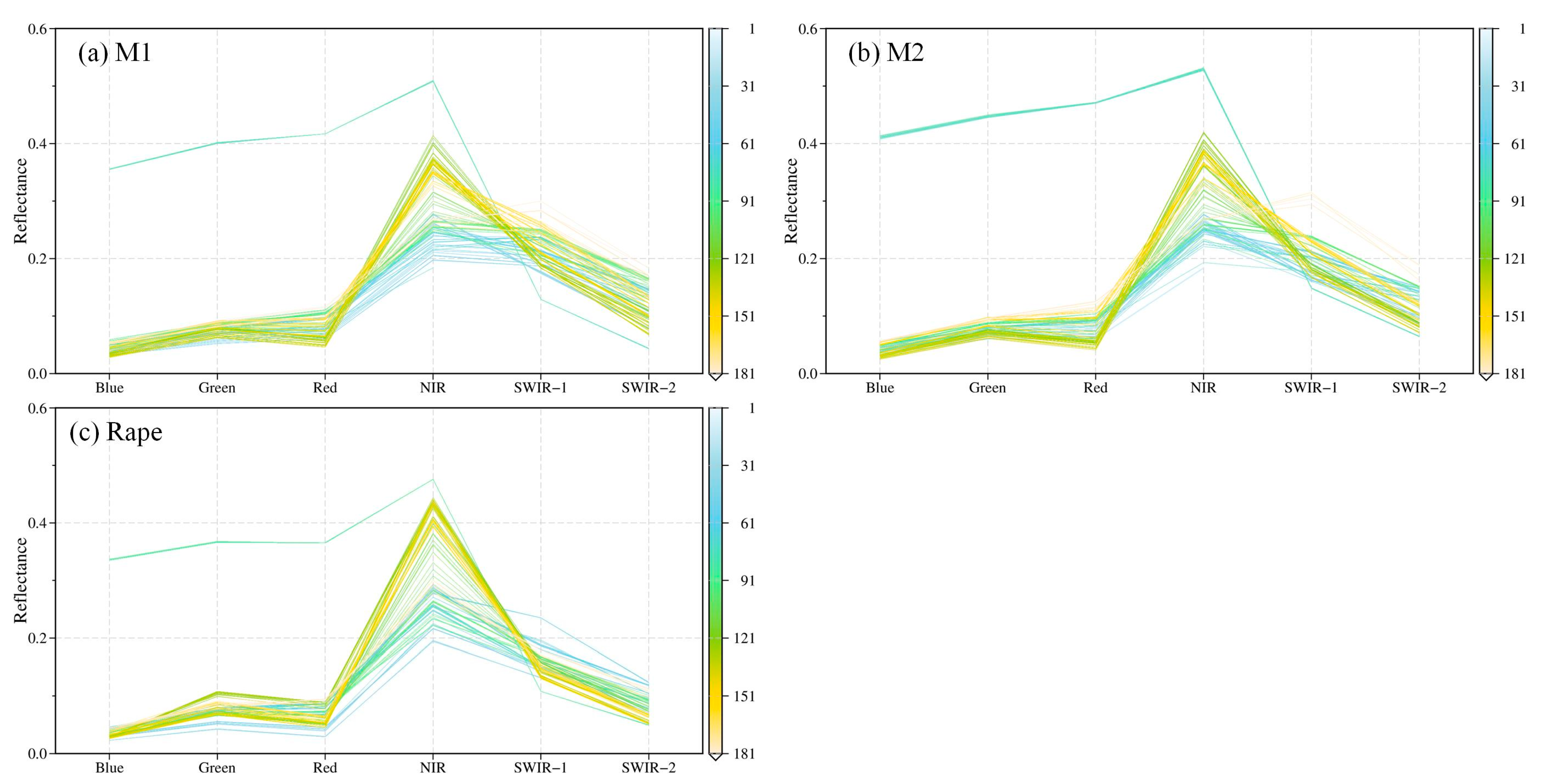
The identification performance of rape derived from this paper is compared qualitatively with the EUCROPMAP (EU) and the RapeseedMap10 (BNU) product, as shown in Figure 22. The rape for the three products is consistent in most regions, but there are differences in some regions. As can be seen from Figure 22(a1–a4), the EUCROPMAP (EU) product has misclassified results in this area, misclassifying bare land as rape, whereas the results of this paper and the RapeseedMap10 (BNU) product show no misclassification. In the irregular area at the edge of the rape field, the misclassification from the BNU and EU products occurred at the edge of the field (Figure 22(b1–b5)), while this paper identifies better. It can be seen from Figure 22(c1–c4) that the EU product identifies the region as rape. From the available Sentinel-2 images, it is hard to determine whether the region is rape. Nevertheless, through MCD43A4 data, the time-series spectral characteristics of MODIS pixel (M1 and M2) in this area are investigated to represent that this area does not reflect the spectral characteristics of rape (Figure A6). In addition, there is an omission of the BNU product, as shown in Figure 22(d1–d4), the rape area can be determined from the true color composite of Sentinel-2, and both the results derived from this paper and the EU product identified them as rape.
To further evaluate the performance of rape identification, this paper carries out a quantitative evaluation based on high-resolution images and existing rape products. Firstly, verification points are randomly arranged in the study area, and the rape in 2018 are verified with high-resolution image data through quantitative indicators such as confusion matrix and F score, with an overall accuracy of 97.5%, a Kappa coefficient of 0.94 (Table 2), and an F-score of 0.96. In addition, compared with the rape products available in 2018, the percentage of all three rape can reach 81.54%, the rape of this paper overlap by up to 89.9% with those of the BNU product, and 86.04% with those of the EU product.
5. Conclusions
Accurate and timely flowering information is needed to help understand and predict the responses of ecosystem to climate change. Based on multispectral data, the time-series spectral characteristics of different vegetation types were firstly compared. Considering both the yellowness and brightness characteristics of rape at flowering, as well as the influence of soil and snow, visible and near-infrared bands were selected for the construction of a novel yellowness index (NYI). The proposed NYI is compared with three typical different yellowness indices (the Ratio Yellowness Index, Normalized Difference Yellowness Index and Ashourloo Canola Index) at different observation scales over different yellow-flowering vegetation species using ground phenological observations. In addition, the performance of NYI is examined over Gollitz on the detection of rape field. The results show that NYI is not only highly sensitive to yellow petals during the vegetation canopy, but also easily captures the flowering period at different observation scales of Sentinel-2 and Landsat 8 and different yellow-flowering vegetation species, and accentuates flower density, as well as reduces potential noise from bright features and dark green vegetation. Taking Sentinel-2 as a reference, the yellowness index constructed performs the best among different yellowness indices at different flower densities, with a relative difference of 74% between flower densities of 33% and 78%, while that of other indices no more than 57%. In addition, the flowering status of rape can be captured more accurately and be consistent with PhenoCam observation and Deutscher Wetterdienst phenological station compared with the existing three different yellowness indices. The case study applying NYI to identify rape fields exhibits good accuracy, with the overall accuracy of 97.5%, the kappa coefficient of 0.94 and F score of 0.96. The yellowness index constructed contributes to facilitating the quantification of floral dynamics with available remote sensing observations, and is a potential index for mapping yellow-flowering vegetation and tracking long-term changes in the future. However, it also has certain shortcomings, being less sensitive to distinguishing yellow flowers from blue roofs, as well as poor effect in identifying the flowering stage of sunflower, which needs to be improved in future work.
Author Contributions
Conceptualization, Y.S. and C.S.; methodology, C.S. and Y.S.; data organization, C.S. and H.W.; writing—original draft preparation, C.S. and Y.S.; writing—review and editing, X.D., X.Z. and A.X.; supervision, Y.S.; funding acquisition, Y.S. All authors have read and agreed to the published version of the manuscript.
Funding
This research was supported by the National Key Research and Development Program of China (No. 2020YFA0608501), the National Natural Science Foundation of China (No. 42071351), the Project supported discipline innovation team of Liaoning Technical University (No. LNTU20TD-23).
Data Availability Statement
Landsat 8, Sentinel-2, MCD43A4 and EUCROPMAP 2018 are available at the Google Earth Engine (GEE) cloud platform. RapeseedMap10 is provided by Beijing Normal University and available at http://www.nesdc.org.cn/sdo/detail?id=627f82057e28172589c2e30e, accessed on 1 July 2022. The DWD phenological observation network and PhenoCam network is available at http://www.dwd.de/phaenologie, accessed on 20 May 2022 and https://phenocam.sr.unh.edu/webcam/, accessed on 20 May 2022.
Conflicts of Interest
The authors declare no conflict of interest.
Appendix A
Figure A1.
Comparison of four yellowness indices of spring rape in Zhaosu during June–August 2018, as shown by the time series of (a–c) Sentinel-2 imagery at 10m resolution (RGB), and (d–f), (g–i), (j–l), (m–o) corresponding to RYI, NDYI, ACI, NYI imagery, respectively. The zoomed-in regions are red rectangular area in Figure 8.
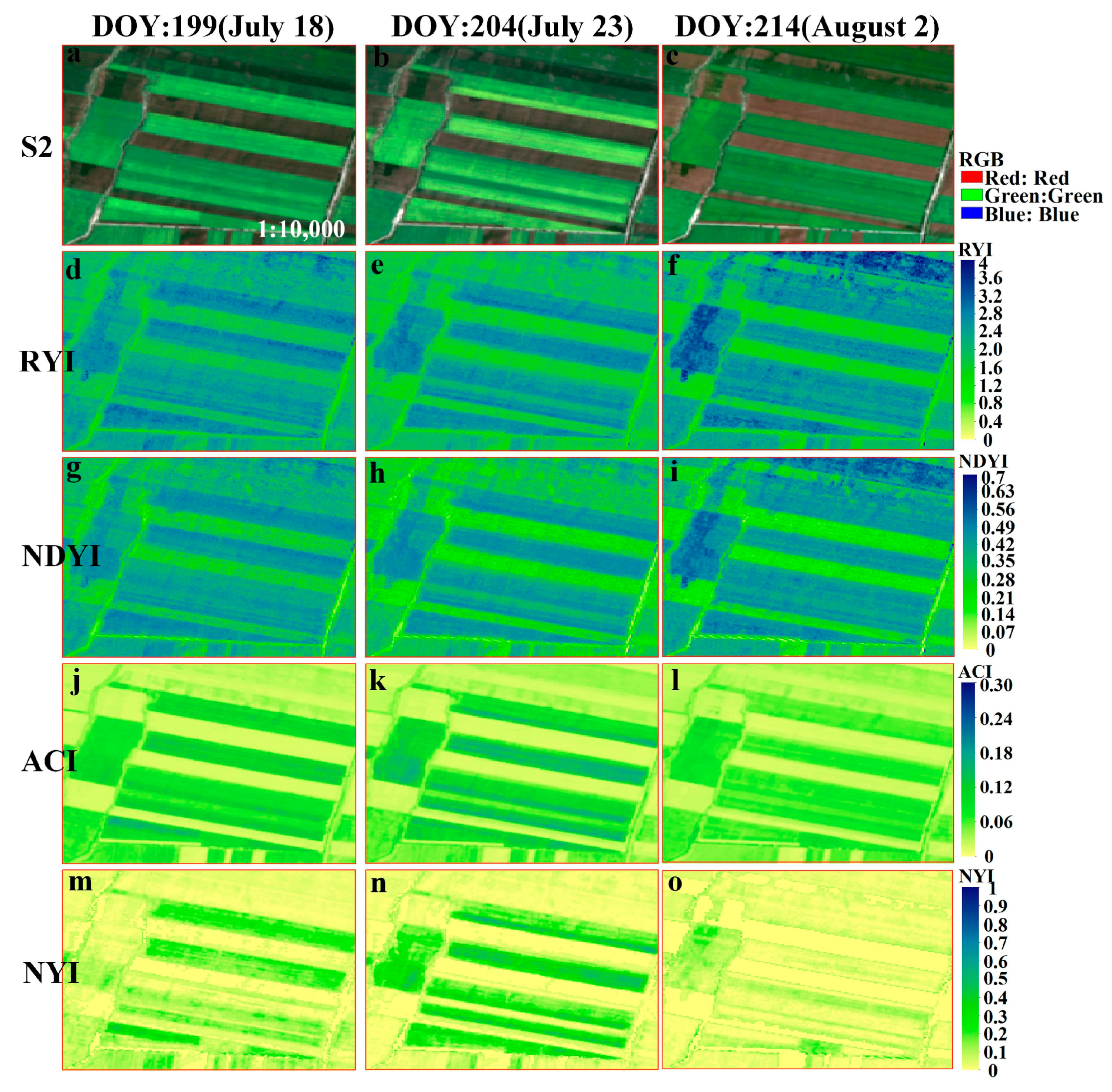
Figure A2.
Comparison of four yellowness indices of spring rape in Zhaosu during June–August 2018, as shown by the time series of (a–c) Landsat 8 imagery at 30m resolution (RGB), and (d–f), (g–i), (j–l), (m–o) corresponding to RYI, NDYI, ACI, NYI imagery, respectively. The zoomed-in regions are red rectangular area in Figure 9.
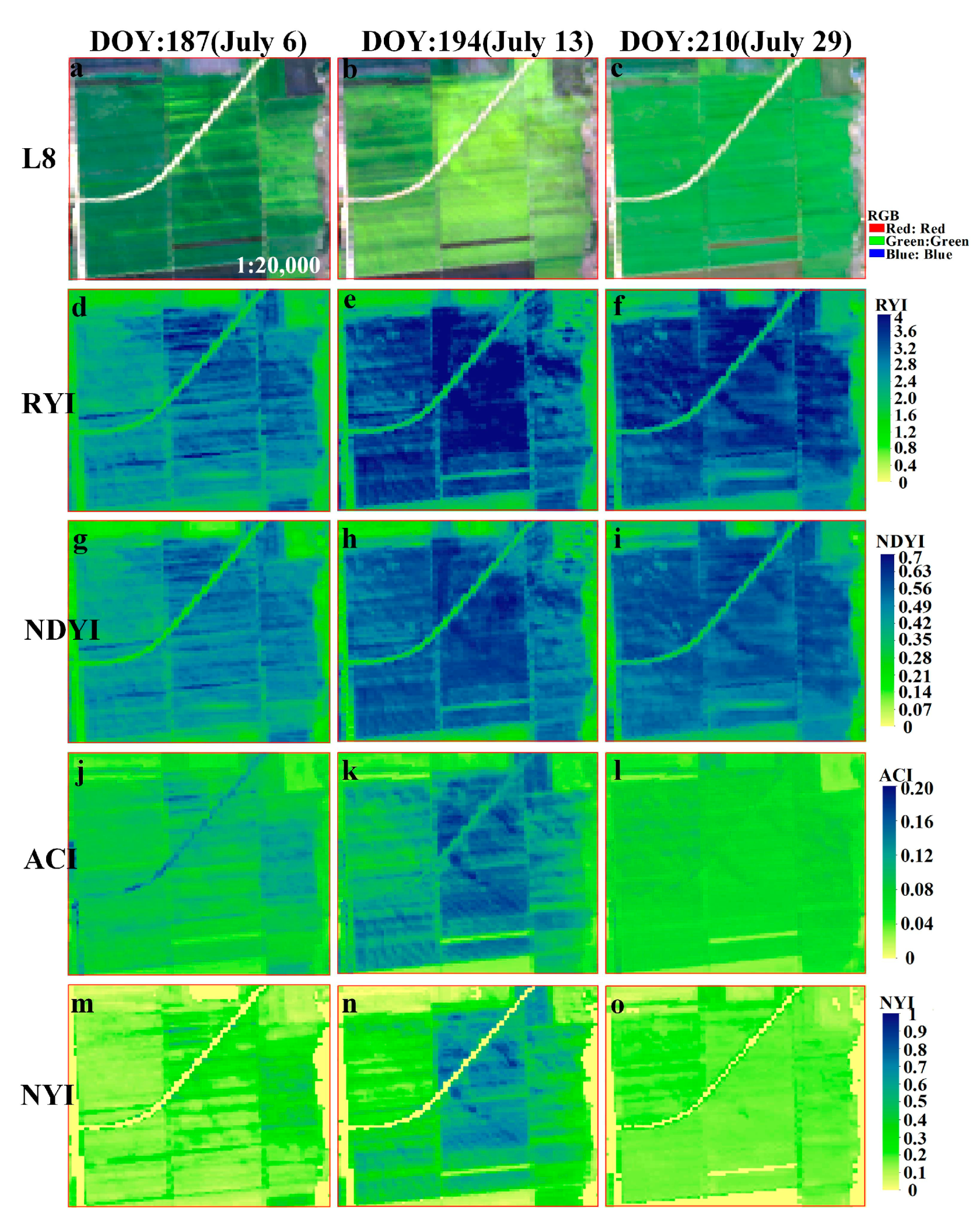
Figure A3.
Comparison of four yellowness indices of winter rape in Yanchen during January–April 2020, as shown by the time series of (a–c) Sentinel-2 (RGB), and (d–f), (g–i), (j–l), (m–o) corresponding to RYI, NDYI, ACI, NYI imagery, respectively. The zoomed-in regions are red rectangular area in Figure 10.

Figure A4.
Comparison of four yellowness indices of royal chrysanthemum in Wuyuan during October–December 2020, as shown by the time series of (a–c) Sentinel-2 (RGB), and (d–f), (g–i), (j–l), (m–o) corresponding to RYI, NDYI, ACI, NYI imagery, respectively. The zoomed-in regions are red rectangular area in Figure 15.

Figure A5.
Comparison of four yellowness indices of winter rape in Sachsen during April–May 2018, as shown by the time series of (a–c) Sentinel-2 (RGB), and (d–f), (g–i), (j–l), (m–o) corresponding to RYI, NDYI, ACI, NYI imagery, respectively. The zoomed-in regions are red rectangular area in Figure 19.
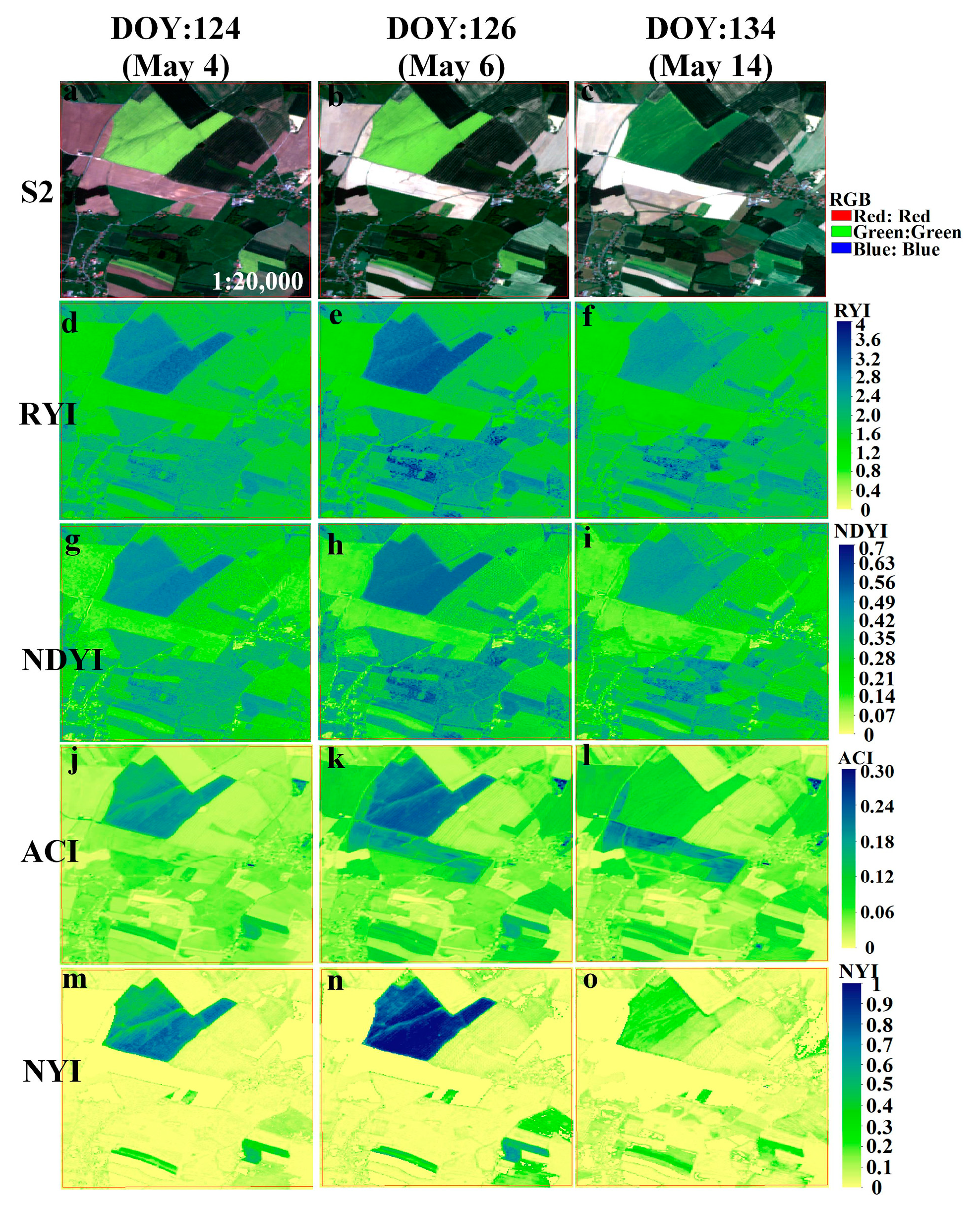
Figure A6.
Time-series spectral characteristics for ground objects of MCD43A4 at Görlitz in 2018. M1 and M2 indicate the MODIS reflectance of the cyan parallelogram area in Figure 22.
Figure A6.
Time-series spectral characteristics for ground objects of MCD43A4 at Görlitz in 2018. M1 and M2 indicate the MODIS reflectance of the cyan parallelogram area in Figure 22.
References
- Cleland, E.E.; Chuine, I.; Menzel, A.; Mooney, H.A.; Schwartz, M.D. Shifting plant phenology in response to global change. Trends Ecol. Evol. 2007, 22, 357–365. [Google Scholar] [CrossRef] [PubMed]
- Reyes-Fox, M.; Steltzer, H.; Trlica, M.J.; McMaster, G.S.; Andales, A.A.; LeCain, D.R.; Morgan, J.A. Elevated CO2 further lengthens growing season under warming conditions. Nature 2014, 510, 259–262. [Google Scholar] [CrossRef] [Green Version]
- Zhang, G.; Zhang, Y.; Dong, J.; Xiao, X. Green-up dates in the Tibetan Plateau have continuously advanced from 1982 to 2011. Proc. Natl. Acad. Sci. USA 2013, 110, 4309–4314. [Google Scholar] [CrossRef] [PubMed] [Green Version]
- Zhang, X.; Zhang, Q. Monitoring interannual variation in global crop yield using long-term AVHRR and MODIS observations. ISPRS J. Photogramm. Remote Sens. 2016, 114, 191–205. [Google Scholar] [CrossRef] [PubMed]
- Rafferty, N.E.; Ives, A.R. Effects of experimental shifts in flowering phenology on plant-pollinator interactions. Ecol. Lett. 2011, 14, 69–74. [Google Scholar] [CrossRef]
- Gezon, Z.J.; Inouye, D.W.; Irwin, R.E. Phenological change in a spring ephemeral: Implications for pollination and plant reproduction. Glob. Chang. Biol. 2016, 22, 1779–1793. [Google Scholar] [CrossRef]
- Forrest, J.R.K. Plant-pollinator interactions and phenological change: What can we learn about climate impacts from experiments and observations? Oikos 2015, 124, 4–13. [Google Scholar] [CrossRef]
- Burkle, L.A.; Marlin, J.C.; Knight, T.M. Plant-pollinator interactions over 120 years: Loss of species, co-occurrence, and function. Science 2013, 339, 1611–1615. [Google Scholar] [CrossRef] [Green Version]
- Garibaldi, L.A.; Carvalheiro, L.G.; Leonhardt, S.D.; Aizen, M.A.; Blaauw, B.R.; Isaacs, R.; Kuhlmann, M.; Kleijn, D.; Klein, A.M.; Kremen, C.; et al. From research to action: Enhancing crop yield through wild pollinators. Front. Ecol. Environ. 2014, 12, 439–447. [Google Scholar] [CrossRef] [Green Version]
- Schiessl, S.; Iniguez-Luy, F.; Qian, W.; Snowdon, R.J. Diverse regulatory factors associate with flowering time and yield responses in winter-type Brassica napus. BMC Genom. 2015, 16, 737. [Google Scholar] [CrossRef] [Green Version]
- Stratonovitch, P.; Semenov, M.A. Heat tolerance around flowering in wheat identified as a key trait for increased yield potential in Europe under climate change. J. Exp. Bot. 2015, 66, 3599–3609. [Google Scholar] [CrossRef] [PubMed] [Green Version]
- Craufurd, P.Q.; Wheeler, T.R. Climate change and the flowering time of annual crops. J. Exp. Bot. 2009, 60, 2529–2539. [Google Scholar] [CrossRef] [PubMed] [Green Version]
- Dixon, D.J.; Callow, J.N.; Duncan, J.M.A.; Setterfield, S.A.; Pauli, N. Satellite prediction of forest flowering phenology. Remote Sens. Environ. 2021, 255, 112197. [Google Scholar] [CrossRef]
- Shuai, Y.; Schaaf, C.; Zhang, X.; Strahler, A.; Roy, D.; Morisette, J.; Wang, Z.; Nightingale, J.; Nickeson, J.; Richardson, A.D.; et al. Daily MODIS 500 m reflectance anisotropy direct broadcast (DB) products for monitoring vegetation phenology dynamics. Int. J. Remote Sens. 2013, 34, 5997–6016. [Google Scholar] [CrossRef]
- Misra, G.; Cawkwell, F.; Wingler, A. Status of Phenological Research Using Sentinel-2 Data: A Review. Remote Sens. 2020, 12, 2760. [Google Scholar] [CrossRef]
- Chen, B.; Jin, Y.F.; Brown, P. An enhanced bloom index for quantifying floral phenology using multi-scale remote sensing observations. ISPRS J. Photogramm. Remote Sens. 2019, 156, 108–120. [Google Scholar] [CrossRef]
- Sulik, J.J.; Long, D.S. Spectral indices for yellow canola flowers. Int. J. Remote Sens. 2015, 36, 2751–2765. [Google Scholar] [CrossRef]
- Sulik, J.J.; Long, D.S. Spectral considerations for modeling yield of canola. Remote Sens. Environ. 2016, 184, 161–174. [Google Scholar] [CrossRef] [Green Version]
- D’Andrimont, R.; Taymans, M.; Lemoine, G.; Ceglar, A.; Yordanov, M.; van der Velde, M. Detecting flowering phenology in oil seed rape parcels with Sentinel-1 and -2 time series. Remote Sens. Environ. 2020, 239, 111660. [Google Scholar] [CrossRef]
- Han, J.; Zhang, Z.; Cao, J. Developing a New Method to Identify Flowering Dynamics of Rapeseed Using Landsat 8 and Sentinel-1/2. Remote Sens. 2021, 13, 105. [Google Scholar] [CrossRef]
- Ashourloo, D.; Shahrabi, H.S.; Azadbakht, M.; Aghighi, H.; Nematollahi, H.; Alimohammadi, A.; Matkan, A.A. Automatic canola mapping using time series of sentinel 2 images. ISPRS J. Photogramm. Remote Sens. 2019, 156, 63–76. [Google Scholar] [CrossRef]
- Tian, H.; Chen, T.; Li, Q.; Mei, Q.; Wang, S.; Yang, M.; Wang, Y.; Qin, Y. A Novel Spectral Index for Automatic Canola Mapping by Using Sentinel-2 Imagery. Remote Sens. 2022, 14, 1113. [Google Scholar] [CrossRef]
- Rengarajan, R.; Choate, M.; Storey, J.; Franks, S.; Micijevic, E. Landsat Collection-2 geometric calibration updates. In Proceedings of the Earth Observing Systems XXV, Online, 24 August–4 September 2020; pp. 85–95. [Google Scholar]
- Languille, F.; Déchoz, C.; Gaudel, A.; Greslou, D.; De Lussy, F.; Trémas, T.; Poulain, V. Sentinel-2 geometric image quality commissioning: First results. In Proceedings of the Image and Signal Processing for Remote Sensing XXI, Toulouse, France, 21–23 September 2015; pp. 61–73. [Google Scholar]
- D’Andrimont, R.; Verhegghen, A.; Lemoine, G.; Kempeneers, P.; Meroni, M.; van der Velde, M. From parcel to continental scale—A first European crop type map based on Sentinel-1 and LUCAS Copernicus in-situ observations. Remote Sens. Environ. 2021, 266, 112708. [Google Scholar] [CrossRef]
- Han, J.; Zhang, Z.; Luo, Y.; Cao, J.; Zhang, L.; Zhang, J.; Li, Z. Developing a phenology-and pixel-based algorithm for mapping rapeseed at 10m spatial resolution using multi-source data. Earth Syst. Sci. Data 2021, 2021, 1–31. [Google Scholar] [CrossRef]
- Kaspar, F.; Zimmermann, K.; Polte-Rudolf, C. An overview of the phenological observation network and the phenological database of Germany’s national meteorological service (Deutscher Wetterdienst). Adv. Sci. Res. 2015, 11, 93–99. [Google Scholar] [CrossRef] [Green Version]
- Böttcher, U.; Rampin, E.; Hartmann, K.; Zanetti, F.; Flenet, F.; Morison, M.; Kage, H. A phenological model of winter oilseed rape according to the BBCH scale. Crop Pasture Sci. 2016, 67, 345–358. [Google Scholar] [CrossRef]
- Richardson, A.D.; Hufkens, K.; Milliman, T.; Aubrecht, D.M.; Chen, M.; Gray, J.M.; Johnston, M.R.; Keenan, T.F.; Klosterman, S.T.; Kosmala, M.; et al. Tracking vegetation phenology across diverse North American biomes using PhenoCam imagery. Sci. Data 2018, 5, 180028. [Google Scholar] [CrossRef]
- Wilson, J.; Zhang, C.; Kovacs, J. Separating Crop Species in Northeastern Ontario Using Hyperspectral Data. Remote Sens. 2014, 6, 925–945. [Google Scholar] [CrossRef] [Green Version]
- Yates, D.J.; Steven, M.D. Reflexion and absorption of solar radiation by flowering canopies of oil-seed rape (Brassica napus L.). J. Agric. Sci.-Camb. 2009, 109, 495–502. [Google Scholar] [CrossRef]
- Migdall, S.; Ohl, N.; Bach, H. Parameterisation of the Land Surface Reflectance Model SLC for Winter Rape Using Spaceborne Hyperspectral CHRIS Data. In Proceedings of the Hyperspectral 2010 Workshop, Frascati, Italy, 17–19 March 2010. [Google Scholar]
- Wójtowicz, M.; Wójtowicz, A.; Piekarczyk, J. Application of remote sensing methods in agriculture. Commun. Biometry Crop Sci. 2016, 11, 31–50. [Google Scholar]
- Shen, M.; Chen, J.; Zhu, X.; Tang, Y. Yellow flowers can decrease NDVI and EVI values: Evidence from a field experiment in an alpine meadow. Can. J. Remote Sens. 2014, 35, 99–106. [Google Scholar] [CrossRef]
- Wang, D.; Fang, S.; Yang, Z.; Wang, L.; Tang, W.; Li, Y.; Tong, C. A Regional Mapping Method for Oilseed Rape Based on HSV Transformation and Spectral Features. ISPRS Int. J. Geo-Inf. 2018, 7, 224. [Google Scholar] [CrossRef] [Green Version]
- Zhang, T.; Vail, S.; Duddu, H.S.N.; Parkin, I.A.P.; Guo, X.; Johnson, E.N.; Shirtliffe, S.J. Phenotyping Flowering in Canola (Brassica napus L.) and Estimating Seed Yield Using an Unmanned Aerial Vehicle-Based Imagery. Front. Plant Sci. 2021, 12, 686332. [Google Scholar] [CrossRef] [PubMed]
Figure 1.
Locations of the study area in Zhaosu (a), Hanzhong (b), Yancheng (c), Jingmen (d), Wuyuan (e) of China (A), USA (B), and Germany (C).
Figure 1.
Locations of the study area in Zhaosu (a), Hanzhong (b), Yancheng (c), Jingmen (d), Wuyuan (e) of China (A), USA (B), and Germany (C).

Figure 2.
Technology roadmap in this study.

Figure 3.
The spectral characteristics on different DOY for typical features of Sentinel-2 at Zhaosu in 2019, of (a) rape-1, (b) rape-2, (c) wheat, (d) forest, (e) maize, (f) soybean, as well as true color composites (red, green, and blue) of time series of Sentinel-2 imagery for rape-1 (a1–a3), rape-2 (b1–b3), and wheat (c1–c3). Note: rape-1 and rape-2 bloom at DOY:190 and DOY:205.
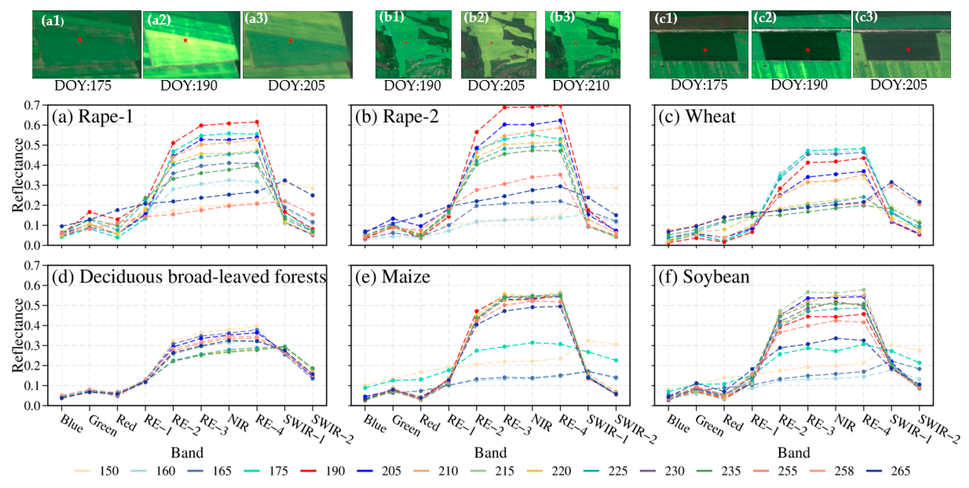
Figure 4.
The spectral characteristics on different DOY for rape from Sentinel-2 at Hanzhong and Yancheng in 2021. Note: both rape-1 and rape-2 of Hanzhong blooms at DOY:83. Both rape-1 and rape-2 of Yancheng bloom at DOY:87.
Figure 4.
The spectral characteristics on different DOY for rape from Sentinel-2 at Hanzhong and Yancheng in 2021. Note: both rape-1 and rape-2 of Hanzhong blooms at DOY:83. Both rape-1 and rape-2 of Yancheng bloom at DOY:87.

Figure 5.
Image for the yellowness index function of (a) , (b) .
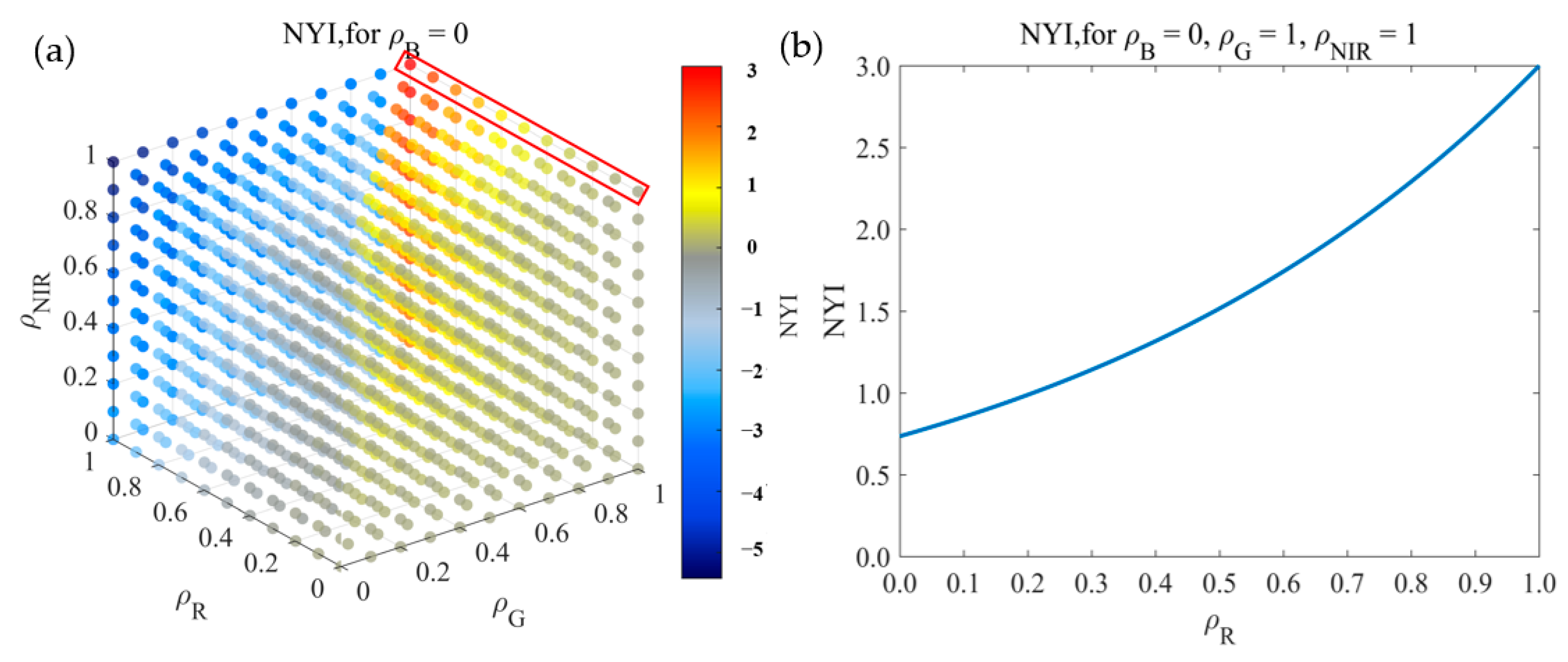
Figure 6.
Time-series characteristics of the NYI for typical features based on Sentinel-2 in (a) Zhaosu, (b) Hanzhong, (c) Yancheng, and (d) Wuyuan.
Figure 6.
Time-series characteristics of the NYI for typical features based on Sentinel-2 in (a) Zhaosu, (b) Hanzhong, (c) Yancheng, and (d) Wuyuan.
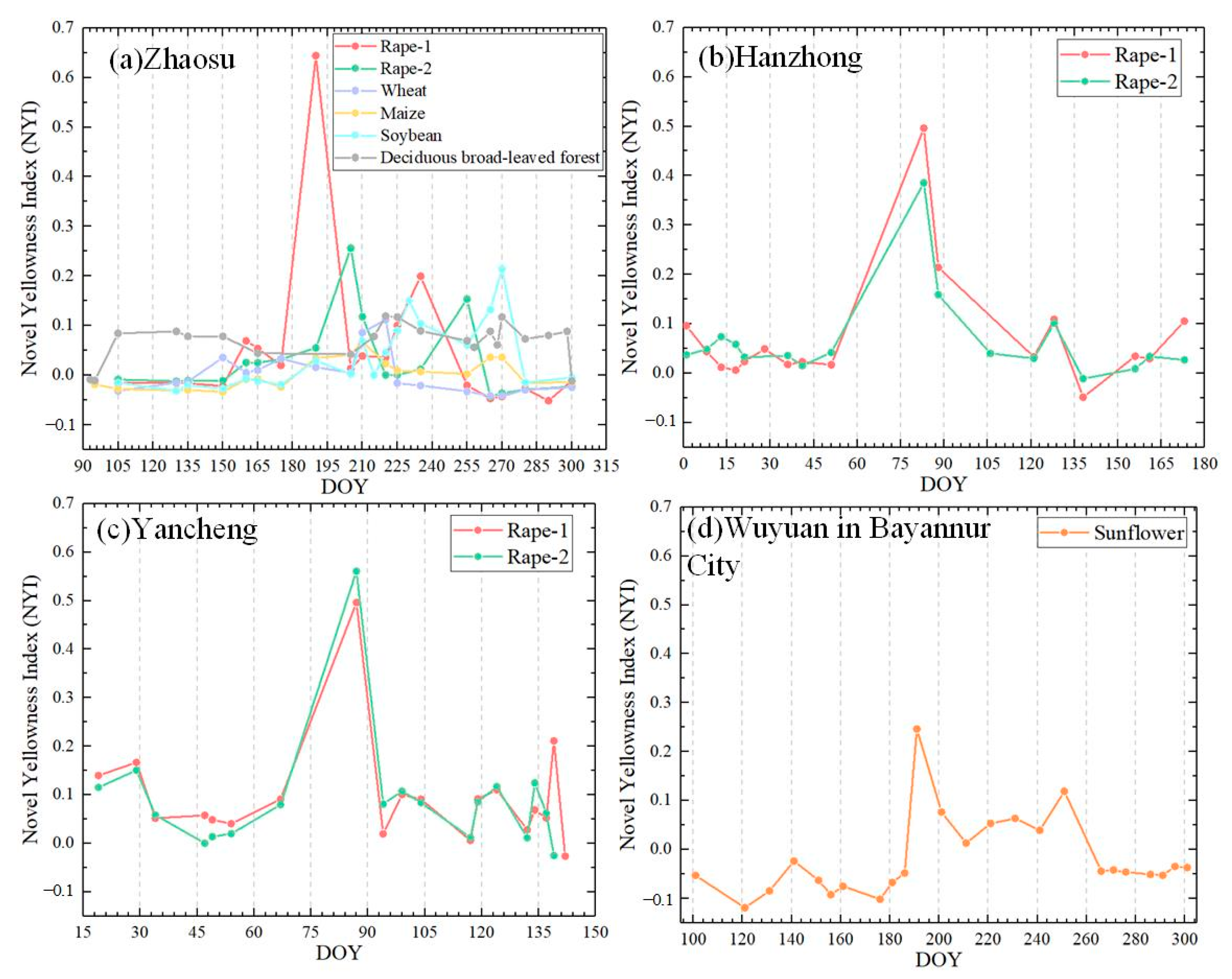
Figure 7.
Time-series characteristics of the NYI for typical features in Northeast China based on MCD43A4 of (a) soybean, (b) wheat, (c) maize, (d) paddy, (e) forest (mixed coniferous-deciduous broad-leaved forest), and (f) grassland.
Figure 7.
Time-series characteristics of the NYI for typical features in Northeast China based on MCD43A4 of (a) soybean, (b) wheat, (c) maize, (d) paddy, (e) forest (mixed coniferous-deciduous broad-leaved forest), and (f) grassland.
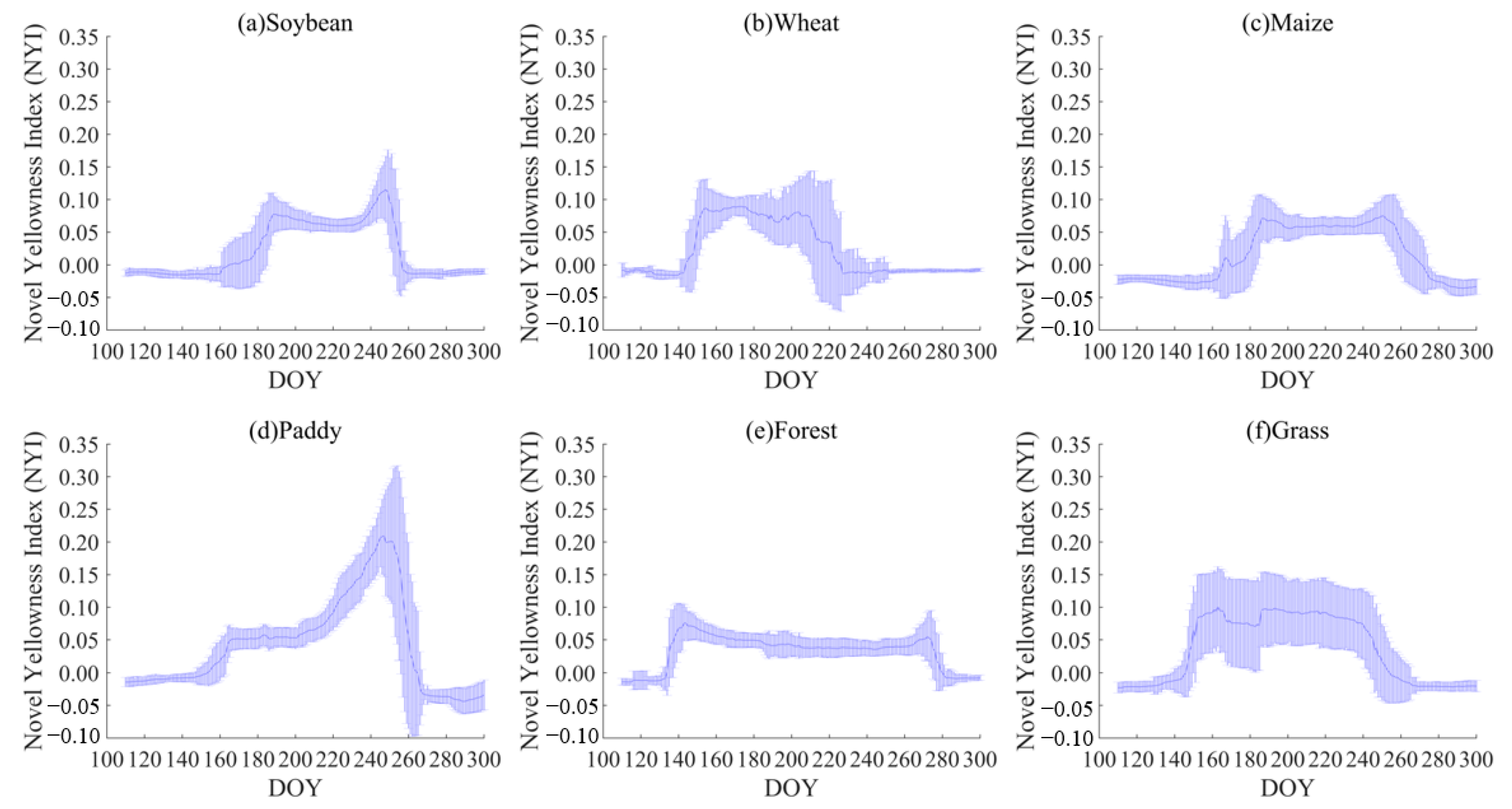
Figure 8.
Comparison of four yellowness indices of spring rape in Zhaosu during June–August 2021, as shown by the time series of (a–e) Sentinel-2 imagery at 10m resolution (RGB), and (f–j), (k–o), (p–t), (u–y) corresponding to RYI, NDYI, ACI, NYI imagery, respectively. Note: the red rectangular area (c–e) is shown enlarged in Figure A1 of Appendix A.
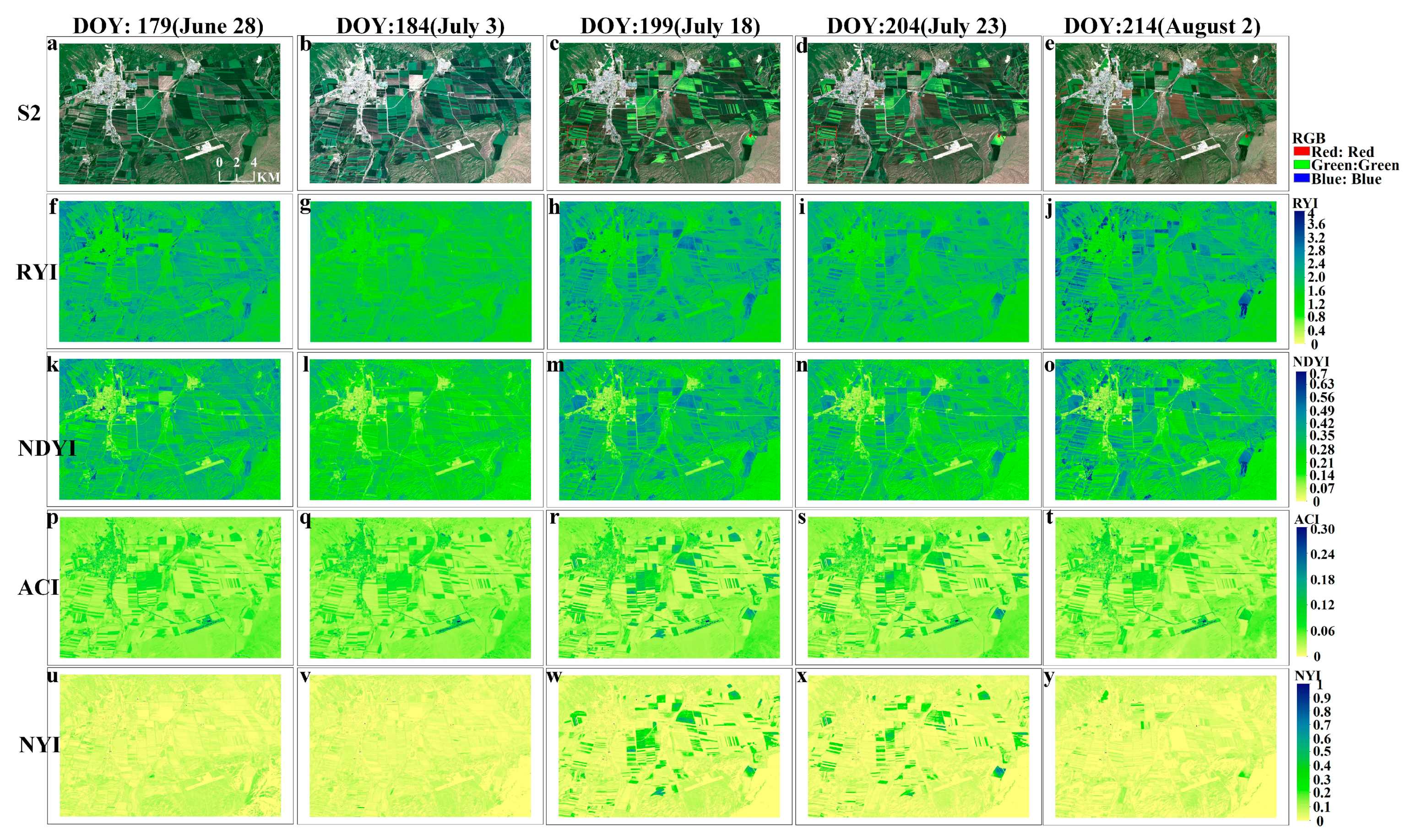
Figure 9.
Comparison of four yellowness indices of spring rape in Zhaosu during June–August 2021, as shown by the time series of (a–e) Landsat 8 imagery at 30 m resolution (RGB), and (f–j), (k–o), (p–t), (u–y) corresponding to RYI, NDYI, ACI, NYI imagery, respectively. Note: the red rectangular area (b–d) is shown enlarged in Figure A2 of Appendix A.
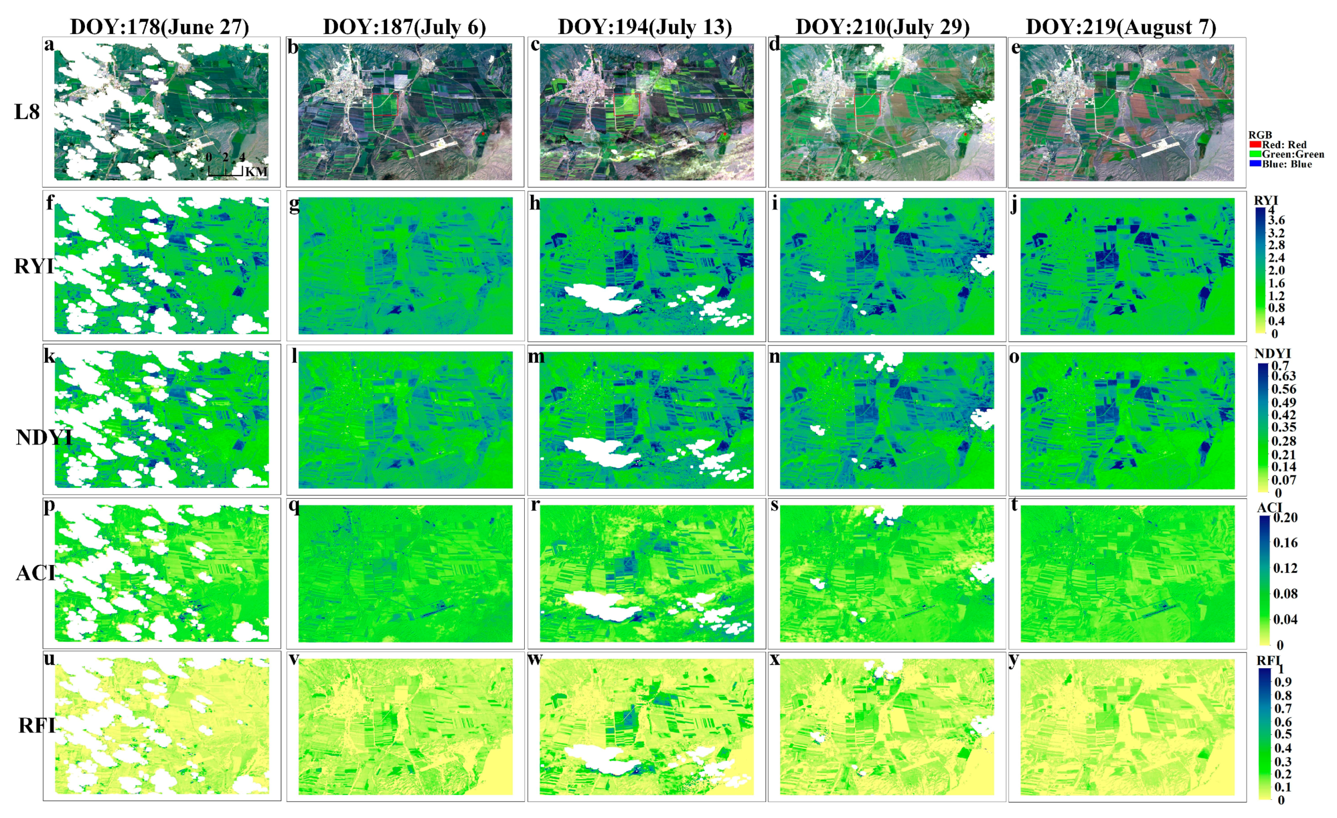
Figure 10.
Time-series characteristics of four yellowness indices for spring rape in Zhaosu in 2021 at Landsat 8 (a) and Sentinel-2 (b).
Figure 10.
Time-series characteristics of four yellowness indices for spring rape in Zhaosu in 2021 at Landsat 8 (a) and Sentinel-2 (b).
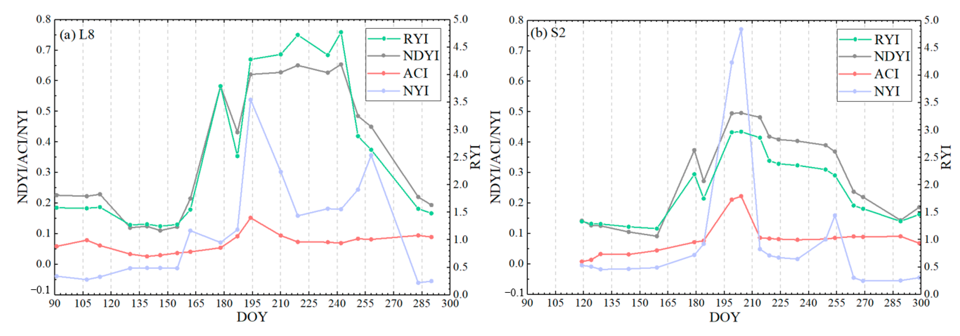
Figure 11.
Comparison of four yellowness indices of winter rape in Yanchen during January–April 2020, as shown by the time series of (a–e) Sentinel-2 (RGB), and (f–j), (k–o), (p–t), (u–y) corresponding to RYI, NDYI, ACI, NYI imagery, respectively. Note: the red rectangular area (b–d) is shown enlarged in Figure A3 of Appendix A.

Figure 12.
Comparison of four yellowness indices of winter rape in Jingmen during February–April 2020, as shown by the time series of (a–c) Sentinel-2 (RGB), and (d–f), (g–i), (j–l), (m–o) corresponding to RYI, NDYI, ACI, NYI imagery, respectively.
Figure 12.
Comparison of four yellowness indices of winter rape in Jingmen during February–April 2020, as shown by the time series of (a–c) Sentinel-2 (RGB), and (d–f), (g–i), (j–l), (m–o) corresponding to RYI, NDYI, ACI, NYI imagery, respectively.
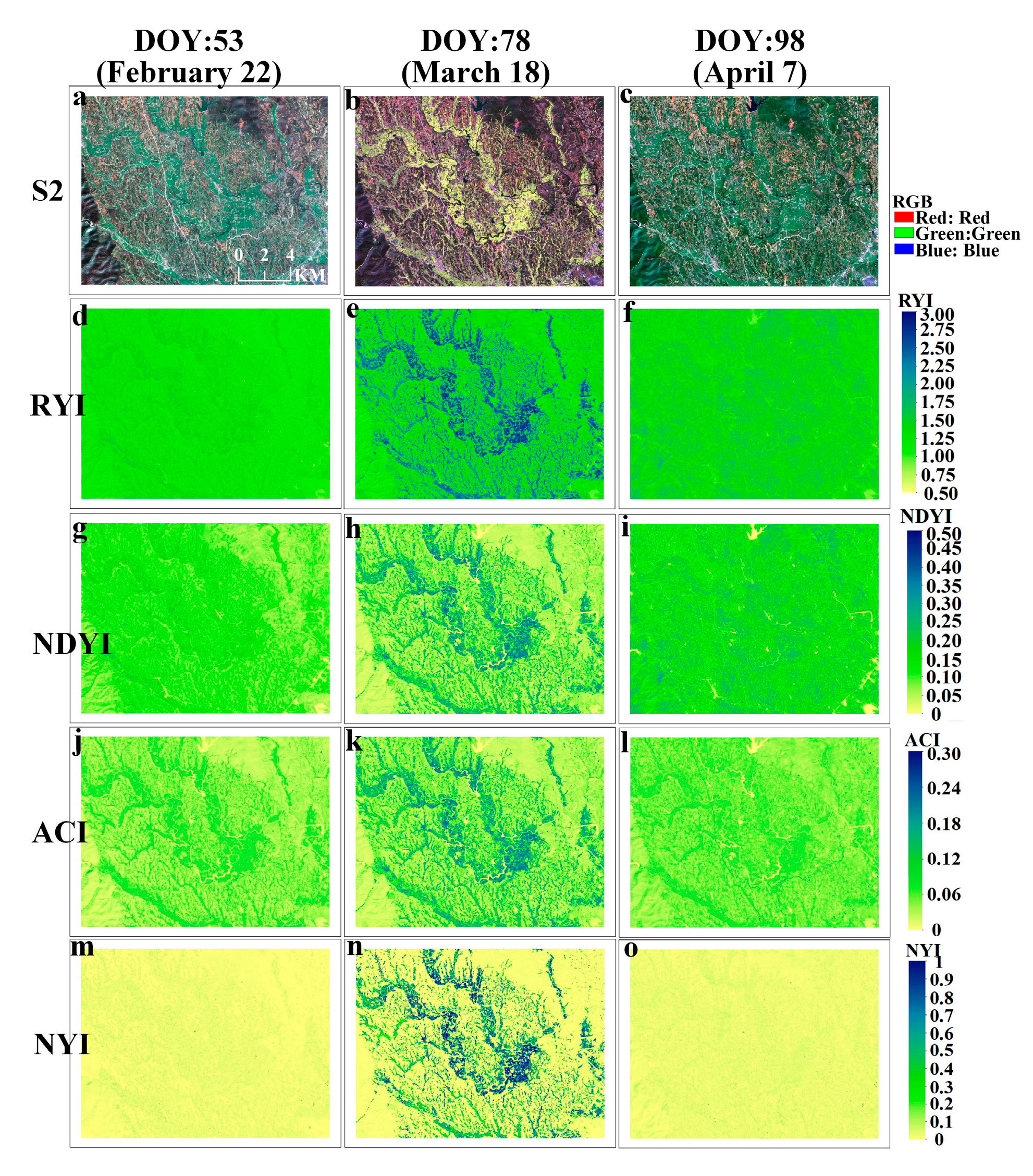
Figure 13.
Comparison of four yellowness indices of royal chrysanthemum in Wuyuan during October–December 2020, as shown by the time series of (a–e) Sentinel-2 (RGB), and (f–j), (k–o), (p–t), (u–y) corresponding to RYI, NDYI, ACI, NYI imagery, respectively. Note: the red rectangular area (b–d) is shown enlarged in Figure A4 of Appendix A.

Figure 14.
Time-series characteristics of four yellowness indices for winter rape based on Sentinel-2 in Yancheng.
Figure 14.
Time-series characteristics of four yellowness indices for winter rape based on Sentinel-2 in Yancheng.
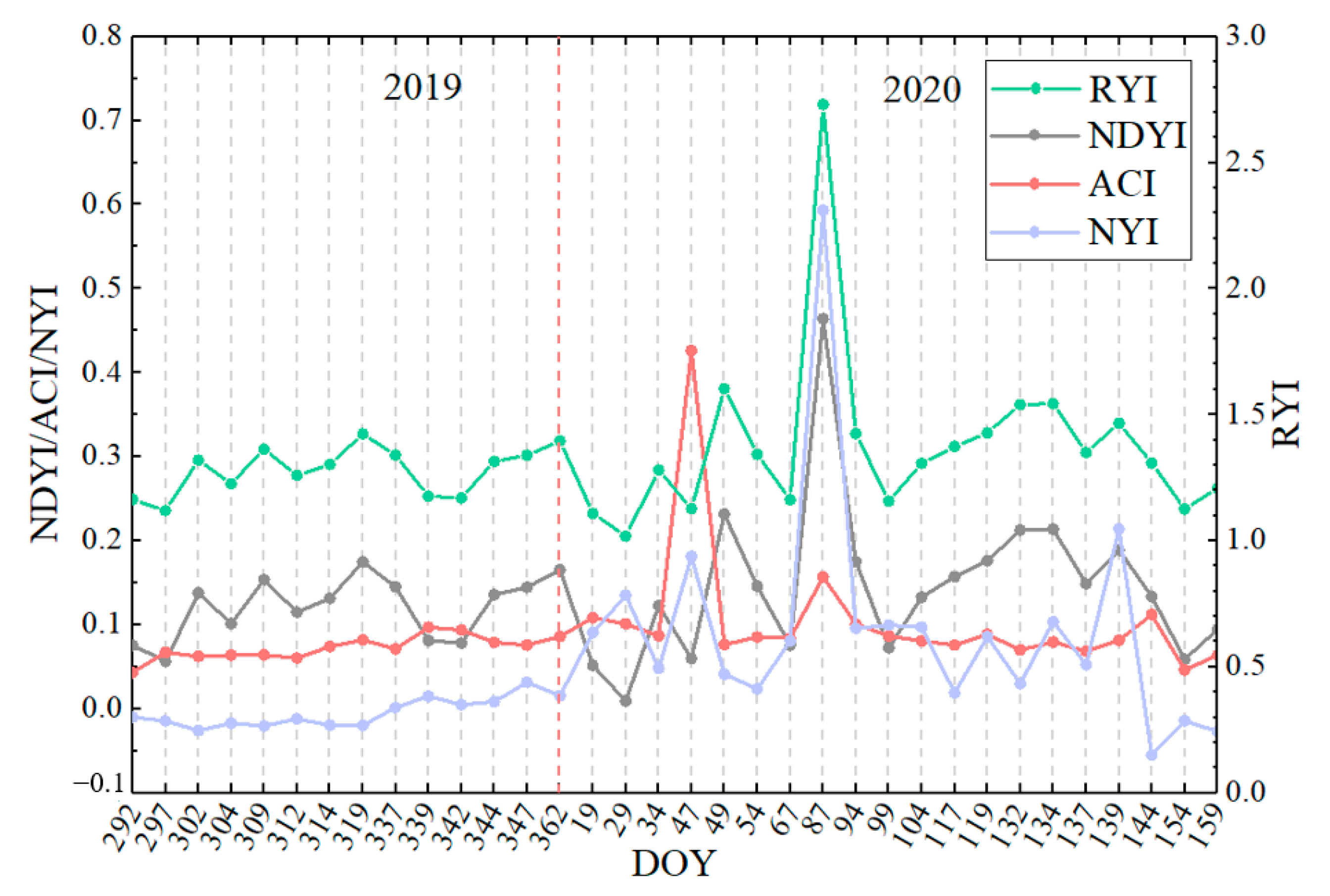
Figure 15.
Time-series characteristics of four yellowness indices for winter rape based on Sentinel-2 in Jingmen.
Figure 15.
Time-series characteristics of four yellowness indices for winter rape based on Sentinel-2 in Jingmen.
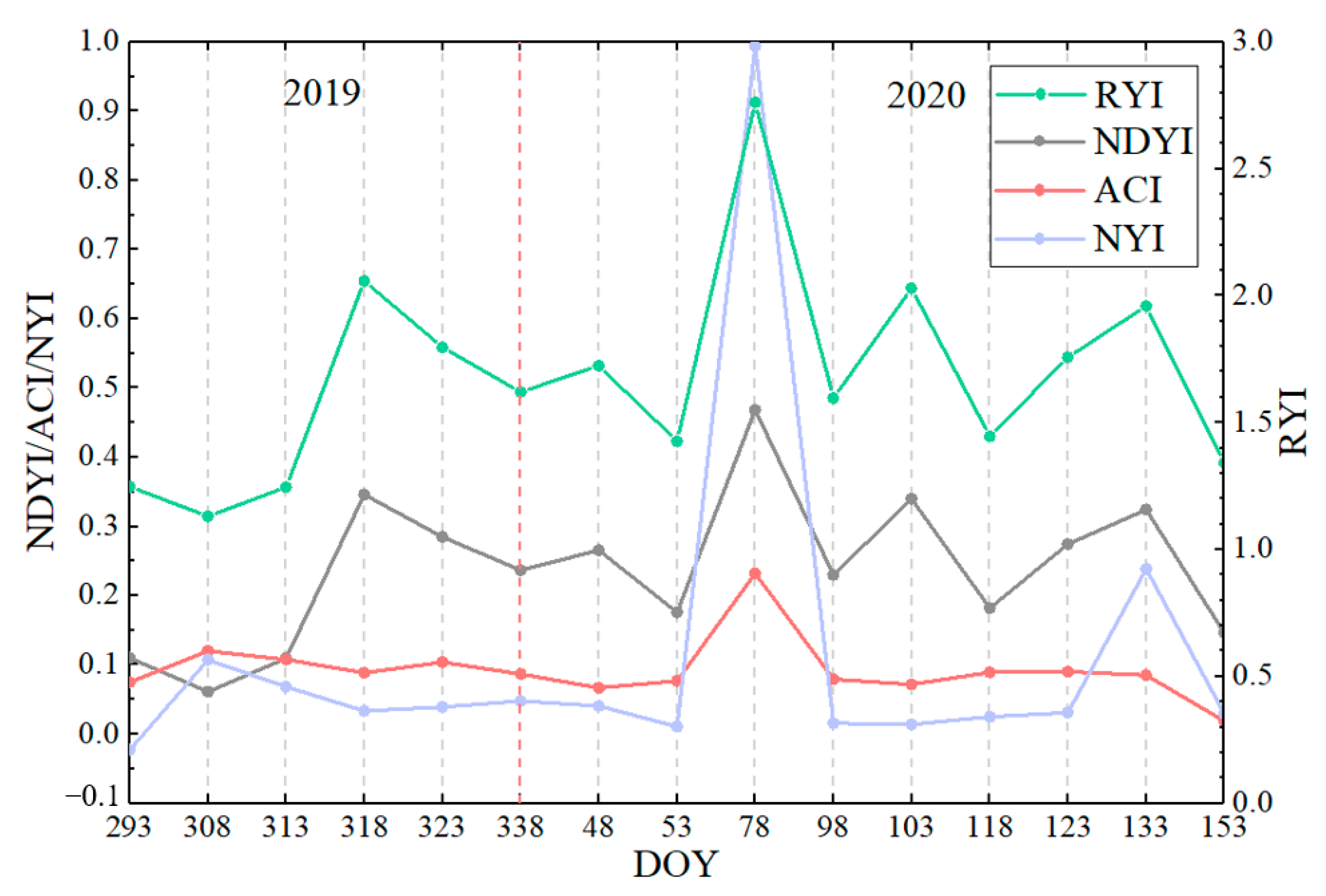
Figure 16.
Time-series characteristics of four yellowness indices for royal chrysanthemum based on Sentinel-2 in Wuyuan.
Figure 16.
Time-series characteristics of four yellowness indices for royal chrysanthemum based on Sentinel-2 in Wuyuan.

Figure 17.
Different flowering coverage of rape in Landsat 8 (b,d,f) corresponding to Sentinel-2 (a,c,e) as a reference image, with (a,b) coverage 100%, (c,d) coverage 77.78%, and (e,f) coverage 33.33%. Note that the cyan areas are examples of selected samples.
Figure 17.
Different flowering coverage of rape in Landsat 8 (b,d,f) corresponding to Sentinel-2 (a,c,e) as a reference image, with (a,b) coverage 100%, (c,d) coverage 77.78%, and (e,f) coverage 33.33%. Note that the cyan areas are examples of selected samples.

Figure 18.
Relative differences in different yellowness indices for changes in different flower densities, where Diversity_33_77 indicates the relative difference in yellowness indices as coverage changes from 33.33% to 77.78%, and Diversity_77_100 indicates the relative difference in yellowness indices as coverage changes from 77.78% to 100%.
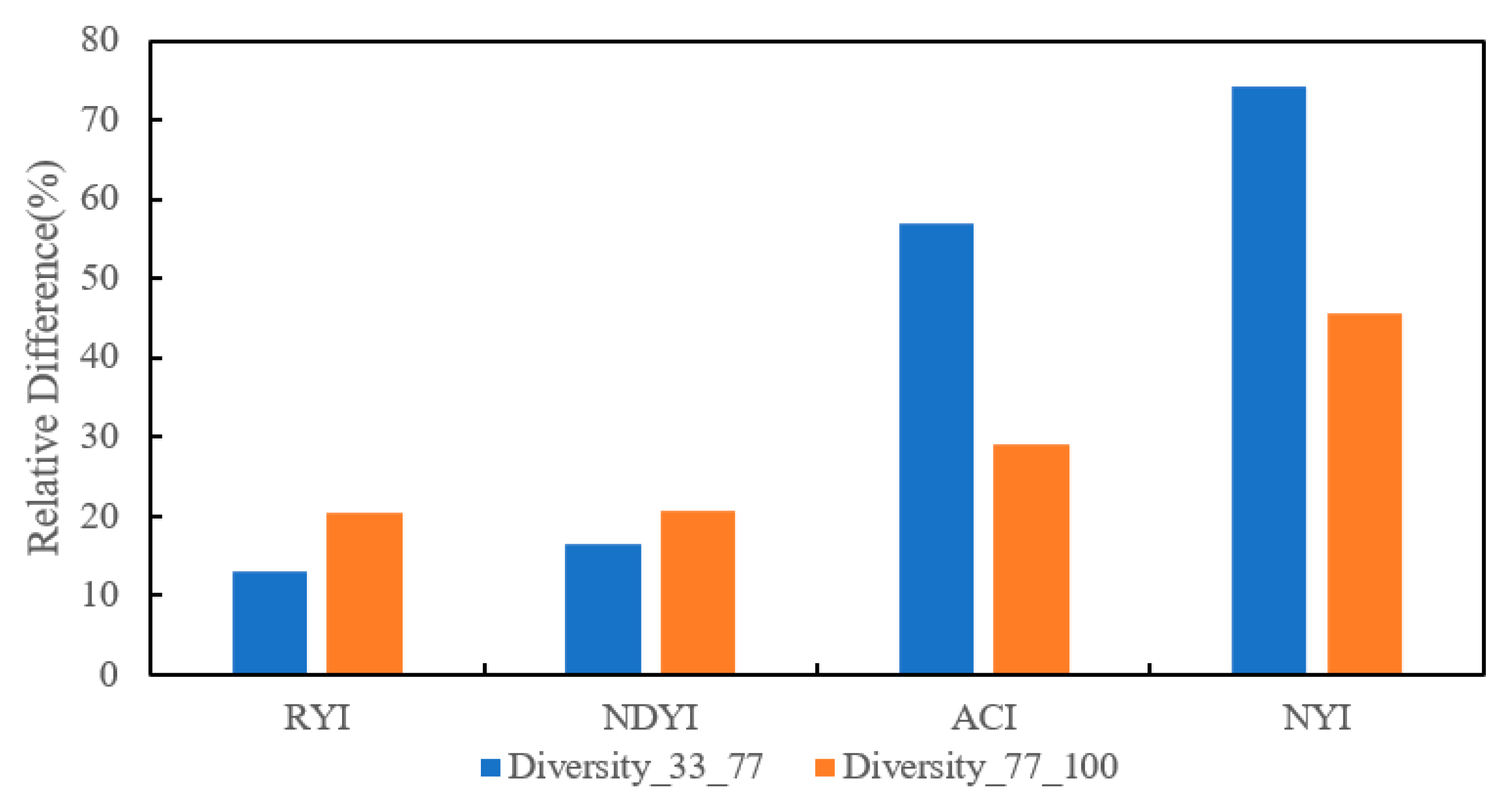
Figure 19.
Comparison of four yellowness indices of winter rape in Sachsen during April–May 2018, as shown by the time series of (a–e) Sentinel-2 (RGB) and (f–j), (k–o), (p–t), (u–y) corresponding to RYI, NDYI, ACI, NYI imagery, respectively. Note: the red ellipse is the 5 km buffer zone. The red rectangular area (b–d) is shown enlarged in Figure A5 of Appendix A.
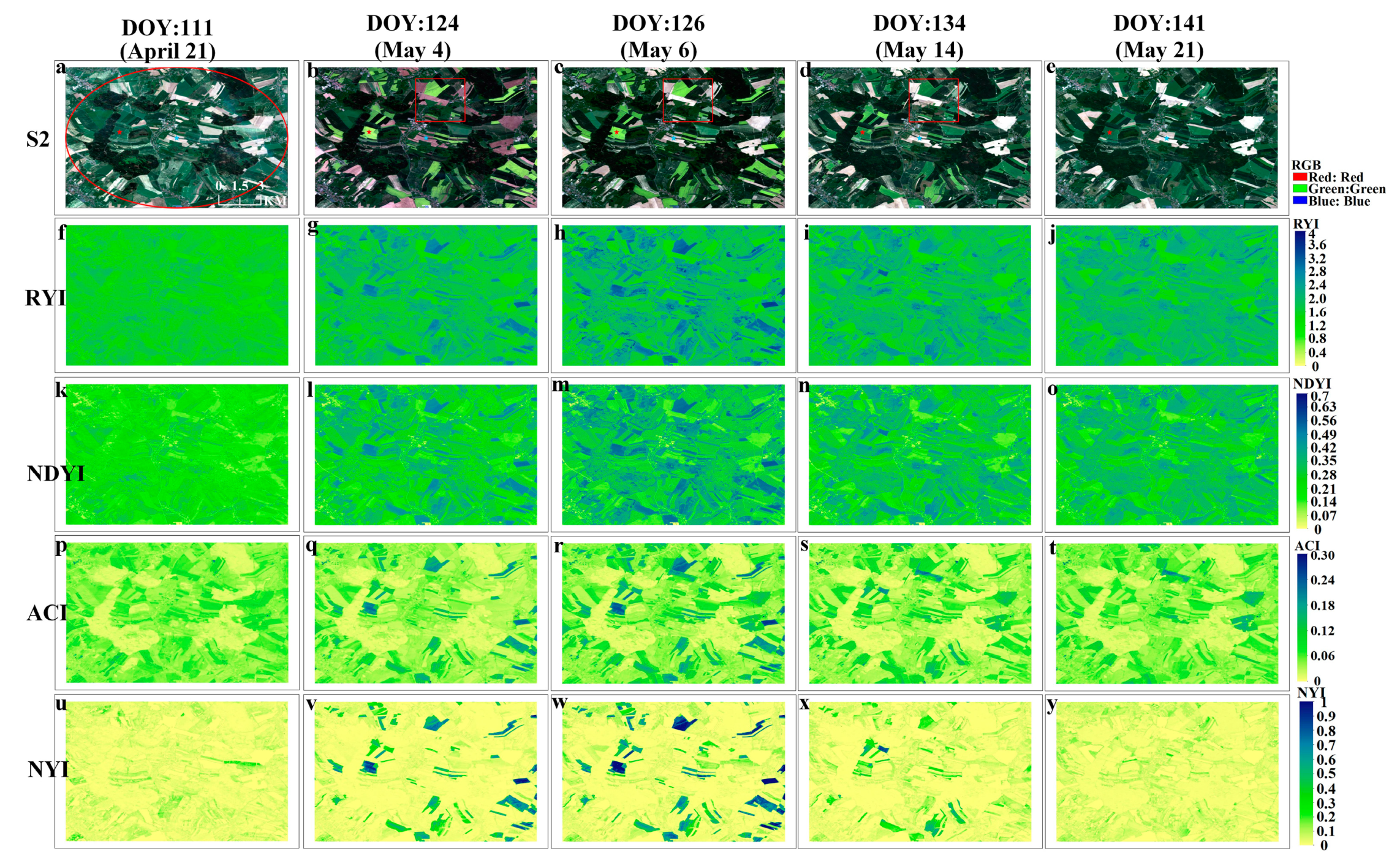
Figure 20.
Time-series characteristics of four yellowness indices for winter rape based on Sentinel-2 at DWD station (ID:12917) of Sachsen in 2018. Note: grey shaded area indicates rape flowering period provided by DWD station.
Figure 20.
Time-series characteristics of four yellowness indices for winter rape based on Sentinel-2 at DWD station (ID:12917) of Sachsen in 2018. Note: grey shaded area indicates rape flowering period provided by DWD station.
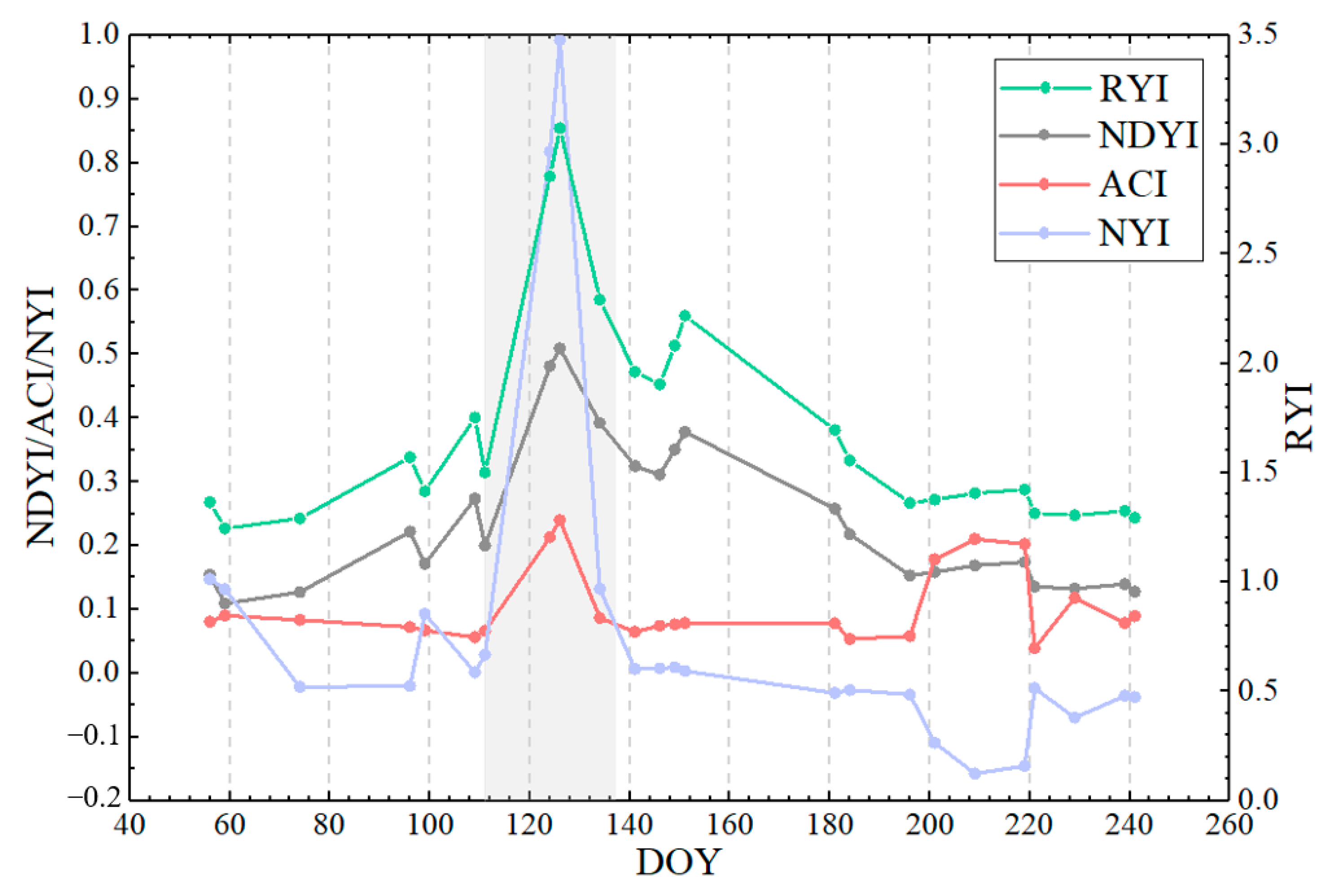
Figure 21.
Time-series characteristics of four yellowness indices for spring rape based on Sentinel-2 at cafcookeastltar01 (A), cafcookwestltar01 (B), and cafboydnorthltar01 (C) in 2021. Note: grey shaded area indicates rape flowering period provided by phenological stations.
Figure 21.
Time-series characteristics of four yellowness indices for spring rape based on Sentinel-2 at cafcookeastltar01 (A), cafcookwestltar01 (B), and cafboydnorthltar01 (C) in 2021. Note: grey shaded area indicates rape flowering period provided by phenological stations.
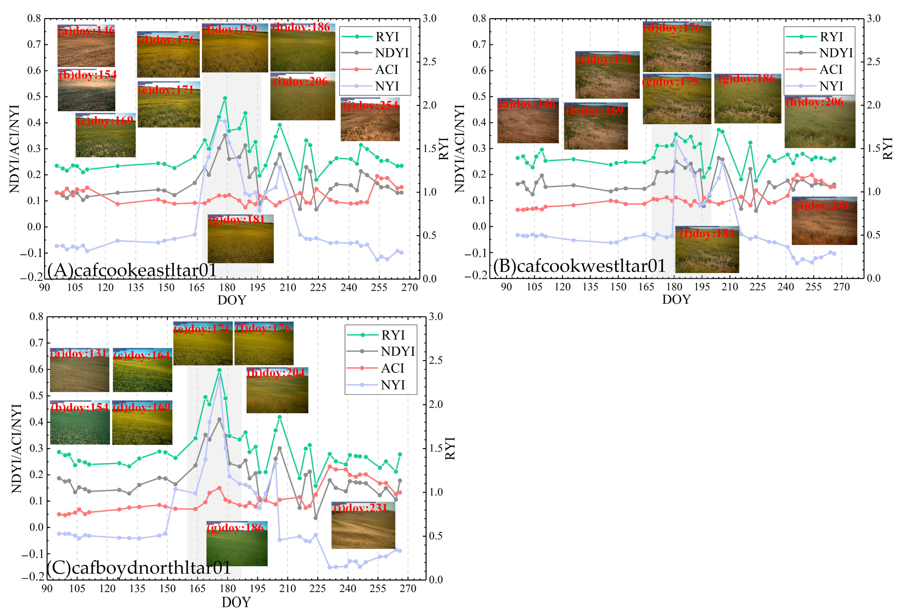
Figure 22.
Rape comparison of this paper with BNU and EU product in Görlitz, 2018. (a–d) represent the case regions labeled in (A) with four red boxes as shown by (a1,b1,b2,c1–c3,d1) Sentinel-2 imagery at 10 m resolution (RGB), and (a2,b3,c4,d2), (a3,b4,c5,d3), (a4,b5,c6,d4) corresponding to the rape of this paper, BNU, and EU, respectively. Note: R1, R2, R3 indicate that the percentage of all three products being rape, both this paper and the BNU being rape, both this paper and the EU being rape, respectively. The cyan parallelogram area (M1–M2) is shown in Figure A6 of the Appendix A.
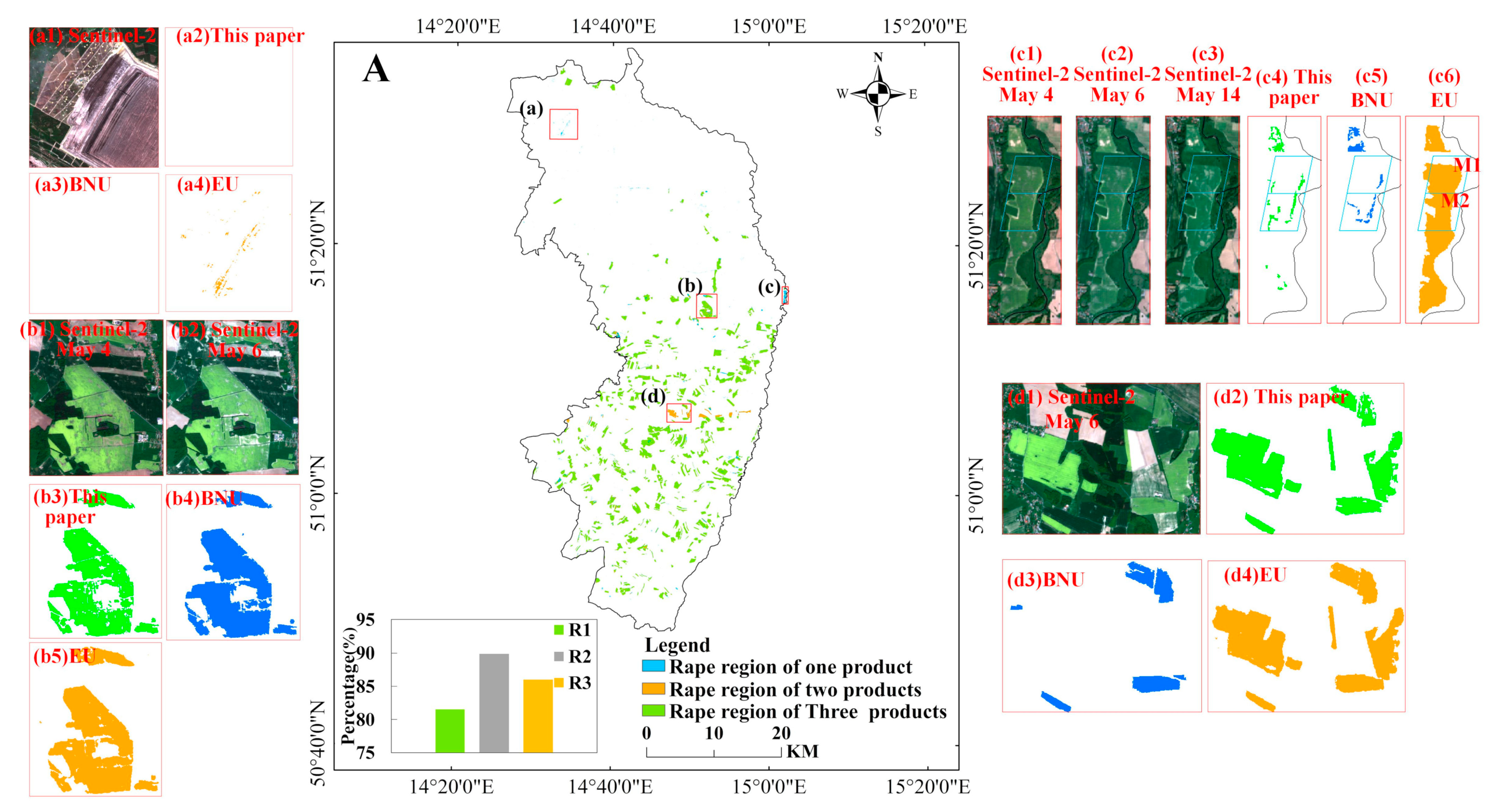

Table 1.
Type and quantity of the data in the spectral library.
| Spectral Library | Feature Type—Broad Categories | Feature Type—Subcategory | Spectrometer | Spectrum Number |
|---|---|---|---|---|
| Aster | Soil | Black loam, brown fine sandy loam, grayish brown loam, light yellowish-brown clay, brown to dark brown gravelly fine sandy loam, etc. | Becknic | 41 |
| Water Body | Ice, fine snow, medium granular snow, coarse granular snow, frost, tap water | Becknic | 6 | |
| USGS | Green Vegetation | Fir, whitebark, cactus, geranium, pansy, petunia, aspen, lichen, etc. | ASD | 41 |
| AVIRIS | 39 | |||
| Veg (ENVI) | Green Vegetation | Bay laurel, red willow, coast redwood, etc. | Beckman | 16 |
| Total | 143 | |||
Table 2.
Accuracy evaluation of rape in Görlitz, 2018.
| Rape | Non-Rape | User Accuracy | |
|---|---|---|---|
| Rape | 67 | 3 | 95.71 |
| Non-Rape | 2 | 128 | 98.46 |
| Producer Accuracy | 97.1 | 97.71 | |
| Overall Accuracy = 97.5%, Kappa coefficient = 0.94 | |||
Disclaimer/Publisher’s Note: The statements, opinions and data contained in all publications are solely those of the individual author(s) and contributor(s) and not of MDPI and/or the editor(s). MDPI and/or the editor(s) disclaim responsibility for any injury to people or property resulting from any ideas, methods, instructions or products referred to in the content. |
© 2023 by the authors. Licensee MDPI, Basel, Switzerland. This article is an open access article distributed under the terms and conditions of the Creative Commons Attribution (CC BY) license (https://creativecommons.org/licenses/by/4.0/).
Share and Cite
MDPI and ACS Style
Shao, C.; Shuai, Y.; Wu, H.; Deng, X.; Zhang, X.; Xu, A. Development of a Spectral Index for the Detection of Yellow-Flowering Vegetation. Remote Sens. 2023, 15, 1725. https://doi.org/10.3390/rs15071725
AMA Style
Shao C, Shuai Y, Wu H, Deng X, Zhang X, Xu A. Development of a Spectral Index for the Detection of Yellow-Flowering Vegetation. Remote Sensing. 2023; 15(7):1725. https://doi.org/10.3390/rs15071725
Chicago/Turabian StyleShao, Congying, Yanmin Shuai, Hao Wu, Xiaolian Deng, Xuecong Zhang, and Aigong Xu. 2023. "Development of a Spectral Index for the Detection of Yellow-Flowering Vegetation" Remote Sensing 15, no. 7: 1725. https://doi.org/10.3390/rs15071725
Note that from the first issue of 2016, this journal uses article numbers instead of page numbers. See further details here.