
A Hybrid ENSO Prediction System Based on the FIO−CPS and XGBoost Algorithm
by
 ,
,
Zhiyuan Kuang
1,2,
Yajuan Song
1,2,
Jie Wu
3,
Qiuying Fu
1,2,
Qi Shu
1,2,
Fangli Qiao
1,2 and
Zhenya Song
1,2,* 1
First Institute of Oceanography, and Key Laboratory of Marine Science and Numerical Modeling, Ministry of Natural Resources, Qingdao 266061, China
2
Shandong Key Laboratory of Marine Science and Numerical Modeling, Qingdao 266061, China
3
China Meteorological Administration Key Laboratory for Climate Prediction Studies, National Climate Center, Beijing 100081, China
*
Author to whom correspondence should be addressed.
Remote Sens. 2023, 15(7), 1728; https://doi.org/10.3390/rs15071728
Submission received: 20 February 2023
/
Revised: 20 March 2023
/
Accepted: 21 March 2023
/
Published: 23 March 2023
(This article belongs to the Special Issue Applications of Remote Sensing in Oceanography: Prospects and Challenges II)
Abstract
:Accurate prediction of the El Niño–Southern Oscillation (ENSO) is crucial for climate change research and disaster prevention and mitigation. In recent decades, the prediction skill for ENSO has improved significantly; however, accurate forecasting at a lead time of more than six months remains challenging. By using a machine learning method called eXtreme Gradient Boosting (XGBoost), we corrected the ENSO predicted results from the First Institute of Oceanography Climate Prediction System version 2.0 (FIO−CPS v2.0) based on the satellite remote sensing sea surface temperature data, and then developed a dynamic and statistical hybrid prediction model, named FIO−CPS−HY. The latest 15 years (2007–2021) of independent testing results showed that the average anomaly correlation coefficient (ACC) and root mean square error (RMSE) of the Niño3.4 index from FIO−CPS v2.0 to FIO−CPS−HY for 7− to 13−month lead times could be increased by 57.80% (from 0.40 to 0.63) and reduced by 24.79% (from 0.86 °C to 0.65 °C), respectively. The real−time predictions from FIO−CPS−HY indicated that the sea surface state of the Niño3.4 area would likely be in neutral conditions in 2023. Although FIO−CPS−HY still has some biases in real−time prediction, this study provides possible ideas and methods to enhance short−term climate prediction ability and shows the potential of integration between machine learning and numerical models in climate research and applications.
1. Introduction
The El Niño–Southern Oscillation (ENSO) is the strongest signal of interannual variability in the coupled ocean–atmosphere system [1,2]; it not only significantly affects tropical climate and weather, but also influences extratropical areas through processes such as atmospheric teleconnection and ocean circulation [1,3,4,5,6]. These processes subsequently affect global terrestrial and marine ecosystems [7,8,9], as well as agricultural production and food security [10,11]. Therefore, accurate ENSO prediction is not only important for short−term climate prediction studies, but also crucial for disaster prevention and mitigation [12,13].
ENSO prediction has been extensively examined over the past four decades [6,13,14,15]. Traditionally, the tools for ENSO prediction can be divided into statistical and dynamical models. Statistical models are mainly based on using historical data to find the relationship between ENSO and predictors. These models include multiple linear regression, principal oscillation pattern [16], analog analysis [17], canonical correlation analysis [18,19], climatology and persistence modeling [20], singular spectrum analysis [21], Markov modeling [22], and linear inverse modeling [23]. Current statistical models can achieve an anomaly correlation coefficient (ACC) greater than 0.7 for the Niño3.4 index at a 6−month lead time [24]. These statistical models have played a steady role in ENSO predictions with the advantages of lower computational cost and ease of operation [25].
Dynamical prediction models are based on numerical models that describe changes in the ocean–atmosphere and their interactions to achieve ENSO predictions. Since the first air–sea coupled ENSO prediction model was established [26,27], these models have been improved significantly. There are three main types of dynamical prediction models, namely simple air–sea coupled models [28], intermediate coupled models [29], and coupled general circulation models or climate models [15,30]. With increasing knowledge of physical processes, development of assimilation prediction technology, and increase in available satellite observation data, the prediction skill of dynamical models for ENSO has realized significant progress [31,32], and the dynamical model has currently become the most important ENSO prediction tool [13]. Currently, there are numerous institutes that perform real−time ENSO predictions, such as the International Research Institute for Climate and Society (IRI) at Columbia University, the European Centre for Medium−Range Weather Forecasts (ECMWF), and the Beijing Climate Center of China. The IRI released the multi−model mean predictions’ ACC of the monthly Niño3.4 index (https://iri.columbia.edu/our−expertise/climate/forecasts/enso/current/#, accessed on 20 March 2023.), which can be greater than 0.8 and near 0.6 at 6− and 12−month lead times, respectively [33,34]. The skill of the latest generation prediction system, Seasonal Forecasting System 5 (SEAS5), developed by ECMWF, can exceed 0.85 at a 6−month lead time [35]. The China multi−model ensemble prediction system (CMME) provides monthly releases of ENSO real−time predictions (http://ncclcs.ncc−cma.net/Website/index.php?ChannelID=254&WCHID=252, accessed on 20 March 2023), which shows that the multi−model mean prediction skill is over 0.8 at a 6−month lead time [36].
Although current models have achieved significant progress in ENSO prediction, there are still many challenges. For example, the prediction skill at one−year lead times is still relatively low, and the ACC values of many models are still below 0.6 [33,34,37]. This indicates that the model cannot provide effective predictions. The spread of the prediction results from multiple models is large, which yields significant prediction uncertainty [6,34,38]. Moreover, both dynamical and statistical models generally suffer from the spring predictability barrier (SPB) in ENSO prediction [15,39,40,41,42]. In addition, some researchers have found that the prediction skill after 2000 is much lower than during 1982−2000 by using multi−model ensemble hindcasts [43,44,45]. All of these challenges severely limit a longer and more accurate ENSO prediction.
In recent years, a new type of statistical method represented by machine learning, also including deep learning, has shown significant potential in geoscience applications [46,47,48,49]. Relevant research on ENSO predictions has been performed via two main methods: data−driven direct prediction and model result correction [37,50,51,52,53]. In terms of direct prediction, Ham et al. [37] combined convolutional neural networks (CNNs) and transfer learning to predict ENSO at long lead times. Based on 100−year−long SST observations and CMIP5 climate model data, they achieved the first breakthrough in an ENSO prediction skill over 0.5 at a 17−month lead time. Zhou and Zhang [54] combined the principal oscillation pattern (POP) method with a CNN−LSTM network to develop a POP−Net ENSO prediction model with a prediction skill over 0.5 at a 17−month lead time. Patil et al. [55] predicted ENSO using CNNs based on more than 100 years of observed SST anomalies and vertically averaged SST anomalies. Their results show a skillful prediction for long lead times (18− to 23−month lead times) and over 0.62 in January at an 18−month lead time. In terms of model result correction, most studies have focused on multi−model ensemble results. For example, Zhang et al. [50] used the Bayesian model averaging method to perform corrections on multiple statistical and dynamical model results. They showed that the corrected prediction skill was higher than any single model value. Li [56] utilized multiple decision tree algorithms to correct the multi−model prediction results; the prediction skill was equal to or higher than the results of the dynamical and statistical models. Furthermore, Li concluded that selecting dynamical and statistical model results as input features is more important for short and long lead times, respectively. All of these studies indicate the powerful role and fairly good application prospects of machine learning in ENSO prediction. However, these studies are based on multi−model ensemble results, and correcting short−term climate predictions based on single model predictions remains challenging due to insufficient data.
Recently, the First Institute of Oceanography, Ministry of Natural Resources developed the second−generation short−term climate prediction system FIO−CPS v2.0 (First Institute of Oceanography Climate Prediction System version 2.0), which is based on the developed coupled wave Earth system model, FIO−ESM v2.0 [30,57]. Although the ENSO hindcast skill of FIO−CPS v2.0 exceeds 0.75 at a 6−month lead time, the value of the ACC decreases to 0.45 at a 12−month lead time. Furthermore, as previously mentioned, the prediction skill of FIO−CPS v2.0 during 2002−2021 is significantly lower than that during 1982−2001. Meanwhile, the SPB phenomenon still exists in ENSO predictions. To improve the ENSO prediction skills of FIO−CPS v2.0, we attempt to utilize machine learning to correct the hindcast results based on FIO−CPS v2.0 dynamical predictions, design a hybrid prediction model with FIO−CPS v2.0 and machine learning, referred to as FIO−CPS−HY, and then verify its correction skills.
The remainder of this paper is organized as follows. Section 2 introduces the method, data, and idea of correcting the results of FIO−CPS v2.0. Section 3 evaluates the corrected results based on FIO−CPS−HY. Section 4 discusses FIO−CPS−HY input features and the impact of observation data on the prediction results. Finally, Section 5 summarizes the results and provides real−time ENSO prediction.
2. Datasets and Methods
2.1. FIO−CPS v2.0 Bias Correction Ideas
The predicted bias of FIO−CPS v2.0 has two main sources: initial bias due to data assimilation [58,59] and model bias due to various assumptions and approximations introduced by the imperfect description of dynamical processes and parameterization schemes [60,61], also known as intrinsic bias. We considered both the initial and intrinsic biases and corrected predicted SST anomalies over the Niño3.4 area using the machine learning model.
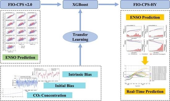
Figure 1 shows a schematic diagram of the ENSO hybrid prediction model, FIO−CPS−HY (First Institute of Oceanography Climate Prediction System Hybrid), based on FIO−CPS v2.0 and machine learning. FIO−CPS−HY first characterizes the intrinsic bias (CO2 concentration introduced to highlight the effect of external forcing) and initial bias of FIO−CPS v2.0. It obtains a time series of the intrinsic bias anomaly, the initial bias anomaly of FIO−CPS v2.0, and the global mean CO2 concentration anomaly. Then, the two sources of biases are combined with the prediction dimension of FIO−CPS v2.0 and adapted to 1− to 13−month lead times using transfer learning [62] to correct the original hindcast SST anomaly. Finally, the corrected SST anomaly and Niño3.4 index can be obtained. Specifically, for the intrinsic bias of FIO−CPS v2.0, the original biases of the SST in the FIO−ESM v2.0 historical simulation and future scenario experiment, i.e., SSP2−4.5, are used to characterize the intrinsic bias of the model (in FIO−CPS v2.0, external forcing data, including solar radiation, CO2 concentration, and other forcing data after 2015, were employed for the future scenario projection data of SSP2−4.5). The XGBoost (eXtreme Gradient Boosting) model in machine learning is used to predict and obtain the final intrinsic bias. We then adapt the bias values required for the target months of the FIO−CPS v2.0 hindcast and real−time predictions. The global mean CO2 concentration required by FIO−ESM v2.0 is directly adapted to the target month of FIO−CPS v2.0. For the initial bias, the SST of the assimilation outputs is compared with the observations to characterize the initial bias. As the prediction system corresponds to the same initial field before predicting from the same month, the initial bias anomaly is relatively small and constant. Thus, the assimilated bias anomaly is adapted as the initial bias of the 13 target months starting from the same month. Finally, based on the two adapted sources of biases and the original SST anomaly predicted by FIO−CPS v2.0, a hybrid prediction model is developed to improve ENSO predictions.
2.2. Datasets
The data used in this study included observation data, FIO−ESM v2.0 simulations and projections, CO2 concentrations, and assimilation and prediction data from FIO−CPS v2.0 (Table 1). The observation data include (1) the fifth−generation Extended Reconstructed Sea Surface Temperature (ERSST v5) monthly results provided by the U.S. Oceanic and Atmospheric Administration (NOAA), with a horizontal resolution of 2° × 2° and monthly temporal resolution, spanning from 01/1854 to 01/2023 [63]. As the observational period is relatively long, we used it for intrinsic bias prediction in the prediction system. The observation data also include (2) daily results from the Optimum Interpolation Sea Surface Temperature (OISST v2.1) provided by NOAA, which incorporates satellites and other different platforms (ships, buoys, and Argo floats), with a horizontal resolution of 0.25° × 0.25° and a daily temporal resolution, spanning from 12/01/1981 to 12/31/2022 [64]. We first converted the OISST data into monthly average data. They then could be used for the initial bias calculation and transfer correction in FIO−CPS v2.0.
The SSTs from FIO−ESM v2.0 in historical simulation and SSP2−4.5 projection experiments were used. We selected the first set of experiments, i.e., r1i1p1f1, which was used to develop the short−term climate prediction system, FIO−CPS v2.0, in combination with assimilation prediction technology, with a horizontal resolution of 1.1° × (0.27–0.54°) and a monthly temporal resolution. We chose them during 01/1854−01/2023, with the historical simulated SST from 01/1854 to 12/2014 and SSP2−4.5 projected SST from 01/2015 to 01/2023. Additionally, the global mean CO2 concentration data were provided by CMIP6 (Coupled Model Intercomparison Project phase 6).
The assimilated results of the SST, also known as the initial field of the FIO−CPS v2.0, have the same horizontal and temporal resolution for the SSTs in FIO−ESM v2.0; the time span was 1 month in advance of the starting time of FIO−CPS v2.0 for predictions, from 12/1981 to 11/2021, including 480 months. The prediction data were the historical hindcast Niño3.4 SST from FIO−CPS v2.0 with 10 ensemble members. Here, we calculated the ensemble mean results as the prediction values. The starting prediction period of the hindcast experiment was from 01/1982 to 12/2021. We selected the prediction results for the subsequent 13 lead months for the starting prediction for each, such that the sample size was 480 for each lead month.
We adopted the Niño3.4 index to characterize the ENSO. The SST anomaly, two sources of biases’ anomaly, and global mean CO2 concentration anomaly were calculated with respect to their respective climatology in 1991–2020. We obtained the Niño3.4 index from the three−month running mean value of the SST anomaly [65].
2.3. Machine Learning Model
XGBoost (Extreme Gradient Boosting) is an integrated machine learning algorithm based on a gradient boosting regression tree (GBDT), which integrates many weaker learners to form a strong learner [66].
XGBoost is an additive model consisting of base models, assuming that the tree model for sample i, , to be trained in the t−th iteration is written as follows:
wheredenotes the prediction result of sample i after the t−th iteration, denotes the prediction result of the previous t – 1 trees, and denotes the model of sample i in the t−th tree. The objective function is defined as follows:
where is the training loss for all samples, and is the complexity summation of all t trees, added to the objective function as a regularization term to prevent overfitting of the model. The objective function is expanded by a second−order Taylor series at and simplified to obtain the final objective function as follows:
where and are the first− and second−order derivatives of the loss function, respectively. Only and at each step are required; then, the objective function is optimized to obtain at each step. Finally, an overall model is obtained according to the additive model.
XGBoost has achieved strong power in major machine learning competitions [67] and has emerged in several applications in geosciences [68,69,70], especially climate prediction. For example, Zhang et al. developed a new model to predict droughts using a past drought index, meteorological measures, and climate signals from 32 stations from 1961 to 2016 in Shaanxi province, China. They selected three machine learning models including XGBoost and compared their validations for predicting the Standardized Precipitation Evapotranspiration Index (SPEI) 1–6 months in advance, and the XGBoost model more accurately predicted SPEI with a lead time of 1–6 months than other models [71]. Qian et al. developed three models including XGBoost to perform seasonal forecasts of the surface air temperature in winter in North America, and the XGBoost model hindcasts showed better forecast performances [72]. Huang et al. constructed 12 machine learning models to predict and compare daily and monthly values of solar radiation, and a stacking model using the best of these algorithms was developed to predict solar radiation. They concluded that the stacking model and the XGBoost model are the best models for predicting solar radiation [73]. Yang et al. applied many machine learning models to predict wave energy flux in the 31 geographical coordinate points in the Bohai sea separately, based on the data of the mean wave period, the significant wave height, and water depth. Their results showed that the gradient boosting machine, XGBoost, and stacked ensemble models yielded the best performance out of all algorithms [74].
Compared to the deep learning model (e.g. CNN), XGBoost can better process table data, and has stronger interpretability. In addition, it has merits such as easy parameter tuning, input data invariance, reliability, flexibility, and accuracy in many cases. And the actual performance of XGBoost is top notch in most regression and classification issues. Therefore, considering the sample size of the short−term climate prediction system is only 40 years in this study, a machine learning model that requires small training datasets is preferred over complex deep learning. Therefore, we selected XGBoost to conduct ENSO correction experiments.
2.4. Evaluation Metrics
Two statistical metrics, RMSE and ACC, were used to evaluate the mean bias and linear correlation between the prediction and observation, expressed as follows:
where represents the sample size; and represent the Niño3.4 index predicted and observed in the t−th month, respectively; and and represent the mean of the prediction and observation in months, respectively.
2.5. FIO−CPS−HY’s Establishment
2.5.1. Intrinsic Bias Prediction
The XGBoost model was used to train and predict the intrinsic bias of the prediction system based on the outputs of historical simulations and future scenario experimental results from FIO−ESM v2.0. According to the scatter diagram of the SST and SST bias from the FIO−ESM v2.0 simulations and projections (Figure 2), along with the increase in the FIO−ESM v2.0 SST, the SST bias also gradually changed from negative to positive, which initially reflected a basic linear relationship between the two. Therefore, based on the FIO−ESM v2.0 SST as input, the global mean CO2 concentration, important external forcing data affecting SST variation, was additionally introduced as a feature to achieve a more accurate regression prediction of the intrinsic bias.
In the XGBoost model, the real intrinsic bias (i.e., the bias of FIO−ESM v2.0) was regarded as ground truth. The input was the FIO−ESM v2.0 SST and global mean CO2 concentration during the same month. The output was the predicted intrinsic bias of the given month. The dataset was randomly divided into a training set (including 1669 months) and a test set (including 360 months). In the training process in XGBoost, the GridSearch method based on 5−fold cross−validation was for tuning the model parameters. We mainly tuned nine parameters of XGBoost. Among them, n_estimators is the number of weak evaluators, and the larger the value of n_estimators, the stronger the learning ability of the model, but the easier the overfitting of the model; learn_rate is the step size of training the model, and when iterating the decision tree, it controls the iteration rate to prevent overfitting; max_depth is the maximum depth of the tree, and increasing its value will make the model stronger but more likely to overfit; min_child_weight is the minimum sample weight required on a leaf node, and when the value is large, it can prevent the model from learning local special samples to prevent the model from overfitting; gamma is the penalty term of model complexity, and the larger the value, the more conservative the algorithm will be; subsample and colsample_bytree can control the proportion of samples taken from the training data; and reg_alpha and reg_lambda are regularization penalty coefficients and can reduce model complexity.
The final model parameters are as follows: n_estimators = 500, learn_rate = 0.1, max_depth = 24, min_child_weight = 5, gamma = 0.1, subsample = 0.6, colsample_bytree = 0.6, reg_alpha = 0.01, and reg_lambda = 2.
As listed in Table 2, the RMSE values of the predicted and real intrinsic bias for the training set, test set, and hindcast results (01/1982 to 12/2022) were all less than 0.39 °C, and correlation coefficient (CC) values were all above 0.96. Specifically, the RMSE of the hindcast results for subsequent FIO−CPS v2.0 SST correction was less than 0.21 °C, and the CC value exceeded 0.99. The time series of the real and predicted intrinsic bias for the hindcast period also indicate that the results of XGBoost fit the real intrinsic bias well (Figure 3), such that the predicted results were used as the intrinsic bias component of the subsequent transfer correction.
2.5.2. Initial Bias
The time series of the initial bias from FIO−CPS v2.0 was calculated as the difference between the assimilation SST and OISST, as shown in Figure 4. These values were all between −1 °C and 1 °C after assimilation, substantially reduced compared with the intrinsic bias (Figure 3). However, the initial bias was still not negligible. It was used as the initial bias of the subsequent transfer correction.
2.5.3. Transfer Correction of FIO−CPS v2.0
Based on the above analysis, we obtained the predicted intrinsic bias of FIO−CPS v2.0 based on the simulated and projected SST bias from FIO−ESM v2.0. In essence, the similarity between FIO−ESM v2.0 and FIO−CPS v2.0 is similar to the sample−based transfer in transfer learning. Therefore, the initial bias anomaly of FIO−CPS v2.0, predicted intrinsic bias anomaly, and global mean CO2 concentration anomaly values could be adapted to the predicted results of the prediction system. For the initial bias anomaly of the starting prediction month, it was adapted to 13 target months starting from that month. For example, the initial bias anomaly of 12/1981 was adapted to the results of the subsequent 13 months starting from 01/1982. In addition, the intrinsic bias anomaly and global mean CO2 concentration anomaly were directly adapted to the target month at the same time by the prediction system; e.g., the intrinsic bias anomaly and global mean CO2 concentration anomaly values in 12/1982 were directly adapted to the results of 12/1982 predicted by the prediction system for 13 different lead times.
We constructed XGBoost models of the transfer correction for 1− to 13−month lead times in order: XGBoost_1, XGBoost_2, ..., XGBoost_13. For each correction model, the ground truth was obtained from OISST. The input had four feature factors, including the original SST anomaly in the Niño3.4 region predicted by FIO−CPS v2.0 in the same month, intrinsic bias anomaly of the prediction system, anomaly of the global mean CO2 concentration, and initial bias anomaly of the prediction system. The output was the corrected prediction SST anomaly of each month. We divided the hindcast dataset in chronological order, with the training set’s prediction from 1982 to 2006 and the test set’s prediction from 2007 to 2021, such that we could independently evaluate the prediction skills of models in the later period. The parameter−tuning process also used the GridSearch method based on 5−fold cross−validation to optimize the parameters of each corrected model. Finally, 13 model parameter schemes were obtained.
The Niño3.4 index was calculated after applying the trained model to the test set results. A hybrid prediction model based on the combination of FIO−CPS v2.0 and XGBoost was established, denoted as FIO−CPS−HY.
3. Results
The prediction metrics (including RMSE and ACC) of FIO−CPS v2.0 and FIO−CPS−HY for the Niño3.4 index in the training set, test set, and entire hindcast period were evaluated (Figure 5 and Figure 6). The RMSE of FIO−CPS−HY in the training set had decreased to varying degrees for 13 lead times and obtained higher improvement for 7− to 13−month lead times. At a 13−month lead time, the RMSE of FIO−CPS−HY was 0.54 °C, which decreased by 26.47% compared with the values of 0.73 °C in FIO−CPS v2.0. The average RMSE for 7− to 13−month lead times from FIO−CPS v2.0 to FIO−CPS−HY could be reduced by 38.81% (from 0.63 °C to 0.38 °C) (see Figure 5a). Meanwhile, the ACC was more than 0.78 for all lead times. The improvement rate basically increased with the lead times; at 13−month lead times, the ACC of FIO−CPS−HY was 0.79, which increased by 41.76% compared with the values of 0.56 in FIO−CPS v2.0. An average ACC from FIO−CPS v2.0 to FIO−CPS−HY for 7− to 13−month lead times could be increased by 29.39% (from 0.69 to 0.90) (see Figure 5c). This shows that the hybrid prediction models were effectively trained.
As the independent period, the prediction skill of the test set is crucial to evaluate the generalization ability of our hybrid model. Except for the slightly worse than FIO−CPS v2.0 values (lower than 3.70%) at 2− to 3−month lead times, the RMSE from FIO−CPS v2.0 to FIO−CPS−HY has decreased. At a 13−month lead time, the RMSE decreased by 32.19% (from 0.95 °C to 0.64 °C), and the average RMSE for 7− to 13−month lead times could be reduced by 24.79% (from 0.86 °C to 0.65 °C) (see Figure 5b). For ACC results of FIO−CPS−HY, the improvement rate significantly increased with the lead times; an average ACC from FIO−CPS v2.0 to FIO−CPS−HY for 7− to 13−month lead times could be increased by 57.80% (from 0.40 to 0.63) (see Figure 5d). Representing an increase of more than 163.85%, the value of ACC reached more than 0.63 from 0.24 at a 13−month lead time. Furthermore, it is noteworthy that the prediction skills of FIO−CPS v2.0 in the test set were much worse than those in the training set, but the corrected results of FIO−CPS−HY have been able almost to approach and even exceed those of the earlier training period, especially for 12−to 13−month lead times.
Figure 5.
RMSE and ACC of the Niño3.4 index in FIO−CPS v2.0 and FIO−CPS−HY among the OISST, training set, and test set prediction results. (a) RMSE in the training set, (b) RMSE in the test set, (c) ACC in the training set, and (d) ACC in the test set. The blue and red lines represent the RMSE and ACC of FIO−CPS v2.0 and FIO−CPS−HY for 1− to 13−month lead times, respectively. The red bar represents the percent improvement in FIO−CPS−HY relative to FIO−CPS v2.0, calculated via the absolute difference between two models divided by the RMSE or ACC of FIO−CPS v2.0 (units: %).

Here, we could obtain the whole hindcast Niño3.4 index time series, and the difference in prediction skill between FIO−CPS v2.0 and FIO−CPS−HY is shown in Figure 6. The hindcast period (prediction from 01/1982 to 12/2021) shows that the RMSE of FIO−CPS−HY decreased to within 0.58 °C from 0.82 °C and decreased by 29.29% at the 13−month lead time, with the average RMSE for 7− to 13−month lead times could be reduced by 30.28% (from 0. 73 °C to 0.51 °C) (see Figure 6a). The ACC increased to more than 0.73 from 0.41, increasing by 79.15%; even an average ACC from FIO−CPS v2.0 to FIO−CPS−HY for 7− to 13−month lead times could be increased by 45.96% (from 0.55 to 0.81) (see Figure 6b). So, the hindcast results of FIO−CPS−HY could provide higher−quality data for the subsequent ENSO prediction research.
Figure 6.
RMSE and ACC of the Niño3.4 index in FIO−CPS v2.0 and FIO−CPS−HY between the OISST and the whole hindcast results (prediction from 01/1982 to 12/2021). (a) RMSE and (b) ACC. The blue and red lines represent the results of FIO−CPS v2.0 and FIO−CPS−HY, respectively. The red bar represents the percent improvement by FIO−CPS−HY relative to FIO−CPS v2.0, calculated via the absolute difference between the two models divided by the RMSE or ACC of FIO−CPS v2.0.

Figure 7 shows the RMSE and ACC of the Niño3.4 index of FIO−CPS v2.0 and FIO−CPS−HY as a function of the predicted target month and lead time in the test set. Compared with FIO−CPS v2.0, the prediction skills of FIO−CPS−HY significantly improved, especially in boreal summer and autumn. The significant positive difference in the ACC as the target month ranged from July to November indicates that the predictability in summer and autumn has been improved in FIO−CPS−HY (see Figure 7f). Furthermore, we found that the longer the lead times, the greater the improvement rate of FIO−CPS−HY; the ACC has increased by more than 0.46 in summer and more than 0.14 for other target months from 11−month lead times. Meanwhile, it was obvious that the SPB phenomenon has been alleviated more with the extension of lead times. In addition, the pattern of the RMSE reduction was basically similar to the pattern of the ACC improvement; the RMSE had a much sharper decline with longer lead times, decreasing by 0.21 °C from 11−month lead times (see Figure 7e). In general, FIO−CPS−HY produced a better ENSO predictability, especially in boreal summer and autumn; although SPB still existed both in FIO−CPS v2.0 and FIO−CPS−HY, FIO−CPS−HY improved it clearly and had a better persistence.
To explore the improvement of FIO−CPS−HY in more detail, the scatter diagrams of the Niño3.4 index for all lead months in the test set based on the FIO−CPS v2.0 and FIO−CPS−HY outputs are shown in Figure 8. We found that the spatial contour of scatters of FIO−CPS−HY was clearly smaller than that of FIO−CPS v2.0, especially for 8−month to 13−month lead times, and the scatterplot’s center was closer to the diagonal. Although we also noted that the corrected results of FIO−CPS−HY had a relatively poor effect on values of FIO−CPS v2.0 that are too low relative to OISST, most of the corrections were closer to the observation for longer lead times.
4. Discussion
Although the FIO−CPS−HY hybrid prediction model improved the prediction ability for ENSO, three issues require further discussion: (1) What are the effects of different input features in the correction model on the correction results? In other words, this is the issue of feature importance. (2) OISST was used for the initial bias and correction model of the prediction system while ERSST was used for the intrinsic bias prediction model. To what extent do the observation data, with different types and lengths, affect the correction results? In other words, this is the issue of the selection of training observation data. (3) The prediction skill of FIO−CPS−HY significantly increases for 7− to 13−month lead times. However, the increase in the prediction skill of FIO−CPS−HY is relatively smaller for 1− to 6−month lead times. The reasons need to be discussed. Based on these three issues, we provide further discussion.
4.1. Feature Importance
Feature importance is a measure of the magnitude of each feature input in a decision tree model. The greater the performance of a feature for decision tree split point improvement, the greater the importance of that feature. The importance values of the output feature are shown in Figure 9. We found that the hindcast SST anomaly of FIO−CPS v2.0 was the most important for 1− to 9−month lead times, with values all above 0.4, and the values also exceeded 0.3 from 10−month lead time. This is because our correction task was based on the hindcast SST anomaly results of FIO−CPS v2.0, followed by the introduction of other features. With the extension of the lead times, the importance of the hindcast SST anomaly gradually decreased; the sum of three other statistical features gradually increased (the sum of the values of the four important features is 1), especially for the intrinsic bias anomaly, which gradually increased with the lead time and was more than 0.4 from 10−month lead time. As proposed by Li [56], other statistical factors with a stronger correction role should be considered at long lead times. Meanwhile, the contribution of the global mean CO2 concentration also played a slightly larger role than the initial bias for most lead months. This implies that SST anomaly correction with an increase in the lead time requires intrinsic bias and external forcings. From here, we propose that improvements to the physical processes, parameterization schemes, and accuracy of the response to external forcings are necessary. The initial bias was the least important component for most lead times because the overall assimilated initial bias was substantially reduced compared to the intrinsic bias. It played a relatively small role in the correction models but still had a certain contribution.
4.2. Comparison of Observation Data
In this study, ERSST v5 during 01/1854–01/2023 was used to produce the intrinsic bias prediction and introduce this intrinsic bias into the final correction model. OISST v2.1 during 12/1981–12/2022 was used to calculate the initial bias and evaluate the prediction system. To show the impact of two different observations on the final correction results, three additional sets of intrinsic bias prediction experiments using different observations and four sets of correction experiments using different observations were designed for comparison with the existing experiment above. As listed in Table 3, a total of five experiments containing the initial bias, intrinsic bias, and transfer correction were designed based on the four intrinsic bias prediction experiments.
To evaluate the performances of different experiments at long lead times, we compare the average RMSE and ACC for 7− to 13−month lead times in Table 4. The results show that all the experiments’ RMSE and ACC changed across a small range. The maximum difference of the RMSE was within 0.05 °C, and the ACC was between 0.58 and 0.66. In addition to an experiment combination, i.e., Init_OI_198112 + Intri_OI_198201 + TC_OI_198201, with slightly poor prediction skills, other different observation data selections have a small impact on the hybrid prediction results, also reflecting the stability and robustness of our hybrid model. The ACC results of ERSST were the best observation for the initial bias, intrinsic bias, and prediction system, but the improvement was not significant compared with our existing experimental results. Meanwhile, the existing experiment has a minimum RMSE of only 0.65 °C. Considering that the OISST has been widely used in the evaluation of ENSO prediction skill [24,33,34], as well as integrated satellite data with higher spatial and temporal resolutions, we selected the existing experiment as the final result.
4.3. Prediction Skill of FIO−CPS−HY
From the results above, we can find that the prediction skill of FIO−CPS−HY significantly increases for 7− to 13−month lead times. However, the increase in the prediction skill of FIO−CPS−HY is relatively smaller for 1− to 6−month lead times. Some reasons need to be discussed.
As shown in Figure 5a,c, The RMSE and ACC in the training set for 1− to 6−month lead times from FIO−CPS v2.0 showed good prediction performance. The average RMSE and ACC for 1− to 6−month lead times from FIO−CPS v2.0 was less than 0.40 °C and more than 0.88. Therefore, it is easy to understand that the statistics’ improvement for 1− to 6−month lead times from FIO−CPS v2.0 to FIO−CPS−HY was relatively small. The prediction error increases with the increase in lead time; in order to reveal the error characteristic changes in FIO−CPS v2.0 in more detail, Figure 10 shows the scatter diagrams of the Niño3.4 index for all lead months in the training set based on the FIO−CPS v2.0 and FIO−CPS−HY outputs. It is clear that the scatter points gradually deviate from the diagonal with the increase in lead time. Meanwhile, when we conducted ENSO correction experiments for 13 lead months separately, we adopted the same parameter range as large as possible to tune parameters, so as to ensure the fairness of parameter tuning and avoid the individual influence of different parameter−tuning schemes on the results of one model. Therefore, FIO−CPS−HY has more room for correction to achieve better results, on the premise of distribution characteristics with larger deviations in longer lead months.
As mentioned above, the ENSO prediction skill after 2000 is much lower than before. The average RMSE and ACC for 1− to 6−month lead times from FIO−CPS v2.0 were less than 0.46 °C and more than 0.80 (see Figure 5b,d). Following the rules of the training set, it seems that FIO−CPS−HY should have more room for correction in the test set. However, the scatter point data distribution characteristics of the test set have changed compared with the training set (see Figure 8). The coefficient of the best−fit linear regression line of FIO−CPS v2.0 became smaller, and the overall rotation was clockwise compared with the training set, which makes it harder for FIO−CPS−HY to correct FIO−CPS v2.0 values near the diagonal, especially on values of FIO−CPS v2.0 too low for OISST. Therefore, the statistics’ improvement for 1− to 6−month lead times from FIO−CPS v2.0 to FIO−CPS−HY was smaller than that for the training set. For 7− to 13−month lead times, the scatter point data distribution characteristics of the test set changed significantly compared with the training set, and the coefficient of the best−fit linear regression line of FIO−CPS v2.0 became much smaller. However, most of the scatter points are distributed in places where the value of FIO−CPS v2.0 is too high for OISST, which gives FIO−CPS−HY more room to correct the large deviation. This is the reason why the prediction skill of FIO−CPS−HY significantly increases for 7− to 13−month lead times.
In summary, the scatterplot distribution characteristics’ changes for FIO−CPS v2.0 and OISST make it easier for FIO−CPS−HY to correct the results for 7− to 13−month lead times but more difficult for FIO−CPS−HY to correct the results for 1− to 6−month lead times. This reflects that the prediction skills and bias characteristics of FIO−CPS v2.0 have changed in the recent 20 years, which suggests that we should strive to improve the prediction skills and carry out further dynamical model bias analysis and research in the future.
5. Conclusions
Based on the latest generation of the FIO−CPS v2.0 short−term climate prediction system and the XGBoost machine learning method, the hybrid prediction model FIO−CPS−HY was developed for ENSO prediction. Considering the initial bias and intrinsic bias of ENSO predictions, FIO−CPS−HY could find the nonlinear relationship among the FIO−CPS v2.0 hindcast SST, two−part bias, and observation while correcting the prediction results of the dynamical model.
The prediction skill of the Niño3.4 index in 2007–2021 significantly improved for 7− to 13−month lead times. The average ACC and RMSE from FIO−CPS v2.0 to FIO−CPS−HY for 7− to 13−month lead times could be increased by 57.80% (from 0.40 to 0.63) and reduced by 24.79% (from 0.86 °C to 0.65 °C). At the same time, a spring predictability barrier exists in FIO−CPS v2.0 and FIO−CPS−HY, but this problem is less pronounced in FIO−CPS−HY. Moreover, the prediction skill of FIO−CPS−HY significantly increases in boreal summer and autumn from 11−month lead times.
Based on the FIO−CPS−HY, we present the corrected results of the Niño3.4 index predicted from 09/2022 to 02/2023 in Figure 11. The latest 6 months’ predictions of FIO−CPS−HY show that the Niño3.4 index has dropped to a certain extent compared with FIO−CPS v2.0 and will be most likely to increase until March–April–May 2023 and then decrease. In general, the real−time predictions from FIO−CPS−HY indicate that the sea surface state of the Niño3.4 area would likely be in neutral conditions in 2023.
Author Contributions
Conceptualization, Z.S. and F.Q.; data curation, Y.S.; funding acquisition, Z.S.; methodology, Z.K., Y.S., J.W. and Q.F.; software, Q.F.; supervision, Z.S.; validation, J.W. and Q.S.; visualization, Z.K. and Y.S.; writing—original draft, Z.K.; writing—review and editing, Y.S., J.W., Q.F., Q.S., Z.S. and F.Q. All authors have read and agreed to the published version of the manuscript.
Funding
This research was funded by the Marine S&T Fund of Shandong Province for Laoshan Laboratory (LSKJ202202100), the National Natural Science Foundation of China (Nos. 42022042, 41821004, 42175052, and U1806205), the China–Korea Cooperation Project on the Northwest Pacific Marine Ecosystem Simulation under Climate Change, and CAS Interdisciplinary Innovation Team (JCTD-2020-12).
Data Availability Statement
The OISST data used in this study are available at https://www.ncei.noaa.gov/products/optimum-interpolation-sst (accessed on 21 March 2023); the ERSST data are available at https://psl.noaa.gov/data/gridded/data.noaa.ersst.v5.html (accessed on 21 March 2023); the FIO−ESM v2.0 SST, FIO−CPS v2.0, and FIO−CPS−HY data are available at https://doi.org/10.6084/m9.figshare.21996254.v3 (accessed on 18 February 2023).
Acknowledgments
We acknowledge the two anonymous reviewers and the editor for their constructive comments and suggestions for improving the manuscript.
Conflicts of Interest
The authors declare no conflict of interest.
References
- Bjerknes, J. Atmospheric teleconnections from the equatorial Pacific. Mon. Weather Rev. 1969, 97, 163–172. [Google Scholar] [CrossRef]
- Wang, C.Z. Three-ocean interactions and climate variability: A review and perspective. Clim. Dyn. 2019, 53, 5119–5136. [Google Scholar] [CrossRef]
- Zhang, R.H.; Sumi, A.; Kimoto, M. Impact of El Niño on the East Asian monsoon a diagnostic study of the’86/87 and’91/92 events. J. Meteorol. Soc. Jpn. Ser. II 1996, 74, 49–62. [Google Scholar] [CrossRef]
- Chen, W. Impacts of El Niño and La Niña on the cycle of the East Asian winter and summer monsoon. Chin. J. Atmos. Sci.-Chin. Ed. 2002, 26, 609–623. [Google Scholar]
- Timmermann, A.; An, S.; Kug, J.; Jin, F.F.; Cai, W.J.; Capotondi, A.; Cobb, K.M.; Lengaigne, M.; McPhaden, M.J.; Stuecker, M.F. El Niño–southern oscillation complexity. Nature 2018, 559, 535–545. [Google Scholar] [CrossRef]
- Zhang, R.H.; Yu, Y.Q.; Song, Z.Y.; Ren, H.L.; Tang, Y.M.; Qiao, F.L.; Wu, T.W.; Gao, C.; Hu, J.Y.; Tian, F. A review of progress in coupled ocean-atmosphere model developments for ENSO studies in China. J. Oceanol. Limnol. 2020, 38, 930–961. [Google Scholar] [CrossRef]
- McPhaden, M.J.; Zebiak, S.E.; Glantz, M.H. ENSO as an integrating concept in earth science. Science 2006, 314, 1740–1745. [Google Scholar] [CrossRef]
- Kløve, B.; Ala-Aho, P.; Bertrand, G.; Gurdak, J.J.; Kupfersberger, H.; Kværner, J.; Muotka, T.; Mykrä, H.; Preda, E.; Rossi, P. Climate change impacts on groundwater and dependent ecosystems. J. Hydrol. 2014, 518, 250–266. [Google Scholar] [CrossRef]
- Yao, Y.; Wang, C.Z. Marine heatwaves and cold-spells in global coral reef zones. Prog. Oceanogr. 2022, 209, 102920. [Google Scholar] [CrossRef]
- Zhang, T.Y.; Zhu, J.; Yang, X.G.; Zhang, X. Y Correlation changes between rice yields in North and Northwest China and ENSO from 1960 to 2004. Agric. For. Meteorol. 2008, 148, 1021–1033. [Google Scholar] [CrossRef]
- Li, Y.Y.; Strapasson, A.; Rojas, O. Assessment of El Niño and La Niña impacts on China: Enhancing the early warning system on food and agriculture. Weather Clim. Extrem. 2020, 27, 100208. [Google Scholar] [CrossRef]
- Ren, H.L.; Jin, F.F.; Song, L.C.; Lu, B.; Tian, B.; Zuo, J.Q.; Liu, Y.; Wu, J.J.; Zhao, C.B.; Nie, Y. Prediction of primary climate variability modes at the Beijing Climate Center. J. Meteorol. Res. 2017, 31, 204–223. [Google Scholar] [CrossRef]
- Tang, Y.M.; Zhang, R.H.; Liu, T.; Duan, W.S.; Yang, D.J.; Zheng, F.; Ren, H.L.; Lian, T.; Gao, C.; Chen, D. Progress in ENSO prediction and predictability study. Natl. Sci. Rev. 2018, 5, 826–839. [Google Scholar] [CrossRef]
- Latif, M.; Anderson, D.; Barnett, T.; Cane, M.; Kleeman, R.; Leetmaa, A.; O’Brien, J.; Rosati, A.; Schneider, E. A review of the predictability and prediction of ENSO. J. Geophys. Res. Oceans 1998, 103, 14375–14393. [Google Scholar] [CrossRef]
- Ren, H.L.; Zheng, F.; Luo, J.J.; Wang, R.; Liu, M.H.; Zhang, W.J.; Zhou, T.J.; Zhou, G.Q. A review of research on tropical air-sea interaction, ENSO dynamics, and ENSO prediction in China. J. Meteorol. Res. 2020, 34, 43–62. [Google Scholar] [CrossRef]
- Xu, J.S. Analysis and Prediction of the El Niño Southern Oscillation Phenomenon Using Principal Oscillation Pattern Analysis. Ph.D. Thesis, University of Hamburg, Hamburg, Germany, 1990. [Google Scholar]
- Van den Dool, H. Searching for analogues, how long must we wait? Tellus A 1994, 46, 314–324. [Google Scholar] [CrossRef]
- Barnston, A.G.; Van den Dool, H.M.; Zebiak, S.E.; Barnett, T.P.; Ji, M.; Rodenhuis, D.R.; Cane, M.A.; Leetmaa, A.; Graham, N.E.; Ropelewski, C.R. Long-lead seasonal forecasts—Where do we stand? Bull. Am. Meteorol. Soc. 1994, 75, 2097–2114. [Google Scholar] [CrossRef]
- He, Y.X.; Barnston, A.G. Long-lead forecasts of seasonal precipitation in the tropical Pacific islands using CCA. J. Clim. 1996, 9, 2020–2035. [Google Scholar] [CrossRef]
- Knaff, J.A.; Landsea, C.W. An El Niño–Southern Oscillation climatology and persistence (CLIPER) forecasting scheme. Weather Forecast 1997, 12, 633–652. [Google Scholar] [CrossRef]
- Ding, Y.G.; Jiang, Z.H.; Zhu, Y.F. Experiment on short term climatic prediction to SSTA over the NINO oceanic region. J. Trop. Meteorol. 1998, 14, 289–296. [Google Scholar]
- Xue, Y.; Leetmaa, A. Forecasts of tropical Pacific SST and sea level using a Markov model. Geophys. Res. Lett. 2000, 27, 2701–2704. [Google Scholar] [CrossRef]
- Alexander, M.A.; Matrosova, L.; Penland, C.; Scott, J.D.; Chang, P. Forecasting Pacific SSTs: Linear inverse model predictions of the PDO. J. Clim. 2008, 21, 385–402. [Google Scholar] [CrossRef]
- Ren, H.L.; Zuo, J.Q.; Deng, Y. Statistical predictability of Nino indices for two types of ENSO. Clim. Dyn. 2019, 52, 5361–5382. [Google Scholar] [CrossRef]
- Clarke, A.J. El Nino Physics and El Nino Predictability. Ann. Rev. Mar. Sci. 2014, 6, 79–99. [Google Scholar] [CrossRef]
- Cane, M.A.; Zebiak, S.E.; Dolan, S.C. Experimental forecasts of EL Nino. Nature 1986, 321, 827–832. [Google Scholar] [CrossRef]
- Zebiak, S.E.; Cane, M.A. A model el niñ–southern oscillation. Mon. Weather Rev. 1987, 115, 2262–2278. [Google Scholar] [CrossRef]
- Chen, D.K.; Cane, M.A.; Kaplan, A.; Zebiak, S.E.; Huang, D.J. Predictability of El Niño over the past 148 years. Nature 2004, 428, 733–736. [Google Scholar] [CrossRef]
- Zheng, F.; Zhu, J. Improved ensemble-mean forecasting of ENSO events by a zero-mean stochastic error model of an intermediate coupled model. Clim. Dyn. 2016, 47, 3901–3915. [Google Scholar] [CrossRef]
- Song, Y.J.; Shu, Q.; Bao, Y.; Yang, X.D.; Song, Z.Y. The short-term climate prediction system FIO-CPS v2. 0 and its prediction skill in ENSO. Front. Earth Sci. 2021, 9, 759339. [Google Scholar] [CrossRef]
- Zheng, F.; Zhu, J.; Zhang, R.H.; Zhou, G.Q. Ensemble hindcasts of SST anomalies in the tropical Pacific using an intermediate coupled model. Geophys. Res. Lett. 2006, 33, L19604. [Google Scholar] [CrossRef]
- Zheng, F.; Zhu, J.; Zhang, R.H. Impact of altimetry data on ENSO ensemble initializations and predictions. Geophys. Res. Lett. 2007, 34, L13611. [Google Scholar] [CrossRef]
- Barnston, A.G.; Tippett, M.K.; L’Heureux, M.L.; Li, S.; DeWitt, D.G. Skill of real-time seasonal ENSO model predictions during 2002–11: Is our capability increasing? Bull. Am. Meteorol. Soc. 2012, 93, 631–651. [Google Scholar] [CrossRef]
- Barnston, A.G.; Tippett, M.K.; Ranganathan, M.; L’Heureux, M.L. Deterministic skill of ENSO predictions from the North American Multimodel Ensemble. Clim. Dyn. 2019, 53, 7215–7234. [Google Scholar] [CrossRef] [PubMed]
- Johnson, S.J.; Stockdale, T.N.; Ferranti, L.; Balmaseda, M.A.; Molteni, F.; Magnusson, L.; Tietsche, S.; Decremer, D.; Weisheimer, A.; Balsamo, G. SEAS5: The new ECMWF seasonal forecast system. Geosci. Model Dev. 2019, 12, 1087–1117. [Google Scholar] [CrossRef]
- Ren, H.L.; Wu, Y.J.; Bao, Q.; Ma, J.H.; Liu, C.Z.; Wan, J.H.; Li, Q.P.; Wu, X.F.; Liu, Y.; Tian, B. The China multi-model ensemble prediction system and its application to flood-season prediction in 2018. J. Meteorol. Res. 2019, 33, 540–552. [Google Scholar] [CrossRef]
- Ham, Y.G.; Kim, J.H.; Luo, J.J. Deep learning for multi-year ENSO forecasts. Nature 2019, 573, 568–572. [Google Scholar] [CrossRef]
- Tippett, M.K.; Ranganathan, M.; L’Heureux, M.; Barnston, A.G.; DelSole, T. Assessing probabilistic predictions of ENSO phase and intensity from the North American Multimodel Ensemble. Clim. Dyn. 2019, 53, 7497–7518. [Google Scholar] [CrossRef]
- Webster, P. The annual cycle and the predictability of the tropical coupled ocean-atmosphere system. Meteorol. Atmos. Phys. 1995, 56, 33–55. [Google Scholar] [CrossRef]
- McPhaden, M.J.; Santoso, A.; Cai, W.J. El Niño Southern Oscillation in a Changing Climate; John Wiley & Sons: Hoboken, NJ, USA, 2020; Volume 253. [Google Scholar]
- Mu, M.; Xu, H.; Duan, W.S. A kind of initial errors related to “spring predictability barrier” for El Niño events in Zebiak-Cane model. Geophys. Res. Lett. 2007, 34, L03709. [Google Scholar] [CrossRef]
- Duan, W.S.; Zhao, P.; Hu, J.Y.; Xu, H. The role of nonlinear forcing singular vector tendency error in causing the “spring predictability barrier” for ENSO. J. Meteorol. Res. 2016, 30, 853–866. [Google Scholar] [CrossRef]
- Zhang, S.W.; Wang, H.; Jiang, H.; Ma, W.T. Evaluation of ENSO prediction skill changes since 2000 based on multimodel hindcasts. Atmosphere 2021, 12, 365. [Google Scholar] [CrossRef]
- Zhang, W.; Chen, Q.L.; Zheng, F. Bias corrections of the heat flux damping process to improve the simulation of ENSO post-2000. Sci. Online Lett. Atmos. 2015, 11, 181–185. [Google Scholar] [CrossRef]
- Zheng, F.; Zhang, W.; Yu, J.; Chen, Q. A possible bias of simulating the post-2000 changing ENSO. Sci. Bull. 2015, 60, 1850–1857. [Google Scholar] [CrossRef]
- Reichstein, M.; Camps-Valls, G.; Stevens, B.; Jung, M.; Denzler, J.; Carvalhais, N. Deep learning and process understanding for data-driven Earth system science. Nature 2019, 566, 195–204. [Google Scholar] [CrossRef]
- Irrgang, C.; Boers, N.; Sonnewald, M.; Barnes, E.A.; Kadow, C.; Staneva, J.; Saynisch-Wagner, J. Towards neural Earth system modelling by integrating artificial intelligence in Earth system science. Nat. Mach. Intell. 2021, 3, 667–674. [Google Scholar] [CrossRef]
- Schneider, R.; Bonavita, M.; Geer, A.; Arcucci, R.; Dueben, P.; Vitolo, C.; Le Saux, B.; Demir, B.; Mathieu, P.-P. ESA-ECMWF Report on recent progress and research directions in machine learning for Earth System observation and prediction. NPJ Clim. Atmos. Sci. 2022, 5, 51. [Google Scholar] [CrossRef]
- Sun, Z.H.; Sandoval, L.; Crystal-Ornelas, R.; Mousavi, S.M.; Wang, J.B.; Lin, C.; Cristea, N.; Tong, D.; Carande, W.H.; Ma, X. A review of earth artificial intelligence. Comput. Geosci. 2022, 159, 105034. [Google Scholar] [CrossRef]
- Zhang, H.P.; Chu, P.S.; He, L.K.; Unger, D. Improving the CPC’s ENSO forecasts using Bayesian model averaging. Clim. Dyn. 2019, 53, 3373–3385. [Google Scholar] [CrossRef]
- Kim, J.; Kwon, M.; Kim, S.D.; Kug, J.S.; Ryu, J.G.; Kim, J. Spatiotemporal neural network with attention mechanism for El Niño forecasts. Sci. Rep. 2022, 12, 7204. [Google Scholar] [CrossRef]
- Song, Z.Y.; Liu, W.G.; Liu, X.; Liu, H.X.; Su, T.Y.; Yin, X.Q. Research Progress and Perspective of the Key Technologies for Ocean Numerical Model Driven by the Mass Data. Adv. Mar. Sci. 2019, 37, 161–170. [Google Scholar]
- Dong, C.M.; Xu, G.J.; Han, G.Q.; Brandon, J.B.; Xie, W.H.; Zhou, S.Y. Recent Developments in Artificial Intelligence in Oceanography. Ocean Land Atmos. Res. 2022, 2022, 9870950. [Google Scholar] [CrossRef]
- Zhou, L.; Zhang, R.H. A hybrid neural network model for ENSO prediction in combination with principal oscillation pattern analyses. Adv. Atmos. Sci. 2022, 39, 889–902. [Google Scholar] [CrossRef]
- Patil, K.; Doi, T.; Oettli, P.; Jayanthi, V.R.; Behera, S. Long Lead Predictions of ENSO Using Convolutional Neural Networks. In Proceedings of the AGU Fall Meeting Abstracts, A13I-08, New Orleans, LA, USA, 13–17 December 2021. [Google Scholar]
- Li, C.T. The application of machine learning in ENSO prediction consultation. Mar. Forecast 2022, 39, 91–103. [Google Scholar]
- Bao, Y.; Song, Z.Y.; Qiao, F.L. FIO-ESM version 2.0: Model description and evaluation. J. Geophys. Res. Oceans 2020, 125, e2019JC016036. [Google Scholar] [CrossRef]
- Xu, H.; Duan, W.S. What kind of initial errors cause the severest prediction uncertainty of El Nino in Zebiak-Cane model. Adv. Atmos. Sci. 2008, 25, 577–584. [Google Scholar] [CrossRef]
- Zheng, F.; Wang, H.; Zhu, J. ENSO ensemble prediction: Initial error perturbations vs. model error perturbations. Chin. Sci. Bull. 2009, 54, 2516–2523. [Google Scholar] [CrossRef]
- Yu, Y.; Mu, M.; Duan, W.S. Does model parameter error cause a significant “spring predictability barrier” for El Niño events in the Zebiak–Cane model? J. Clim. 2012, 25, 1263–1277. [Google Scholar] [CrossRef]
- Tao, L.J.; Gao, C.; Zhang, R.H. Model parameter-related optimal perturbations and their contributions to El Niño prediction errors. Clim. Dyn. 2019, 52, 1425–1441. [Google Scholar] [CrossRef]
- Pan, S.J.; Yang, Q. A survey on transfer learning. IEEE Trans. Knowl. Data Eng. 2010, 22, 1345–1359. [Google Scholar] [CrossRef]
- Huang, B.; Thorne, P.W.; Banzon, V.F.; Boyer, T.; Chepurin, G.; Lawrimore, J.H.; Menne, M.J.; Smith, T.M.; Vose, R.S.; Zhang, H.-M. Extended reconstructed sea surface temperature, version 5 (ERSSTv5): Upgrades, validations, and intercomparisons. J. Clim. 2017, 30, 8179–8205. [Google Scholar] [CrossRef]
- Reynolds, R.W.; Smith, T.M.; Liu, C.; Chelton, D.B.; Casey, K.S.; Schlax, M.G. Daily high-resolution-blended analyses for sea surface temperature. J. Clim. 2007, 20, 5473–5496. [Google Scholar] [CrossRef]
- Kousky, V.; Higgins, R. An alert classification system for monitoring and assessing the ENSO cycle. Weather Forecast 2007, 22, 353–371. [Google Scholar] [CrossRef]
- Chen, T.Q.; Guestrin, C. Xgboost: A scalable tree boosting system. In Proceedings of the 22nd ACM SIGKDD International Conference on Knowledge Discovery and Data Mining, San Francisco, CA, USA, 13–17 August 2016; pp. 785–794. [Google Scholar]
- Nielsen, D. Tree Boosting with xgboost-Why Does Xgboost Win “Every” Machine Learning Competition? NTNU: Trondheim, Norway, 2016. [Google Scholar]
- Liu, L.L.; Liu, H.C.; Zhu, C.F. Thunderstorm weather analysis based on XGBoost algorithm. Int. Arch. Photogramm. Remote Sens. Spat. Inf. Sci. 2020, 42, 261–264. [Google Scholar] [CrossRef]
- Feng, Y.L.; Gao, Z.; Xiao, H.; Yang, X.D.; Song, Z.Y. Predicting the Tropical Sea Surface Temperature Diurnal Cycle Amplitude Using an Improved XGBoost Algorithm. J. Mar. Sci. Eng. 2022, 10, 1686. [Google Scholar] [CrossRef]
- Liu, F.; Wang, X.M.; Sun, F.B.; Wang, H.; Wu, L.F.; Zhang, X.Z.; Liu, W.B.; Che, H.Z. Correction of Overestimation in Observed Land Surface Temperatures Based on Machine Learning Models. J. Clim. 2022, 35, 5359–5377. [Google Scholar] [CrossRef]
- Zhang, R.; Chen, Z.Y.; Xu, L.J.; Ou, C.Q. Meteorological drought forecasting based on a statistical model with machine learning techniques in Shaanxi province, China. Sci. Total Environ. 2019, 665, 338–346. [Google Scholar] [CrossRef]
- Qian, Q.F.; Jia, X.J.; Lin, H. Machine learning models for the seasonal forecast of winter surface air temperature in North America. Earth Space Sci. 2020, 7, e2020EA001140. [Google Scholar] [CrossRef]
- Huang, L.X.; Kang, J.F.; Wan, M.X.; Fang, L.; Zhang, C.Y.; Zeng, Z.L. Solar radiation prediction using different machine learning algorithms and implications for extreme climate events. Front. Earth Sci. 2021, 9, 596860. [Google Scholar] [CrossRef]
- Yang, H.Y.; Wang, H.; Ma, Y.; Xu, M.Y. Prediction of Wave Energy Flux in the Bohai Sea through Automated Machine Learning. J. Mar. Sci. Eng. 2022, 10, 1025. [Google Scholar] [CrossRef]
Figure 1.
Schematic diagram of the ENSO hybrid prediction model, FIO−CPS−HY, based on FIO−CPS v2.0 and machine learning.
Figure 1.
Schematic diagram of the ENSO hybrid prediction model, FIO−CPS−HY, based on FIO−CPS v2.0 and machine learning.

Figure 2.
Scatter diagram of the SST and SST bias via FIO−ESM v2.0 historical simulation and future scenario experiment SSP2−4.5 projection from 01/1854 to 01/2023. The best−fit linear regression line on the scatterplot is marked by a solid black line, and the best−fit linear regression equation of the scatterplot is marked in the upper left corner of the diagram.

Figure 3.
FIO−ESM v2.0 SST bias (blue line) and the intrinsic bias predicted by XGBoost (red line) for the whole hindcast period (01/1982–12/2022) in the Niño3.4 area.
Figure 3.
FIO−ESM v2.0 SST bias (blue line) and the intrinsic bias predicted by XGBoost (red line) for the whole hindcast period (01/1982–12/2022) in the Niño3.4 area.

Figure 4.
Time series (blue line) and linear trend (red dashed line) of the initial bias from FIO−CPS v2.0 from 12/1981 to 11/2021.
Figure 4.
Time series (blue line) and linear trend (red dashed line) of the initial bias from FIO−CPS v2.0 from 12/1981 to 11/2021.

Figure 7.
RMSE and ACC of the Niño3.4 index as a function of the target month and lead month in the test set: (a) RMSE and (b) ACC of FIO−CPS v2.0; (c) RMSE and (d) ACC of FIO−CPS−HY; the (e) RMSE and (f) ACC differences between FIO−CPS−HY and FIO−CPS v2.0.
Figure 7.
RMSE and ACC of the Niño3.4 index as a function of the target month and lead month in the test set: (a) RMSE and (b) ACC of FIO−CPS v2.0; (c) RMSE and (d) ACC of FIO−CPS−HY; the (e) RMSE and (f) ACC differences between FIO−CPS−HY and FIO−CPS v2.0.

Figure 8.
Scatter diagrams of the Niño3.4 index from FIO−CPS v2.0 and FIO−CPS−HY in the test: (a–m) results from 1− to 13−month lead times. The blue and red dots represent the results of FIO−CPS v2.0 and FIO−CPS−HY, respectively. The best−fit linear regression lines of FIO−CPS v2.0 and FIO−CPS−HY on the scatterplot are marked by solid blue and red lines, respectively.

Figure 9.
Feature importance of the XGBoost models at 13 lead times. The deep blue, purple, forest green, and orange lines represent the SST anomaly of FIO−CPS v2.0, initial bias anomaly, intrinsic bias anomaly in the Niño3.4 area, and global mean CO2 concentration anomaly, respectively.
Figure 9.
Feature importance of the XGBoost models at 13 lead times. The deep blue, purple, forest green, and orange lines represent the SST anomaly of FIO−CPS v2.0, initial bias anomaly, intrinsic bias anomaly in the Niño3.4 area, and global mean CO2 concentration anomaly, respectively.

Figure 10.
Same as the Figure 8 but is the training set.
Figure 10.
Same as the Figure 8 but is the training set.

Figure 11.
The Niño3.4 index predicted by FIO−CPS v2.0 and FIO−CPS−HY from 09/2022 to 02/2023. The colored dotted lines with square marks and the colored solid lines with circular marks represent prediction results from FIO−CPS v2.0 and FIO−CPS−HY, respectively, from different starting times.
Figure 11.
The Niño3.4 index predicted by FIO−CPS v2.0 and FIO−CPS−HY from 09/2022 to 02/2023. The colored dotted lines with square marks and the colored solid lines with circular marks represent prediction results from FIO−CPS v2.0 and FIO−CPS−HY, respectively, from different starting times.


Table 1.
Data used in the construction of the FIO−CPS−HY hybrid prediction model.
| Dataset | Horizontal Resolution | Temporal Resolution | Time Span | |
|---|---|---|---|---|
| SST | ERSST v5 | 2° × 2° | Monthly | 01/1854–01/2023 |
| OISST v2.1 | 0.25° × 0.25° | Daily | 12/01/1981–12/31/2022 | |
| FIO−ESM v2.0 Historical simulation | 1.1° × (0.27–0.54°) | Monthly | 01/1854–12/2014 | |
| SSP2−4.5 | 01/2015–01/2023 | |||
| Assimilation | 12/01/1981–11/30/2021 | |||
| FIO−CPS v2.0 | 01/1982–12/2022 | |||
| Global Mean CO2 Concentration | —— | 01/1854–01/2023 | ||
Table 2.
RMSE and CC of the bias predicted by XGBoost and the real intrinsic bias.
| Dataset | Statistical Metrics | |
|---|---|---|
| RMSE | CC | |
| Training Set | 0.1505 | 0.9937 |
| Test Set | 0.3863 | 0.9605 |
| Hindcast Period | 0.2010 | 0.9900 |
Table 3.
Hybrid prediction experiments with different observations.
| Observations for Initial Bias | Observations for Intrinsic Bias | Observations for Transfer Correction |
|---|---|---|
| Init_OI_198112 | Intri_OI_198201 | TC_OI_198201 |
| Intri_EROI_185401 | ||
| Intri_ER_185401 | ||
| Init_ER_198112 | Intri_ER_198201 | TC_ER_198201 |
| Intri_ER_185401 |
For observations for initial bias, Init_OI_198112 indicates that OISST was used as the observation during 12/1981–11/2021; Init_ER_198112 indicates that ERSST was used as the observation during 01/1982–11/2021. For observations for intrinsic bias, Intri_OI_198201 indicates that OISST was used as the observation during 01/1982–01/2023; Intri_ER_198201 indicates that ERSST was used as the observation during 01/1982–01/2023; Intri_ER_185401 indicates that ERSST was used as the observation during 01/1854–01/2023; Intri_EROI_185401 indicates that ERSST was used as the observation for 01/1854–12/1981 and OISST was used as the observation for 01/1982–01/2023. For observations for transfer correction, TC_OI_198201 indicates that OISST was used as the observation during 01/1982–12/2022; TC_ER_198201 indicates that ERSST was used as the observation during 01/1982–12/2022. The experiment combination, i.e., Init_OI_198112 + Intri_ER_185401 + TC_OI_198201, represents the existing experiment mentioned above in this paper.
Table 4.
Average RMSE and ACC of the Niño3.4 index in the test set for 7− to 13−month lead times using the hybrid prediction model with different observation data.
Table 4.
Average RMSE and ACC of the Niño3.4 index in the test set for 7− to 13−month lead times using the hybrid prediction model with different observation data.
| Statistical Metrics | Observations | ||||
|---|---|---|---|---|---|
| Init_OI_198112 | Init_ER_198112 | ||||
| Intri_OI_198201 | Intri_EROI_185401 | Intri_ER_185401 | Intri_ER_198201 | Intri_ER_185401 | |
| TC_OI_198201 | TC_ER_198201 | ||||
| RMSE | 0.6849 | 0.6500 | 0.6537 | 0.6961 | 0.6930 |
| ACC | 0.5842 | 0.6338 | 0.6297 | 0.6442 | 0.6598 |
Disclaimer/Publisher’s Note: The statements, opinions and data contained in all publications are solely those of the individual author(s) and contributor(s) and not of MDPI and/or the editor(s). MDPI and/or the editor(s) disclaim responsibility for any injury to people or property resulting from any ideas, methods, instructions or products referred to in the content. |
© 2023 by the authors. Licensee MDPI, Basel, Switzerland. This article is an open access article distributed under the terms and conditions of the Creative Commons Attribution (CC BY) license (https://creativecommons.org/licenses/by/4.0/).
Share and Cite
MDPI and ACS Style
Kuang, Z.; Song, Y.; Wu, J.; Fu, Q.; Shu, Q.; Qiao, F.; Song, Z. A Hybrid ENSO Prediction System Based on the FIO−CPS and XGBoost Algorithm. Remote Sens. 2023, 15, 1728. https://doi.org/10.3390/rs15071728
AMA Style
Kuang Z, Song Y, Wu J, Fu Q, Shu Q, Qiao F, Song Z. A Hybrid ENSO Prediction System Based on the FIO−CPS and XGBoost Algorithm. Remote Sensing. 2023; 15(7):1728. https://doi.org/10.3390/rs15071728
Chicago/Turabian StyleKuang, Zhiyuan, Yajuan Song, Jie Wu, Qiuying Fu, Qi Shu, Fangli Qiao, and Zhenya Song. 2023. "A Hybrid ENSO Prediction System Based on the FIO−CPS and XGBoost Algorithm" Remote Sensing 15, no. 7: 1728. https://doi.org/10.3390/rs15071728
Note that from the first issue of 2016, this journal uses article numbers instead of page numbers. See further details here.