Spatiotemporal Variation Characteristics of Groundwater Storage and Its Driving Factors and Ecological Effects in Tibetan Plateau

Abstract

Known as the “Asian Water Tower”, the Tibetan Plateau (TP) is a rich water resource and serves an important ecological function. Climate change may cause changes to the water cycle, and these changes may affect the alpine vegetation growth. However, the variation characteristics of groundwater storage (GWS) and its driving factors and associated ecological effects in the TP are poorly understood. In this study, terrestrial water storage changes retrieved by GRACE (Gravity Recovery and Climate Experiment) were combined with GLDAS (Global Land Data Assimilation System) to estimate the GWS changes in the TP. The temporal and spatial variation characteristics of GWS were identified using linear regression and the modified Mann–Kendall (MMK) test, respectively. The analyses showed that the GWS of the TP decreased at an average rate of −0.89 mm/a from January 2003 to December 2021, but since January 2016, it gradually recovered at a rate of 1.47 mm/a. This shows that the GWS in the eastern and northern parts of the TP is decreasing, while the GWS in the western and southern parts is increasing. The influence of climate change on GWS in time and space was determined using the correlation analysis method. Decreased precipitation and permafrost degradation caused by increasing temperatures will lead to a decrease in GWS. On the other hand, rising temperatures may result in an increase in GWS in regions where glaciers are distributed. In this study, the ecological effects were represented by the relationship between GWS and vegetation change. A decline in GWS means that the vegetation will not receive enough water, leading to a decrease in the NDVI and the eventual degradation of grassland to sand, desert, or other kinds of unused land on the TP. On the other hand, an increase in GWS would promote vegetation restoration. The results of this study offer a new opportunity to reveal the groundwater changes in a cryosphere region and to assess the impact of changes in hydrological conditions on ecology.

1. Introduction

The Tibetan Plateau (TP) has important ecological functions such as global water circulation, ecological security, and protection [1,2,3]. It is one of the most sensitive regions to climate change due to its unique geographic location [4,5,6]. Due to its rich water resources, the TP is also called the “Asian Water Tower”; it has a profound impact on the survival and development of about two billion people downstream and important implications in the protection and sustainability of water resources [7]. Unlike surface water, groundwater is invisible, and its distribution and change are difficult to understand. Compared with extensive and well-developed studies on other surface-water resources (glaciers [8,9], snow [10,11], lakes [12,13], rivers [14,15], etc.), there are relatively few studies on the TP groundwater [16]. Therefore, groundwater is one of the most challenging but most important components of the “Asian Water Tower”.

The traditional groundwater monitoring method is to regularly monitor the changes to the groundwater levels by monitoring wells. However, considering its high altitude, extensive size, remote geographical location, harsh climate, and difficult working conditions, the adoption of this method in the TP is unrealistic. Therefore, a new method must urgently be adopted to enable long-term and large-scale monitoring. The development of satellites means that remote sensing technology can be effectively used as a method to monitor water storage changes. The Gravity Recovery and Climate Experiment (GRACE) gravity satellite and GRACE-FO, which is GRACE’s follow-up satellite, launched in 2002 and 2018, respectively, were shown to have significant advantages in monitoring the changes in regional terrestrial water storage (TWS). The TWS in the TP have been confirmed to have undergone significant changes [17,18]. Additionally, the changes in GWS can be obtained by removing known contributors (soil moisture, accumulated snow, and plant canopy surface water) from the changes in TWS which were observed by GRACE/FO [18,19,20,21,22,23]. This method has been widely used, and relatively accurate results were obtained. The difference between the results obtained using the well-based and GRACE model-based GWS trends was not more than 1.5 cm/year in Poland [24]. Xiang et al. [16] quantitated the GWS changes in the TP and the surrounding area from 2003 to 2009 and showed increasing trend rates in eight basins. Li et al. [7] pointed out that the GWS in the endorheic and exorheic TP basins decreased during 2002–2017, with a rate of 1.17 Gt/a and 4.89 Gt/a, respectively. However, alongside continual climate change, GWS has changed significantly. The exploration of the latest changes in GWS in the TP remains challenging.

Changes in groundwater storage are mainly influenced by climate change and human activities. Different levels of climate change in different regions have different impacts on the changes in GWS. Compared with decreased precipitation, the influence of increased temperatures on the decrease in GWS is much more pronounced in Turkey [19]. However, in arid Central Asia, precipitation in mountainous areas is considered the main factor affecting the water storage in the piedmont area, while human activities may have a significant impact on the water storage in the Turgay Valley [25]. Human activities do have a great impact on GWS in some small basins. In the Shiyang River Basin, there are many large reservoirs, and irrigation agriculture has been developed in several large oases. Therefore, groundwater storage has been decreasing in recent years due to human activities [26]. The TP covers a vast area but is sparsely populated, accounting for one quarter of China’s total area but less than 1% of China’s total population, and it contains large uninhabited areas. Therefore, from the perspective of the entire TP, human activities have a relatively low impact on GWS [7,18]. It is widely acknowledged that the climate in the TP has changed significantly in the past half century, mainly due to climate warming and wetting [27]. Rising temperatures are not only accelerating the melting of glaciers [28], but also permafrost degradation [29], both of which, together with precipitation, directly or indirectly affect GWS. Therefore, the elicidation of the influence of climate factors on GWS is key.

As an indicator of ecological environment change, vegetation is highly dependent on groundwater [30,31,32], especially when the groundwater level is lower than the root depth [31]. However, in a large number of studies, the effect of conventional climatic indicators on ecological systems has been studied [32,33,34,35]. Zhang and Zhou [36] found that grassland has undergone the largest decrease in area, which has decreased by 9.47%, while the LUCC that has undergone the largest increase in area is unused land, which increased by 7.25% in the TP from 1980 to 2018. However, they attributed this difference to temporal and spatial variations in precipitation. Xu et al. [32] pointed out that the effect of the changes to soil water storage on vegetation in the Three Rivers Source Region was considerably greater than the effects of precipitation and temperature. The response of vegetation to groundwater changes has been poorly studied, and the impact of groundwater changes has been ignored in the TP [37].

Therefore, the objectives of the present study are to (1) identify the spatial–temporal characteristics of groundwater storage in the TP and its ten sub-regions during 2002–2021; (2) clarify the spatial–temporal characteristics of climate factors and the influence of climate factors on GWS; and (3) illustrate the spatial–temporal characteristics of vegetation changes and assess the vegetation responses to GWS changes. The results of the present study can act as a reference for the management of groundwater resources in different sub-regions in the TP.

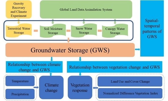
2. Methodology

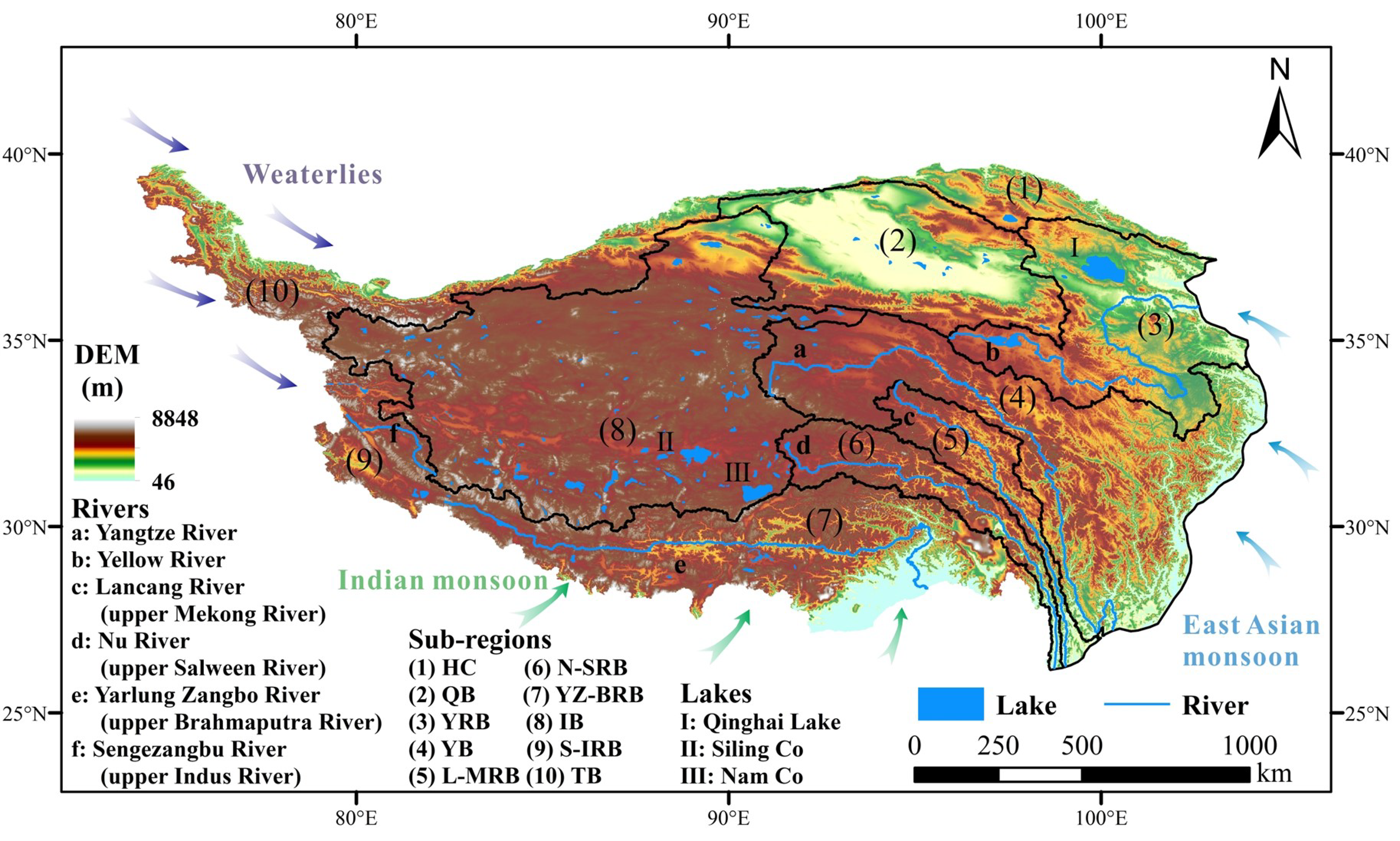
2.1. Study Area

The study area was in the geographic domain of the Tibetan Plateau (TP) in China and was composed of ten sub-regions with diverse geographical environments (Figure 1), including the Hexi Corridor (HC), the Qaidam Basin (QB), the Yellow River Basin (YRB), the Yangtze River Basin (YB), the Lancang River (upper Mekong River) Basin (L-MRB), the Nu River (upper Salween River) Basin (N-SRB), the Yarlung Zangbo River (upper Brahmaputra River) Basin (YZ-BRB), the Inner Basin (IB), the Sengezangbu River (upper Indus River) Basin (S-IRB), and the Tarim Basin (TB) [38].

These different sub-regions are characterized by different climate and hydrogeological conditions [3,39]. The western, eastern, and southern TP are affected by the westerlies, the East Asian monsoon, and the Indian monsoon, respectively, and other areas are generally controlled by a combination of two or three of these conditions. Therefore, the water cycle patterns in the TP will be significantly affected by large-scale atmospheric circulation [3]. The abundant precipitation caused by monsoons can greatly replenish large rivers on the edge of the TP. During 1980−2018, the annual runoff of these rivers showed different change characteristics, such as a significant increase in the Sengezangbu River (+3.9 Gt per decade), but a stable status in the Yangtze River and Nu River, while the Yellow River recorded a decline (–1.5 Gt per decade) during the same period [3]. In the center of the TP, there are numerous endorheic lakes, rather than large exorheic rivers, because of the lower annual precipitation level [39].

2.2. Data Sources

2.2.1. GRACE/FO

The CSR GRACE/FO RL06 mascon dataset has been frequently used in the study of terrestrial water storage changes due to its highest spatial resolution at this stage compared with other products [40,41,42]. The spatial resolution was 0.25 degrees. We used the GRACE data for 237 consecutive months (from April 2002 to December 2021). The cubic spline interpolation method was used to interpolate the short-term missing data of GRACE in the time series. For the long-term data interruption caused by the replacement of the GRACE and GRACE-FO satellites, the reconstruction method based on precipitation, which was invented in previous research, was used, and more detailed information regarding this method can be found in previous studies [43,44]. Additionally, all the grids used in this study were relative to the 2004–2009 mean baseline. The TWS was recorded in terms of equivalent water height (EWH) in cm.

2.2.2. GLDAS

The Global Land Data Assimilation System (GLDAS) uses data assimilation technology to fuse satellite-based data and in situ ground observation data to generate surface state quantities and fluxes that are closest to the observation data [45,46]. GLDAS includes four land surface models, NOAH, VIC, CLM, and MOSAIC. Compared with the other models, the NOAH model has the advantages of being an advanced model, having a high spatial resolution, and having a stable driving field. Thus, the model selected in this study was the GLDAS Noah Land Surface Model L4 monthly 0.25 × 0.25-degree V2.1 [47,48]. It has been widely used worldwide and is a highly recognized data source [24,45,46,49]. The spatial resolution is 0.25 degrees and is consistent with GRACE.

2.2.3. Temperature and Precipitation

Temperature (Tmp) and precipitation (Pre) are the most widely studied and important meteorological factors. Previous studies also showed that Tmp and Pre have significant effects on the variation in GWS [23,50].

The Climatic Research Unit gridded Time Series (CRU TS) can provide 0.5-degree-resolution monthly data covering the global land surface [51]. The dataset of Tmp and Pre from the CRU TS from April 2002 to December 2021 was used in this study. It is worth noting that the spatial resolution was interpolated to 0.25 degrees using the bilinear interpolation method to match the resolution of GRACE.

2.3. Vegetation Response

The vegetation response to the GWS changes was represented by the Normalized Difference Vegetation Index (NDVI) and Land Use and Cover Change (LUCC). The satellite-based NDVI, which has become the most popular index to reflect the state of regional climates and environments, is obtained by monitoring the vegetation growth status and estimating the vegetation coverage without damaging or altering the vegetation [52,53]. The satellite-based LUCC is one of the essential driving factors for regional climate variability, and its impact on hydrological cycle has become an important aspect of water resources [54,55]. The monthly data of the NDVI from April 2002 to December 2019 and the LUCC data of five periods in 2000, 2005, 2010, 2015, and 2020, were used in this study. The NDVI dataset is generated by calculating the maximum values of the first, middle, and last three ten days of each month. The LUCC types are divided into six first-level groups, which include cropland, forest, grassland, water, urban land, and unused land.

2.4. Method

2.4.1. Groundwater Storage Anomalies (GWSA)

The Terrestrial Water Storage Anomaly (TWSA) consists of four parts, namely, groundwater storage anomalies (GWSA), soil storage anomalies (SMSA), snow water equivalent anomalies (SWEA), and canopy water storage anomalies (CWSA) [26]. The GWSA could be isolated using the following formula [26]:

GWSA = TWSA − (SMSA + SWEA + CWSA)

(1)

where TWSAs were derived from gravity anomalies observed by GRACE/FO and the other three components were provided by GLDAS.

It should be emphasized that all data are also relative to the 2004–2009 mean baseline, meaning the value of the GWSA can be positive, negative, or zero. If the GWSA calculated for a certain pixel in a certain month are positive, this indicates that the GWSA in this area increase compared with the 2004–2009 mean baseline; a negative value indicates a decrease, and zero indicates no change.

2.4.2. Trend Test and Significance Analysis

Temporally, unitary linear regression analysis was used to construct a linear regression equation, and the k was used to quantify the trends as follows [52,56]:

$$k=\frac{n\times {\displaystyle \sum _{i=1}^n(i\times x_i)-{\displaystyle \sum _{i=1}^{n}i}\times {\displaystyle \sum _{i=1}^n{x}_i}}}{n\times {\displaystyle \sum _{i=1}^n{i}^2}-({\displaystyle \sum _{i=1}^{n}i}{)}^2}$$

(2)

where n is the number of months and x_i is variable in month i. If k > 0, the variables show a positive trend; otherwise, they would show a negative trend. k = 0 means no change.

Spatially, the change trend for various factors in each pixel was analyzed using the modified Mann–Kendall (MMK) test and represented by Slope [52,56,57,58,59]. Additionally, whether this trend has statistical significance was determined by t-tests. The corresponding formulas were as follows:

$$Slope=\mathrm{median}\left(\frac{x_j-x_k}{j-k}\right)\begin{array}{cc}& \end{array}(1\le k<j\le n)$$

(3)

$$\mathrm{sgn}(x_j-x_k)=\{\begin{array}{ll}1& x_j>x_k\\ 0& x_j=x_k\\ -1& x_j<x_k\end{array}$$

(4)

$$S={\displaystyle \sum _{k=1}^{n-1}{\displaystyle \sum _{j=k+1}^n\mathrm{sgn}(x_j-x_k)}}$$

(5)

$$Var(S)=\frac{n(n-1\left)\right(2n+5)}{18}$$

(6)

$$\eta =1+\frac{2}{n(n-1\left)\right(n-2)}\times {\displaystyle \sum _{k=1}^{n-1}(n-k)(n-k-1)(n-k)}{\rho }_{ACF}(k)$$

(7)

$$Z=\{\begin{array}{ll}\frac{S-1}{\sqrt{\eta \times Var(S)}}& \mathrm{for} S>0\\ \hfill 0\hfill & \mathrm{for} S=0\hfill \\ \frac{S+1}{\sqrt{\eta \times Var(S)}}& \mathrm{for} S<0\end{array}$$

(8)

Here, x_j is the parameter value at time j, and x_k at time k. Slope > 0 represents an upward trend; Slope < 0 represents a downward trend; and Slope = 0 means no change. ${\rho }_{ACF}(k)$ is the autocorrelation function (ACF) of the ranks of the observations [58]. The Z value indicates the trend of factors. In this study, the given significance levels were 99%, 95%, and 90%, when p = 0.01, 0.05, and 0.1, and |Z| − p/2 was equal to 2.58, 1.96, and 1.64, respectively [52,56]. Based on the factors trend, the nine levels were further divided and are presented in

Table 1. Index classification.

Level	Description of the Trend or Correlation	Slope or CC	p	|Z|
1	Extremely significant increase or positive correlation	>0	p < 0.01	|Z| > 2.58
2	Significant increase or positive correlation		0.01 < p ≤ 0.05	1.96 < |Z| ≤ 2.58
3	Weakly significant increase or positive correlation		0.05 < p ≤ 0.1	1.64 < |Z| ≤ 1.96
4	Insignificant increase or positive correlation		p > 0.1	|Z| ≤ 1.64
5	Extremely significant decrease or negative correlation	<0	p < 0.01	|Z| > 2.58
6	Significant decrease or negative correlation		0.01 < p ≤ 0.05	1.96 < |Z| ≤ 2.58
7	Weakly significant decrease or negative correlation		0.05 < p ≤ 0.1	1.64 < |Z| ≤ 1.96
8	Insignificant decrease or negative correlation		p > 0.1	|Z| ≤ 1.64
9	Unchanged or uncorrelated	=0	-	-

.

2.4.3. Correlation Analysis

The correlation analysis method was used to analyze the relationship between two variables in each pixel [52]. The corresponding formula was as follows:

$$C{C}_{xy}=\frac{{\displaystyle \sum _{i=1}^n\left[(x_i-\overline{x})(y_i-\overline{y})\right]}}{\sqrt{{\displaystyle \sum _{i=1}^n{(x_i-\overline{x})}^2}{\displaystyle \sum _{i=1}^n{(y_i-\overline{y})}^2}}}$$

(9)

where CC_xy represents the correlation coefficient (CC) between variables x and y; x_i and y_i represent the value of the variables x and y in month I, respectively; and $\overline{x}$ and $\overline{y}$ are the mean value of the variables x and y, respectively. The CC ranged from −1 to 1. There was a positive correlation when the CC was greater than 0 and a negative correlation when it was less than 0. Additionally, the significance of the results was evaluated using a t-test, and it could be divided into four groups, extremely significant, significant, weakly significant, and insignificant. Thus, the relationships between the dependent variable and independent variable were further divided into nine levels, as detailed in Table 1.

3. Results and Discussion

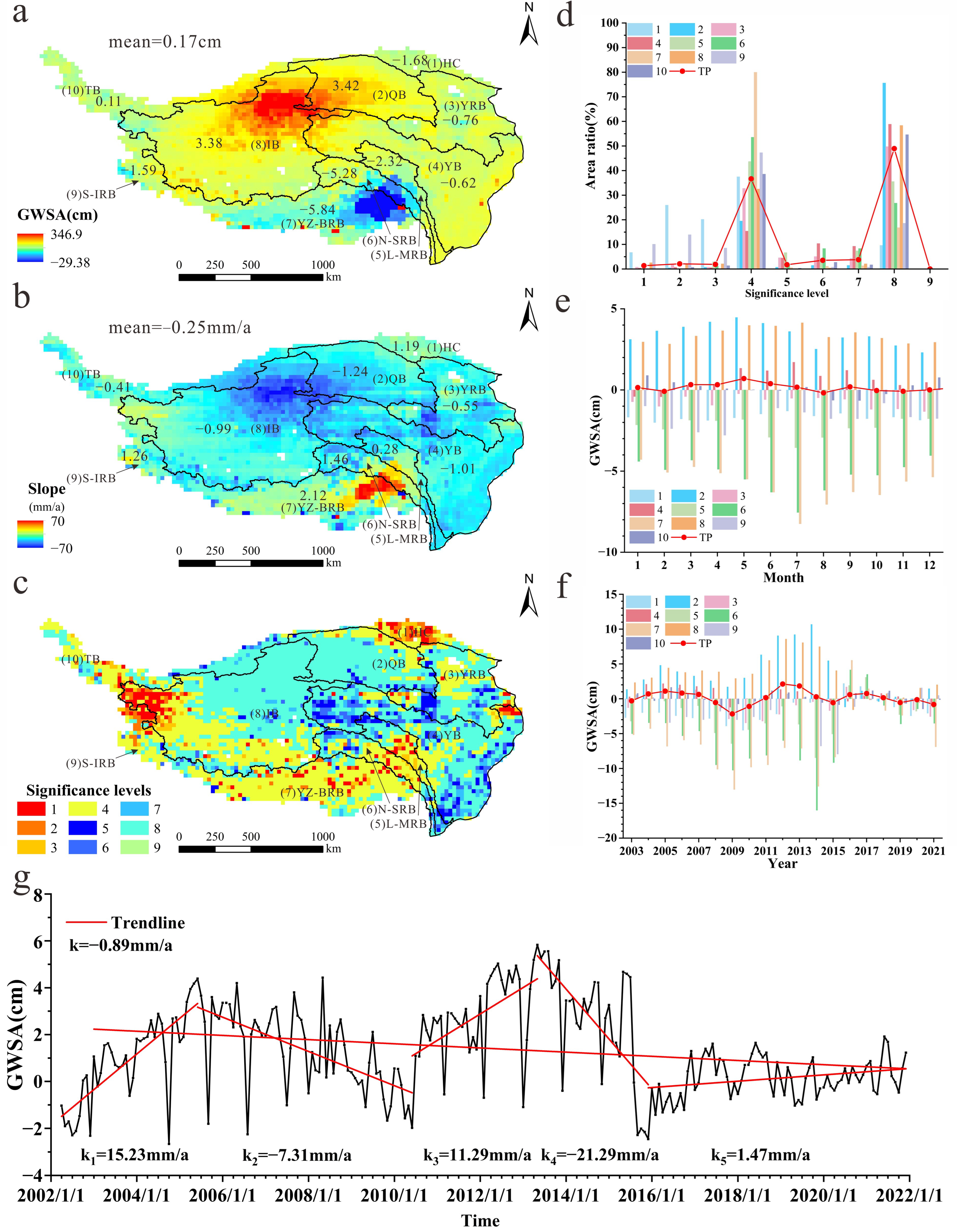
3.1. Spatial–Temporal Patterns of GWSA

The GWSA across the TP had obvious spatial heterogeneity, with a mean of 0.17 cm (Figure 2a) and a decreasing rate of −0.25 mm/a (Figure 2b). The higher values were mainly distributed in the QB, the IB, the source of the Yangtze River, and the southeastern edge of the TP. The difference in the GWSA reached 9.26 mm. The value of the GWSA in the QB was the highest, 3.42 cm, ranking first in the sub-regions. However, it had been decreasing with the highest decreasing rate of −1.24 mm/a (Figure 2b) and in a large area of 79.3% of the region (Figure 2c). On the contrary, the YZ-BRB had the lowest GWSA of −5.84 cm, with the highest increasing rate at 2.12 mm/a and a large increasing area of 80.2% of the basin. Furthermore, it revealed an increasing trend in 42.0% of the plateau area, while a decreasing trend was present in 58.0% of the plateau area (Figure 2c,d). The areas where the slope of the GWSA was positive were mainly HC, S-IRB, YZ-BRB, and south and southwest of the IB. In the HC and S-IRB, 53.9% and 33.3% of the regions showed a significant increasing trend, and a significant decrease was observed in <2% of these two basins, which indicated that the GWS levels in these sub-regions were increasing. In the YB and the YRB, 83.0% and 63.7% showed a decreasing trend, while 31.2% and 17.0% showed a significant decreasing trend, respectively.

The GWSA varied seasonally, with an increase in rainy seasons (May–October) and a decrease in dry seasons (November to April in the next year) (Figure 2e). The difference in the GWSA in the YB reached 1.06 cm, where the GWSA in rainy seasons and dry seasons were 1.15 cm and 0.09 cm, respectively. The variation in the GWSA in the YB was consistent with the variation in rainfall, indicating that the annual variation in groundwater may be affected by the recharge of rainfall. The GWSA of the IB in rainy seasons and dry seasons were 3.67 cm and 3.09 cm, respectively. As the amount of precipitation in this basin is still less in the rainy season, it is possible that permafrost degradation and glacier melting caused by increasing temperature have a stronger impact on the GWS than precipitation. The minimum negative anomaly of the interannual variation in the GWSA was −2.16 cm in 2009, while the maximum positive anomaly of 2.11 cm occurred in 2012 (Figure 2f). Although the GWS increased rapidly from 2009 to 2012, it was still declining overall from 2003 to 2021, which was similar to the result inferred from the monthly GWSA from April 2002 to December 2021 (Figure 2g). The latter was divided into five periods, April 2002 to June 2005, July 2005 to June 2010, June 2010 to May 2013, June 2013 to December 2015, and January 2016 to December 2021. Overall, the GWS in the TP was decreasing at an average rate of −0.89 mm/a from January 2003 to December 2021. Despite the lowest GWSA value of −2.66 cm occurring in October 2004, the GWS was still rising at a speed of 15.23 mm/a from April 2002 to June 2005. Then, there was a 60-month decrease at −7.31 mm/a from July 2005 to June 2010. The third period, from June 2010 to May 2013, was an increasing period. The increasing speed was 11.29 mm/a, and the GWSA reached the maximum value of 5.82 cm in May 2013. The largest decrease rate of −21.29 mm/a occurred from June 2013 to December 2015. It had been slowly rising since January 2016, with a speed of 1.47 mm/a. The results of the study by Liu et al. [22] were the same. Liu et al. [22] also came to a similar conclusion that GWS in the Qinghai province and the Tibet Autonomous Region reached a split point in 2016, and the groundwater storage changed from decreasing with a mean rate of −0.2 mm/a from 2003 to 2015 to increasing with a mean rate of 3.28 mm/a from 2016 to 2019. The GWSA in the TP showed an overall downward trend, but increases after 2016. This shows that the amount of groundwater storage is gradually recovering.

3.2. The Influence of Climate Change on GWS in the TP

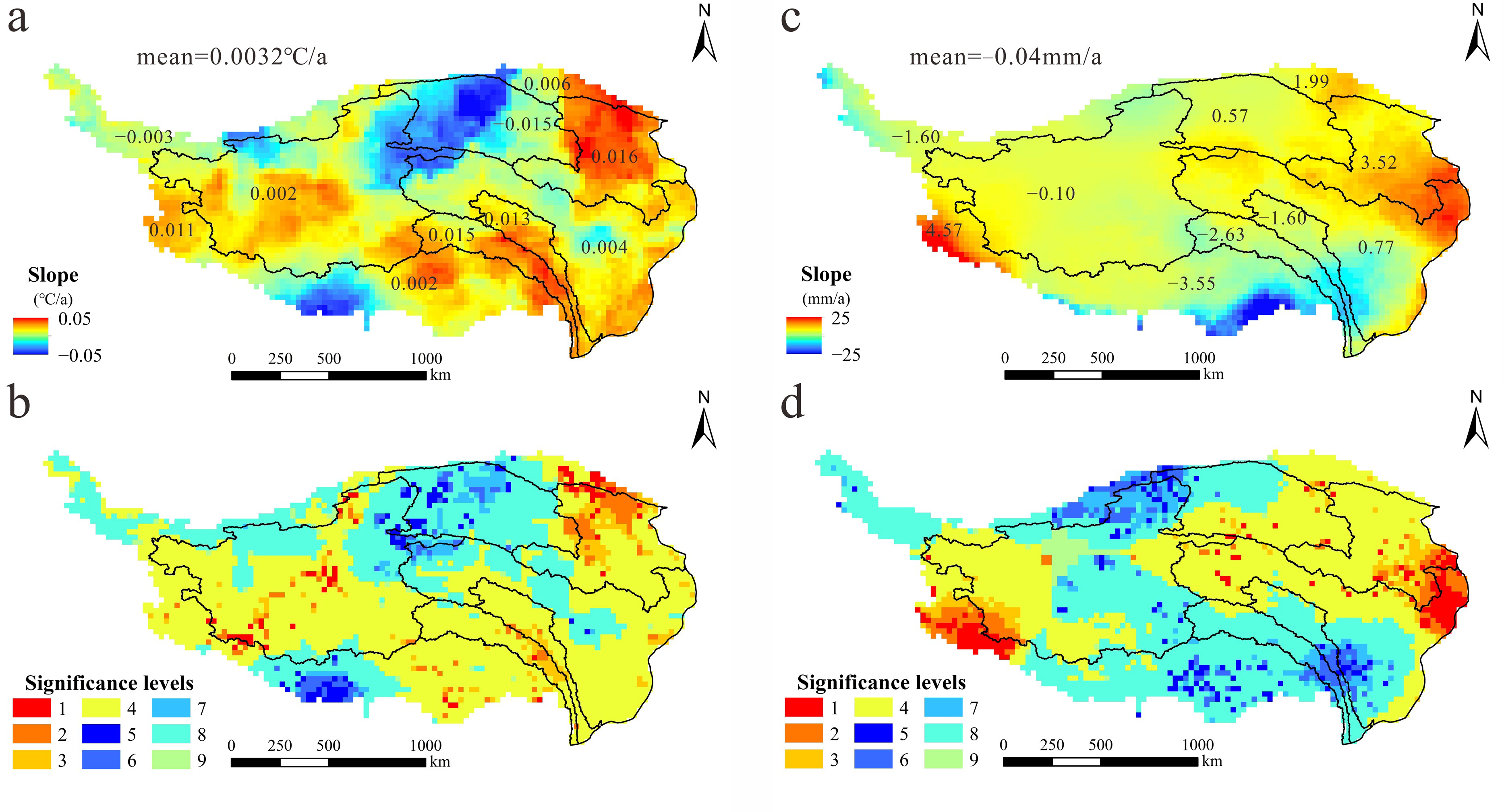
3.2.1. Fluctuation Characteristics of Regional Climate

The changes in temperature and precipitation were calculated, and the spatial characteristics of climate change are shown in Figure 3.

As shown in Figure 3a,b, the changes indicate that the temperature increased in 64.1% of the TP and decreased in 35.1% of the TP. The areas where the temperature increased were mainly distributed in the YRB, the L-MRB, the N-SRB, the S-IRB, the east of the YB, the east of the YZ-BRB, and the south of the IB. The increase rate of the temperature in the YRB was 0.016 °C/a. Additionally, 89.0% of the YRB showed an increasing trend. The decrease rate of the temperature in the QB, in which 88.3% showed a decreasing trend, was −0.015 °C/a.

The precipitation showed a decreasing trend at −0.04 mm/a and in 49.6% of the TP from 2003 to 2021, mainly over the YZ-BRB, the N-SRB, the TB, the south of the YB, the south of the L-MRB, the center of the IB, and the northwest of the QB (Figure 3c,d). The Brahmaputra River Basin had the highest decreasing rate of −3.55 mm/a and a decreasing area of 90.5%. Meanwhile, the largest increase in precipitation was shown to be in the Indus River Basin, with an increasing rate of 4.57 mm/a and an increasing area of 92.4%. These results indicate that there have been different or even opposite trends in the rate of climate change in different sub-regions of the TP in recent years.

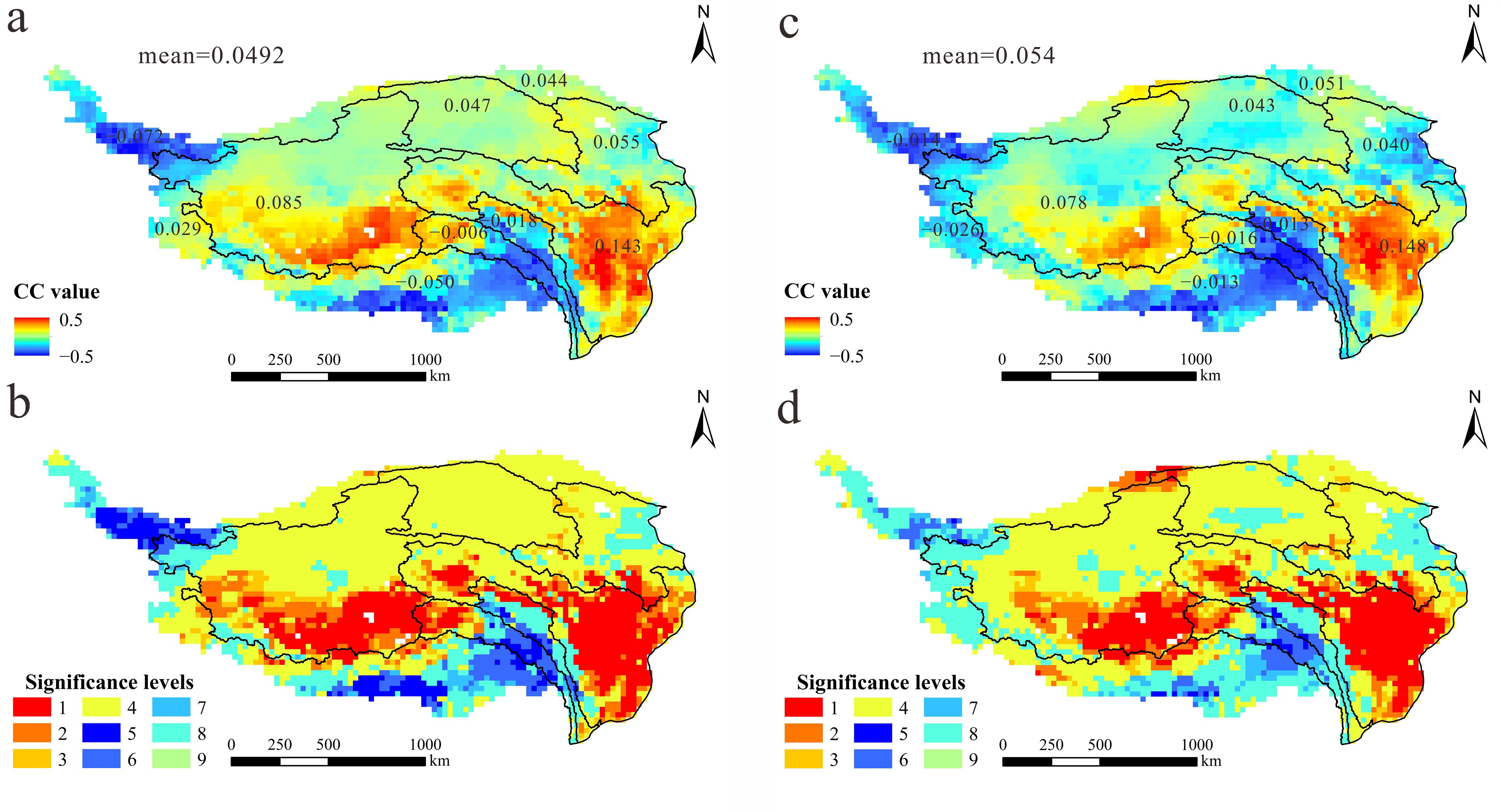
3.2.2. Relationship between Climate Change and GWS

The correlation coefficients between the GWSA and Tmp and Pre were calculated to analyze the relationships between the GWS and climate change. Then, significance tests were carried out. The results are shown in Figure 4.

Overall, the GWSA were positively correlated with Tmp, and the mean correlation coefficient was 0.0492 (Figure 4a). The correlation coefficient in the YB was 0.143, which was the highest among the ten sub-regions. The HC, the QB, the YRB, the YB, the IB, and the S-IRB were the main regions that showed positive correlations. This shows that the areas that had positive correlations accounted for about 74.94% of the study area. In these areas, 15.23% showed extremely significant positive correlations. There were mostly insignificant positive correlations in 47.51% of the study area, which were mainly the HC, the QB, and the YRB (Figure 4b). The negatively correlated area covered 25.06% of the study area, with insignificant negative correlation occupying 13.66% of the area (Figure 4a,b). In the L-MRB, the N-SRB, the YZ-BRB, and the TB, the GWSA were insignificantly negatively correlated with the temperature in 25.87% of the area.

As shown in Figure 4c, the mean correlation coefficient was 0.054, which was greater than 0, indicating a positive correlation between the GWSA and Pre in the TP. The variables were positively correlated in 70.81% of the study area and negatively correlated in 29.19% of the study area. The mean correlation coefficient was 0.148 in the YB, which was the highest among the ten sub-regions. The L-MRB, the N-SRB, the YZ-BRB, the IB, and the TB were the main regions showing negative correlations, accounting for 68.24% of the negatively correlated areas in total. The results of the significance tests in Figure 4d indicate that the GWSA were extremely significantly positively correlated with precipitation in 13.96% of the TP, mainly in the YB and south of the IB.

Increasing precipitation will lead to more groundwater recharge, and thus, an increase in the GWS. Precipitation in the TP has been slightly increasing since the 1960s and is projected to further increase in the future in most areas of the TP [60]. The direct manifestation of permafrost degradation caused by increased temperature is the increase in the number and area of thermal karst lakes, which leads to the reduction in GWS in the form of runoff or evaporation [61,62]. However, when a large number of glaciers are distributed in the basin, the increase in glacial meltwater caused by the increase in temperature will recharge the groundwater, weaken the decrease in GWS, and even cause the increase in GWS. This is the reason why the GWS in the north and south of the IB showed different trends. There are many glaciers in the southern part of the IB and almost no glaciers in the northern part of the IB. Similar results were obtained in previous studies in the central Qiangtang Nature Reserve and the Upper Indus Basin [16]. The GWS in the L-MRB, N-SRB, and YZ-BRB increased in the context of decreased precipitation and increased temperature. As decreased precipitation and increased glacial melt due to temperature increases may cause decreased GWS, these three regions may require more groundwater recharge. The decreased GWS in the YRB and YB, where the temperature and precipitation increased, may indirectly support this hypothesis that the groundwater in the YRB and YB may seep to the L-MRB, N-SRB, and YZ-BRB [16].

3.3. Ecological Effect of Groundwater Storage

3.3.1. Vegetation Change

As shown in Figure 5, grassland has the largest area of 84.285 × 10⁴ km² of the TP (

Table 2. Area of different land use types in 2020 and changed area from 2000 to 2020 (10⁴ km²).

Basin		Cropland	Forest	Grassland	Water	Urban Land	Unused Land
HC	Area	0.009	0.382	2.181	0.200	0.002	2.027
	Changed area	0.002	0.001	0.017	0.080	0.001	−0.125
QB	Area	0.061	0.169	5.730	0.522	0.035	12.090
	Changed area	0.009	−0.006	0.106	0.171	0.015	−0.294
YRB	Area	0.634	2.022	12.367	0.696	0.093	2.121
	Changed area	−0.010	0.015	0.654	0.066	0.033	−0.762
YB	Area	0.745	9.313	18.935	0.723	0.041	3.197
	Changed area	0.044	0.388	0.210	0.059	0.023	−0.694
L-MRB	Area	0.150	1.720	3.870	0.063	0.003	0.398
	Changed area	0.046	0.242	−0.060	0.028	0.002	−0.247
N-SRB	Area	0.046	1.664	4.429	0.166	0.005	1.266
	Changed area	−0.001	0.355	0.128	−0.032	0.004	−0.447
YZ-BRB	Area	0.339	7.097	11.342	1.093	0.027	5.920
	Changed area	0.090	0.920	−2.278	−0.158	0.019	1.486
IB	Area	0.001	0.692	21.507	4.752	0.002	22.990
	Changed area	0.001	0.681	−14.926	2.022	0.002	12.284
S-IRB	Area	0.001	0.376	3.036	0.375	0.002	2.962
	Changed area	0.001	0.374	−1.840	0.164	0.002	1.321
TB	Area	0.007	0.023	5.889	0.989	0.001	6.765
	Changed area	0.006	−0.001	0.800	−0.449	0.001	−0.342
The TP	Area	1.994	23.457	89.285	9.577	0.210	59.736
	Changed area	0.19	2.97	−17.19	1.96	0.10	12.18

), mostly distributed in the IB, YB, YRB, and YZ-BRB. The area of unused land has the second largest area, which is 59.736 × 10⁴ km², mainly covering the IB and QB. The forest land that is mainly distributed in the YB and YZ-BRB covers 23.457 × 10⁴ km². The area of water, mainly lakes and glaciers, is 9.577 × 10⁴ km². The cropland and urban land types cover 1.994 × 10⁴ km² and 0.210 × 10⁴ km², respectively, which means there is a low level of human activity on the TP. However, these areas have increased by 0.19 × 10⁴ km² and 0.10 × 10⁴ km² from 2000 to 2020, respectively, indicating that human activities cannot be ignored.

The highest decrease and increase in land cover changes from 2000 to 2020 were grassland and unused land, with changed areas of −17.19 × 10⁴ km² and 12.18 × 10⁴ km², respectively. This means that large areas of grassland have degraded to sand, desert, and other kinds of unused land, especially in the IB, where the area of grassland decreased to 14.926 × 10⁴ km² and the unused land increased to 12.284 × 10⁴ km². It should be noted that different trends occurred in the LUCC of the YRB and YB. The area of unused land decreased while the area of forest and grassland increased, which proved the effectiveness of ecological protection and construction projects, such as eco-migration, grazing bans, forest and wetland reservations, etc. [16,63].

As LUCC is discrete data, it is difficult to quantify the vegetation response to GWS. Therefore, the influences of groundwater change on vegetation in time and space were discussed using the NDVI, an indicator of vegetation change.

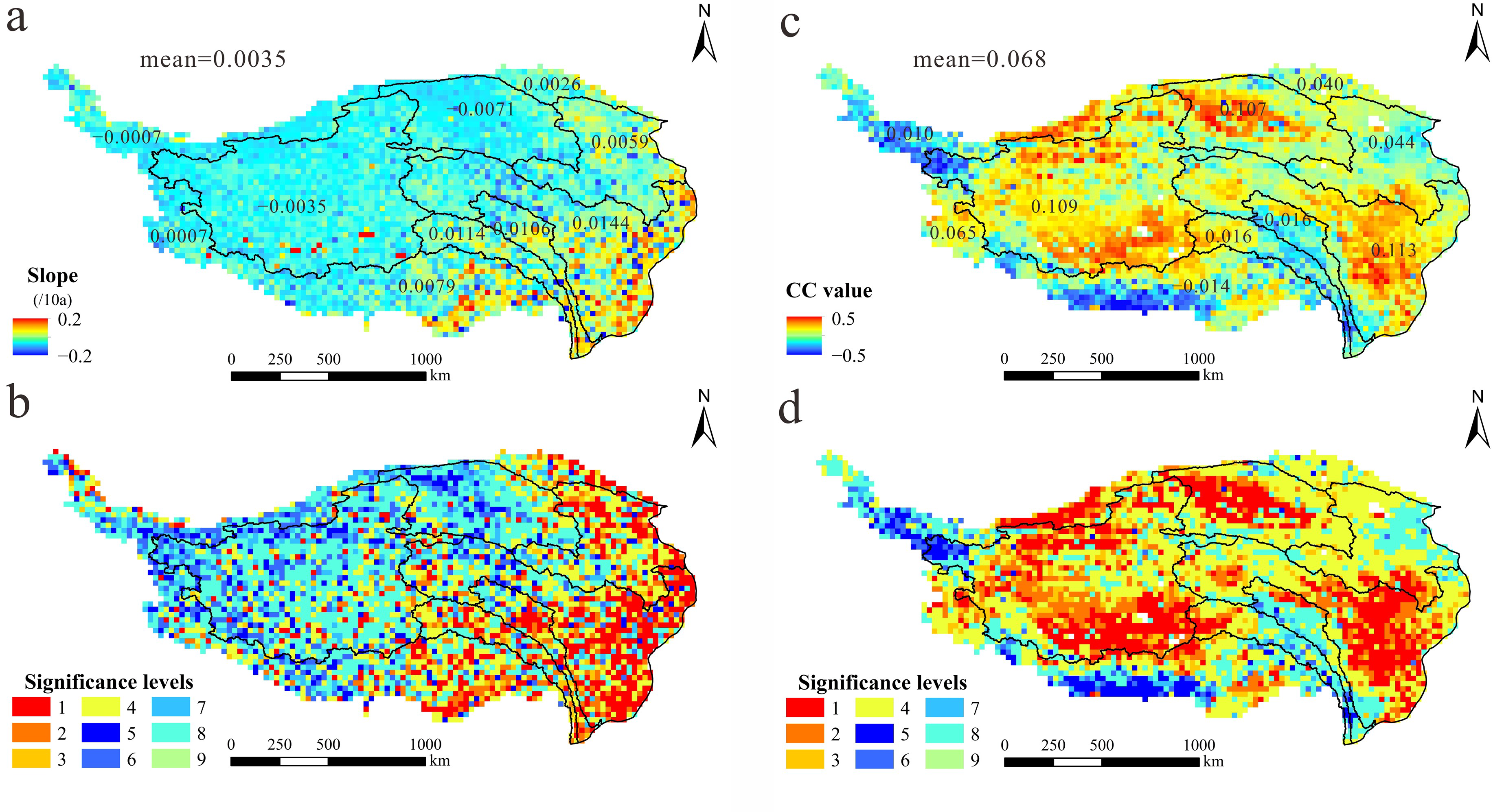
3.3.2. Vegetation Responses to GWS Changes

Overall, the NDVI increased with the mean rate of 0.0035 per ten years, but the increase was lower in the west and faster in the east from 2003 to 2019 (Figure 6a). The YB showed the fastest increasing rate of 0.0144 per ten years, while the lowest was in the QB, with a rate of −0.0071 of per ten years. The areas where the NDVI increased significantly are mainly distributed over the east edge of the TP (Figure 6b). In Figure 6c, it can be seen that the GWS and the NDVI were positively correlated, and the correlation coefficient was 0.068. Additionally, they had a positive correlation relationship in 73.17% of the study area. The highest correlation coefficient was 0.113 in the YB, while the lowest was −0.016 in the L-MRB. The weakly to extremely significant positive correlations were in 36.91% of the aforementioned areas, mostly in the QB, YB, and YZ-BRB (Figure 6d). The regions where there was a negative correlation between the GWS and the NDVI covered 26.83% of the TP, of which only 23.59% were significantly or extremely significantly negatively correlated (Figure 6d).

The GWS was positively correlated with the NDVI, which indicated that the vegetation was dependent on the groundwater condition. In the IB, large areas of grassland have degenerated into unused land because of the decline in the groundwater level in the context of climate change [64,65]. This is analogous to the earlier findings reported in the TP. Peng et al. [66] also found that the decline of the groundwater level in the source area of the Yellow River was closely related to the deterioration of the ecological environment in the permafrost-degraded area. This may have been due to the decrease in the groundwater level, which would have caused a great loss to occur in the shallow soil moisture, which would have meant that the root system of some vegetation in cold areas could not effectively use soil water, eventually leading to the degradation or disappearance of vegetation [67,68,69].

4. Conclusions

Based on the linear regression and modified Mann–Kendall test analysis methods, the temporal and spatial variations in GWS were analyzed using the GRACE and GLDAS data from April 2002 to December 2021. Then, the driving factors and ecological effects of the changes in GWS in the Tibetan Plateau were discussed, using the correlation analysis model and multi-source remote sensing data. This study of groundwater storage changes provides a useful reference for ecological protection and the high-quality development of the TP. The conclusions are as follows:

• The higher values were mainly distributed in the QB, the IB, the source of the Yangtze River, and the southeastern edge of the TP. An increasing trend in the GWS was revealed in 42.0% of the plateau area and a decreasing trend was revealed in 58.0% of the plateau area. The areas where the GWS increased were mainly the HC, S-IRB, YZ-BRB, and the south and southwest of the IB.
• Overall, the GWS in the TP was decreasing at an average rate of −0.89 mm/a from January 2003 to December 2021. However, the GWS has been slowly rising at a rate of 1.47 mm/a since January 2016. This shows that the level of groundwater storage is gradually recovering.
• The different climate conditions in the different sub-regions had different impacts on the change in the GWS. The change in precipitation may be the main reason for the change in the GWS in the YB. Rising temperatures have a two-sided effect on the groundwater storage. On the one hand, the melting of ice and snow caused by rising temperatures will replenish the groundwater, which will increase the groundwater storage in some areas, such as the south of the IB. On the other hand, permafrost degradation caused by climate change will lead to a decrease in the GWS in other regions, such as the north of the IB.
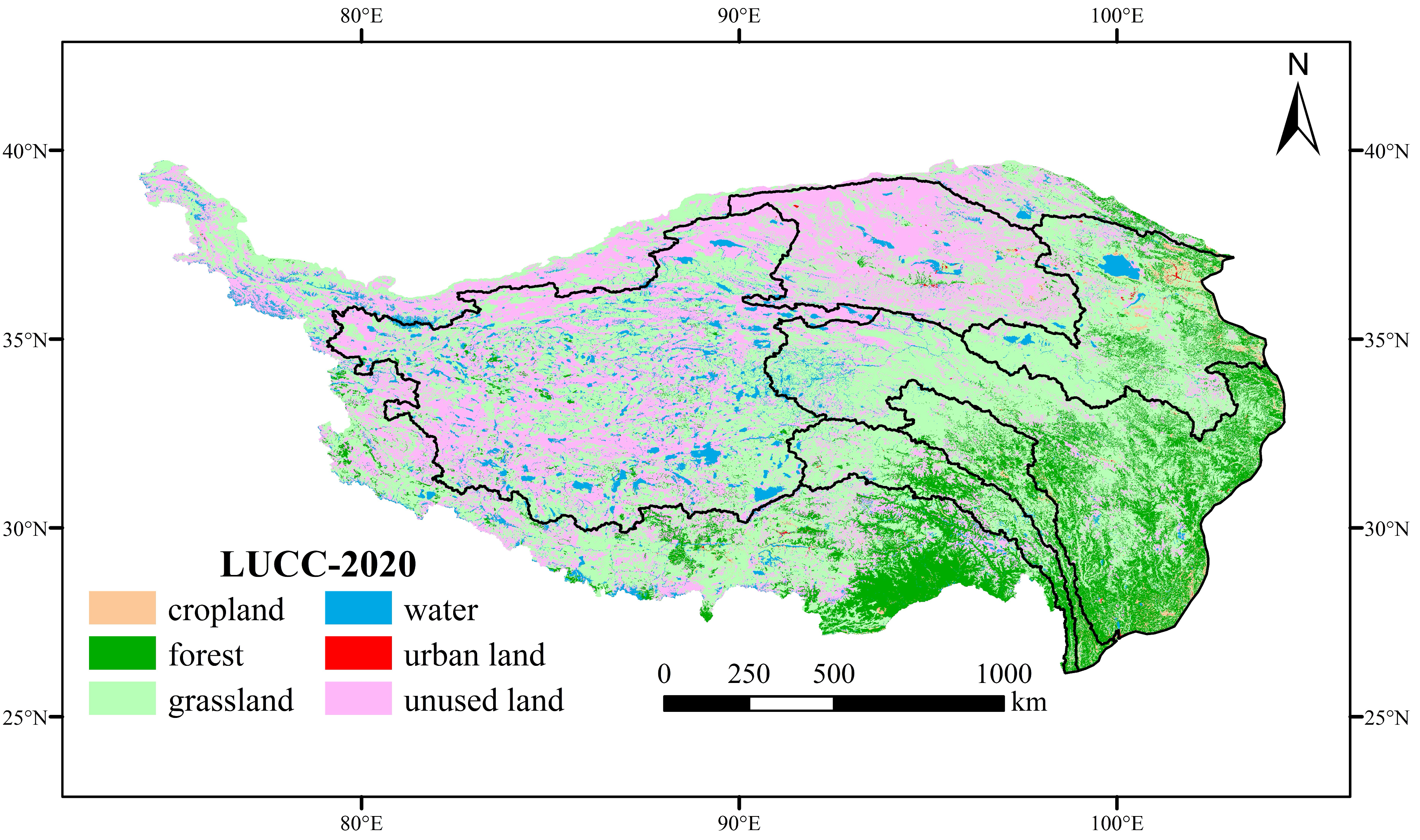
• The potential ecological effects were investigated, with the results showing that the reduction in the GWS is an important cause of vegetation degradation. The decrease in the GWS reduced the efficiency of plant roots in absorbing and utilizing groundwater and eventually led to the degradation of 17.19 × 10⁴ km² of grassland to sand, desert, or other kinds of unused land on the TP.

The results of this study could offer a new opportunity to reveal the groundwater changes in a cryosphere region and to assess the impact of the changes in hydrological conditions on ecology. However, this study only provided a preliminary investigation of the changes to GWS, and more in-depth studies should focus on the following specific aspects: (1) in situ groundwater monitoring with high temporal and spatial resolution at the regional scale to gain insight into the accurate variation mechanism of groundwater storage on the TP; (2) the integration of multivariate satellite data and improving modeling capacity to deal with the quality change signals caused by rapid structural uplift; (3) the quantitative analysis of the response of groundwater to climate change and the evaluation of the effects of groundwater changes on vegetation evolution under climate change.

References

- Yao, T.; Masson-Delmotte, V.; Gao, J.; Yu, W.; Yang, X.; Risi, C.; Sturm, C.; Werner, M.; Zhao, H.; He, Y.; et al. A review of climatic controls on δ18O in precipitation over the Tibetan Plateau: Observations and simulations. Rev. Geophys. 2013, 51, 525–548. [Google Scholar] [CrossRef]
- Wang, J.; Huang, L.; Ju, J.; Daut, G.; Ma, Q.; Zhu, L.; Haberzettl, T.; Baade, J.; Mäusbacher, R.; Hamilton, A.; et al. Seasonal stratification of a deep, high-altitude, dimictic lake: Nam Co, Tibetan Plateau. J. Hydrol. 2020, 584, 124668. [Google Scholar] [CrossRef]
- Yao, T.; Bolch, T.; Chen, D.; Gao, J.; Immerzeel, W.; Piao, S.; Su, F.; Thompson, L.; Wada, Y.; Wang, L.; et al. The imbalance of the Asian water tower. Nat. Rev. Earth Environ. 2022, 3, 618–632. [Google Scholar] [CrossRef]
- Chen, D.; Tan-Dong, Y. Climate change and its impact on the Third Pole and beyond. Adv. Clim. Chang. Res. 2021, 12, 297–298. [Google Scholar] [CrossRef]
- Xiaodong, L.; Baode, C. Climatic warming in the Tibetan Plateau during recent decades. Int. J. Climatol. 2000, 20, 1729–1742. [Google Scholar] [CrossRef]
- Kang, S.; Xu, Y.; You, Q.; Fluegel, W.-A.; Pepin, N.; Yao, T. Review of climate and cryospheric change in the Tibetan Plateau. Environ. Res. Lett. 2010, 5, 015101. [Google Scholar] [CrossRef]
- Li, X.; Long, D.; Scanlon, B.R.; Mann, M.E.; Li, X.; Tian, F.; Sun, Z.; Wang, G. Climate change threatens terrestrial water storage over the Tibetan Plateau. Nat. Clim. Chang. 2022, 12, 801–807. [Google Scholar] [CrossRef]
- Yao, T.D.; Thompson, L.; Yang, W.; Yu, W.S.; Gao, Y.; Guo, X.J.; Yang, X.X.; Duan, K.Q.; Zhao, H.B.; Xu, B.Q.; et al. Different glacier status with atmospheric circulations in Tibetan Plateau and surroundings. Nat. Clim. Chang. 2012, 2, 663–667. [Google Scholar] [CrossRef]
- He, Z.; Yang, W.; Wang, Y.J.; Zhao, C.X.; Ren, S.T.; Li, C.H. Dynamic Changes of a Thick Debris-Covered Glacier in the Southeastern Tibetan Plateau. Remote Sens. 2023, 15, 357. [Google Scholar] [CrossRef]
- Yongsheng, Z.; Li, T.; Bin, W. Decadal change of the spring snow depth over the Tibetan Plateau: The associated circulation and influence on the East Asian summer monsoon. J. Clim. 2004, 17, 2780–2793. [Google Scholar] [CrossRef]
- Zhaoxia, P.; Xu, L.; Salomonson, V.V. MODIS/Terra observed seasonal variations of snow cover over the Tibetan Plateau. Geophys. Res. Lett. 2007, 34, 137–161. [Google Scholar] [CrossRef]
- Zhang, G.Q.; Xie, H.J.; Kang, S.C.; Yi, D.H.; Ackley, S.F. Monitoring lake level changes on the Tibetan Plateau using ICESat altimetry data (2003-2009). Remote Sens. Environ. 2011, 115, 1733–1742. [Google Scholar] [CrossRef]
- Zhang, G.; Yao, T.; Xie, H.; Yang, K.; Zhu, L.; Shum, C.K.; Bolch, T.; Yi, S.; Allen, S.; Jiang, L.; et al. Response of Tibetan Plateau lakes to climate change: Trends, patterns, and mechanisms. Earth-Sci. Rev. 2020, 208, 103269. [Google Scholar] [CrossRef]
- Ren, W.; Tian, L.D.; Shao, L.L. Temperature and precipitation control the seasonal patterns of discharge and water isotopic signals of the Nyang River on the southeastern Tibetan Plateau. J. Hydrol. 2023, 617, 129064. [Google Scholar] [CrossRef]
- Immerzeel, W.W.; Droogers, P.; de Jong, S.M.; Bierkens, M.F.P. Large-scale monitoring of snow cover and runoff simulation in Himalayan river basins using remote sensing. Remote Sens. Environ. 2009, 113, 40–49. [Google Scholar] [CrossRef]
- Xiang, L.; Wang, H.; Steffen, H.; Wu, P.; Jia, L.; Jiang, L.; Shen, Q. Groundwater storage changes in the Tibetan Plateau and adjacent areas revealed from GRACE satellite gravity data. Earth Planet. Sci. Lett. 2016, 452, 309. [Google Scholar] [CrossRef]
- Deng, H.J.; Pepin, N.C.; Liu, Q.; Chen, Y.N. Understanding the spatial differences in terrestrial water storage variations in the Tibetan Plateau from 2002 to 2016. Clim. Chang. 2018, 151, 379–393. [Google Scholar] [CrossRef]
- Gao, G.; Zhao, J.; Wang, J.; Zhao, G.; Chen, J.; Li, Z. Spatiotemporal Variation and Driving Analysis of Groundwater in the Tibetan Plateau Based on GRACE Downscaling Data. Water 2022, 14, 3302. [Google Scholar] [CrossRef]
- Khorrami, B.; Gunduz, O. Evaluation of the temporal variations of groundwater storage and its interactions with climatic variables using GRACE data and hydrological models: A study from Turkey. Hydrol. Process. 2021, 35, 3406–3425. [Google Scholar] [CrossRef]
- Han, Z.; Huang, S.; Huang, Q.; Bai, Q.; Leng, G.; Wang, H.; Zhao, J.; Wei, X.; Zheng, X. Effects of vegetation restoration on groundwater drought in the Loess Plateau, China. J. Hydrol. 2020, 591, 125566. [Google Scholar] [CrossRef]
- Zhang, H.; Ding, J.; Wang, Y.; Zhou, D.; Zhu, Q. Investigation about the correlation and propagation among meteorological, agricultural and groundwater droughts over humid and arid/semi-arid basins in China. J. Hydrol. 2021, 603, 127007. [Google Scholar] [CrossRef]
- Liu, F.; Kang, P.; Zhu, H.; Han, J.; Huang, Y. Analysis of Spatiotemporal Groundwater-Storage Variations in China from GRACE. Water 2021, 13, 2378. [Google Scholar] [CrossRef]
- Ahmed, M.; Aqnouy, M.; El Messari, J.S. Sustainability of Morocco’s groundwater resources in response to natural and anthropogenic forces. J. Hydrol. 2021, 603, 126866. [Google Scholar] [CrossRef]
- Sliwinska, J.; Birylo, M.; Rzepecka, Z.; Nastula, J. Analysis of Groundwater and Total Water Storage Changes in Poland Using GRACE Observations, In-situ Data, and Various Assimilation and Climate Models. Remote Sens. 2019, 11, 2949. [Google Scholar] [CrossRef]
- Hu, W.; Liu, H.; Bao, A.; El-Tantawi, A.M. Influences of environmental changes on water storage variations in Central Asia. J. Geogr. Sci. 2018, 28, 985–1000. [Google Scholar] [CrossRef]
- Liu, X.; Hu, L.; Sun, K.; Yang, Z.; Sun, J.; Yin, W. Improved Understanding of Groundwater Storage Changes under the Influence of River Basin Governance in Northwestern China Using GRACE Data. Remote Sens. 2021, 13, 2672. [Google Scholar] [CrossRef]
- Yang, K.; Wu, H.; Qin, J.; Lin, C.; Tang, W.; Chen, Y. Recent climate changes over the Tibetan Plateau and their impacts on energy and water cycle: A review. Glob. Planet. Chang. 2014, 112, 79–91. [Google Scholar] [CrossRef]
- Luo, J.; Ke, C.-Q.; Seehaus, T. The West Kunlun Glacier Anomaly and Its Response to Climate Forcing during 2002–2020. Remote Sens. 2022, 14, 3465. [Google Scholar] [CrossRef]
- Xu, L.; Gao, B. Understanding the Effects of Cold and Warm Season Air Warming on the Permafrost Hydrology Changes in the Source Region of the Lancang River, the Qinghai-Tibetan Plateau. J. Geophys. Res.-Atmos. 2022, 127, e2022JD036551. [Google Scholar] [CrossRef]
- Li, F.W.; Wang, Y.; Zhao, Y.; Qiao, J.L. Modelling the response of vegetation restoration to changes in groundwater level, based on ecologically suitable groundwater depth. Hydrogeol. J. 2018, 26, 2189–2204. [Google Scholar] [CrossRef]
- Zhang, H.; Wang, X.-S. The impact of groundwater depth on the spatial variance of vegetation index in the Ordos Plateau, China: A semivariogram analysis. J. Hydrol. 2020, 588, 125096. [Google Scholar] [CrossRef]
- Xu, M.; Kang, S.; Chen, X.; Wu, H.; Wang, X.; Su, Z. Detection of hydrological variations and their impacts on vegetation from multiple satellite observations in the Three-River Source Region of the Tibetan Plateau. Sci. Total Environ. 2018, 639, 1220–1232. [Google Scholar] [CrossRef]
- Wei, Y.Y.; Sun, S.G.; Liang, D.; Jia, Z.H. Spatial-temporal variations of NDVI and its response to climate in China from 2001 to 2020. Int. J. Digit. Earth 2022, 15, 1463–1484. [Google Scholar] [CrossRef]
- Gao, Y.; Zhou, X.; Wang, Q.; Wang, C.; Zhan, Z.; Chen, L.; Yan, J.; Qu, R. Vegetation net primary productivity and its response to climate change during 2001–2008 in the Tibetan Plateau. Sci. Total Environ. 2013, 444, 356–362. [Google Scholar] [CrossRef] [PubMed]
- Piao, S.; Tan, K.; Nan, H.; Ciais, P.; Fang, J.; Wang, T.; Vuichard, N.; Zhu, B. Impacts of climate and CO2 changes on the vegetation growth and carbon balance of Qinghai–Tibetan grasslands over the past five decades. Glob. Planet. Chang. 2012, 98–99, 73–80. [Google Scholar] [CrossRef]
- Zhang, B.; Zhou, W. Spatial-Temporal Characteristics of Precipitation and Its Relationship with Land Use/Cover Change on the Qinghai-Tibet Plateau, China. Land 2021, 10, 269. [Google Scholar] [CrossRef]
- Xu, W.; Su, X. Challenges and impacts of climate change and human activities on groundwater-dependent ecosystems in arid areas–A case study of the Nalenggele alluvial fan in NW China. J. Hydrol. 2019, 573, 376–385. [Google Scholar] [CrossRef]
- Zhang, G.Q.; Yao, T.D.; Xie, H.J.; Kang, S.C.; Lei, Y.B. Increased mass over the Tibetan Plateau: From lakes or glaciers? Geophys. Res. Lett. 2013, 40, 2125–2130. [Google Scholar] [CrossRef]
- Li, Y.; Su, F.; Chen, D.; Tang, Q. Atmospheric Water Transport to the Endorheic Tibetan Plateau and Its Effect on the Hydrological Status in the Region. J. Geophys. Res.-Atmos. 2019, 124, 12864–12881. [Google Scholar] [CrossRef]
- Wei, L.; Jiang, S.; Ren, L.; Tan, H.; Ta, W.; Liu, Y.; Yang, X.; Zhang, L.; Duan, Z. Spatiotemporal changes of terrestrial water storage and possible causes in the closed Qaidam Basin, China using GRACE and GRACE Follow-On data. J. Hydrol. 2021, 598, 126274. [Google Scholar] [CrossRef]
- Abhishek; Kinouchi, T.; Sayama, T. A comprehensive assessment of water storage dynamics and hydroclimatic extremes in the Chao Phraya River Basin during 2002-2020. J. Hydrol. 2021, 603, 126868. [Google Scholar] [CrossRef]
- Save, H.; Bettadpur, S.; Tapley, B.D. High-resolution CSR GRACE RL05 mascons. J. Geophys. Res.-Solid Earth 2016, 121, 7547–7569. [Google Scholar] [CrossRef]
- Yulong, Z.; Wei, F.; Min, Z.; Zutao, M. Dataset of Reconstructed Terrestrial Water Storage in China Based on Precipitation (2002–2019); National Tibetan Plateau Data Center: Beijing, China, 2020. [Google Scholar] [CrossRef]
- Zhong, Y.; Feng, W.; Humphrey, V.; Zhong, M. Human-Induced and Climate-Driven Contributions to Water Storage Variations in the Haihe River Basin, China. Remote Sens. 2019, 11, 3050. [Google Scholar] [CrossRef]
- Sun, Z.; Long, D.; Yang, W.; Li, X.; Pan, Y. Reconstruction of GRACE Data on Changes in Total Water Storage Over the Global Land Surface and 60 Basins. Water Resour. Res. 2020, 56, e2019WR026250. [Google Scholar] [CrossRef]
- Meng, F.; Su, F.; Li, Y.; Tong, K. Changes in Terrestrial Water Storage During 2003-2014 and Possible Causes in Tibetan Plateau. J. Geophys. Res.-Atmos. 2019, 124, 2909–2931. [Google Scholar] [CrossRef]
- Rodell, M.; Houser, P.R.; Jambor, U.; Gottschalc, J.; Mitchell, K.; Meng, C.-J.; Arsenault, K.; Cosgrove, A.; Radakovich, J.; Bosilovich, M.; et al. The Global Land Data Assimilation System. Bull. Amer. Meteor. Soc. 2004, 85, 381–394. [Google Scholar] [CrossRef]
- Beaudoing, H.; Rodell, M. NASA/GSFC/HSL. GLDAS Noah Land Surface Model L4 monthly 0.25 x 0.25 Degree V2.1; Goddard Earth Sciences Data and Information Services Center (GES DISC): Greenbelt, MD, USA, 2020. [CrossRef]
- Qu, W.; Jin, Z.; Zhang, Q.; Gao, Y.; Zhang, P.; Chen, P. Estimation of Evapotranspiration in the Yellow River Basin from 2002 to 2020 Based on GRACE and GRACE Follow-On Observations. Remote Sens. 2022, 14, 730. [Google Scholar] [CrossRef]
- Ramjeawon, M.; Demlie, M.; Toucher, M. Analyses of groundwater storage change using GRACE satellite data in the Usutu-Mhlatuze drainage region, north-eastern South Africa. J. Hydrol.-Reg. Stud. 2022, 42, 101118. [Google Scholar] [CrossRef]
- Harris, I.; Osborn, T.J.; Jones, P.; Lister, D. Version 4 of the CRU TS monthly high-resolution gridded multivariate climate dataset. Sci. Data 2020, 7, 109. [Google Scholar] [CrossRef]
- Liu, Y.; Tian, J.; Liu, R.; Ding, L. Influences of Climate Change and Human Activities on NDVI Changes in China. Remote Sens. 2021, 13, 4326. [Google Scholar] [CrossRef]
- Jin, H.; Chen, X.; Wang, Y.; Zhong, R.; Zhao, T.; Liu, Z.; Tu, X. Spatio-temporal distribution of NDVI and its influencing factors in China. J. Hydrol. 2021, 603, 127129. [Google Scholar] [CrossRef]
- Chang, X.; Xing, Y.; Wang, J.; Yang, H.; Gong, W. Effects of land use and cover change (LUCC) on terrestrial carbon stocks in China between 2000 and 2018. Resour. Conserv. Recycl. 2022, 182, 106333. [Google Scholar] [CrossRef]
- Guan, Q.; Yang, L.; Pan, N.; Lin, J.; Xu, C.; Wang, F.; Liu, Z. Greening and Browning of the Hexi Corridor in Northwest China: Spatial Patterns and Responses to Climatic Variability and Anthropogenic Drivers. Remote Sens. 2018, 10, 1270. [Google Scholar] [CrossRef]
- Hamed, K.H. Exact distribution of the Mann–Kendall trend test statistic for persistent data. J. Hydrol 2008, 365, 86–94. [Google Scholar] [CrossRef]
- Guclu, Y.S. Improved visualization for trend analysis by comparing with classical Mann-Kendall test and ITA. J. Hydrol. 2020, 584, 124674. [Google Scholar] [CrossRef]
- Hamed, K.H.; Ramachandra Rao, A. A modified Mann-Kendall trend test for autocorrelated data. J. Hydrol. 1998, 204, 182–196. [Google Scholar] [CrossRef]
- Liu, Y.; Jia, Z.F.; Ma, X.Y.; Wang, Y.Q.; Guan, R.H.; Guan, Z.L.; Gu, Y.H.; Zhao, W. Analysis of Drought Characteristics Projections for the Tibetan Plateau Based on the GFDL-ESM2M Climate Model. Remote Sens. 2022, 14, 5084. [Google Scholar] [CrossRef]
- Kuang, X.X.; Jiao, J.J. Review on climate change on the Tibetan Plateau during the last half century. J. Geophys. Res.-Atmos. 2016, 121, 3979–4007. [Google Scholar] [CrossRef]
- Lei, Y.B.; Yang, K.; Wang, B.; Sheng, Y.W.; Bird, B.W.; Zhang, G.Q.; Tian, L.D. Response of inland lake dynamics over the Tibetan Plateau to climate change. Clim. Chang. 2014, 125, 281–290. [Google Scholar] [CrossRef]
- Ge, S.; McKenzie, J.; Voss, C.; Wu, Q. Exchange of groundwater and surface-water mediated by permafrost response to seasonal and long term air temperature variation. Geophys. Res. Lett. 2011, 38. [Google Scholar] [CrossRef]
- Shao, Q.; Liu, J.; Huang, L.; Fan, J.; Xu, X.; Wang, J. Integrated assessment on the effectiveness of ecological conservation in Sanjiangyuan National Nature Reserve (in Chinese). Geogr. Res. 2013, 32, 1645–1656. [Google Scholar]
- Zhao, L.; Zou, D.; Hu, G.; Wu, T.; Du, E.; Liu, G.; Xiao, Y.; Li, R.; Pang, Q.; Qiao, Y.; et al. A synthesis dataset of permafrost thermal state for the Qinghai-Tibet (Xizang) Plateau, China. Earth Syst. Sci. Data 2021, 13, 4207–4218. [Google Scholar] [CrossRef]
- Li, R.; Zhao, L.; Ding, Y.J.; Wu, T.H.; Xiao, Y.; Du, E.J.; Liu, G.Y.; Qiao, Y.P. Temporal and spatial variations of the active layer along the Qinghai-Tibet Highway in a permafrost region. Chin. Sci. Bull. 2012, 57, 4609–4616. [Google Scholar] [CrossRef]
- Peng, X.; Wu, Q.; Tian, M. The Effect of Groundwater Table Lowering on Ecological Environment in the Headwaters for the Yellow River. J. Glaciol. Geocryol. 2003, 25, 667–671. (In Chinese) [Google Scholar]
- Chang, J.; Ye, R.; Wang, G. Review: Progress in permafrost hydrogeology in China. Hydrogeol. J. 2018, 26, 1387–1399. [Google Scholar] [CrossRef]
- Cheng, G.D.; Jin, H.J. Permafrost and groundwater on the Qinghai-Tibet Plateau and in northeast China. Hydrogeol. J. 2013, 21, 5–23. [Google Scholar] [CrossRef]
- Huijun, J.; Ruixia, H.; Guodong, C.; Qingbai, W.; Shaoling, W.; Lanzhi, L.; Xiaoli, C. Changes in frozen ground in the Source Area of the Yellow River on the Qinghai-Tibet Plateau, China, and their eco-environmental impacts. Environ. Res. Lett. 2009, 4, 045206. [Google Scholar] [CrossRef]