
Annual and Seasonal Trends of Vegetation Responses and Feedback to Temperature on the Tibetan Plateau since the 1980s


1
Land-Atmosphere Interaction and Its Climatic Effects Group, State Key Laboratory of Tibetan Plateau Earth System, Environment and Resources (TPESER), Institute of Tibetan Plateau Research, Chinese Academy of Sciences, Beijing 100101, China
2
College of Earth and Planetary Sciences, University of Chinese Academy of Sciences, Beijing 100049, China
3
Faculty of Geo-Information Science and Earth Observation (ITC), University of Twente, 7500 AE Enschede, The Netherlands
4
College of Atmospheric Science, Lanzhou University, Lanzhou 730000, China
5
National Observation and Research Station for Qomolangma Special Atmospheric Processes and Environmental Changes, Dingri 858200, China
6
Kathmandu Center of Research and Education, Chinese Academy of Sciences, Beijing 100101, China
7
China-Pakistan Joint Research Center on Earth Sciences, Chinese Academy of Sciences, Islamabad 45320, Pakistan
*
Author to whom correspondence should be addressed.
Remote Sens. 2023, 15(9), 2475; https://doi.org/10.3390/rs15092475
Submission received: 6 April 2023
/
Revised: 2 May 2023
/
Accepted: 5 May 2023
/
Published: 8 May 2023
(This article belongs to the Special Issue Land-Atmosphere Interactions and Effects on the Climate of the Tibetan Plateau and Surrounding Regions II)
Abstract
:The vegetation–temperature relationship is crucial in understanding land–atmosphere interactions on the Tibetan Plateau. Although many studies have investigated the connections between vegetation and climate variables in this region using remote sensing technology, there remain notable gaps in our understanding of vegetation–temperature interactions over different timescales. Here, we combined site-level air temperature observations, information from the global inventory modeling and mapping studies (GIMMS) dataset, and moderate-resolution imaging spectroradiometer (MODIS) products to analyze the spatial and temporal patterns of air temperature, vegetation, and land surface temperature (LST) on the Tibetan Plateau at annual and seasonal scales. We achieved these spatiotemporal patterns by using Sen’s slope, sequential Mann–Kendall tests, and partial correlation analysis. The timescale differences of vegetation-induced LST were subsequently discussed. Our results demonstrate that a breakpoint of air temperature change occurred on the Tibetan Plateau during 1994–1998, dividing the study period (1982–2013) into two phases. A more significant greening response of NDVI occurred in the spring and autumn with earlier breakpoints and a more sensitive NDVI response occurred in recent warming phase. Both MODIS and GIMMS data showed a common increase in the normalized difference vegetation index (NDVI) on the Tibetan Plateau for all timescales, while the former had a larger greening area since 2000. The most prominent trends in NDVI and LST were identified in spring and autumn, respectively, and the largest areas of significant variation in NDVI and LST mostly occurred in winter and autumn, respectively. The partial correlation analysis revealed a significant negative impact of NDVI on LST during the annual scale and autumn, and it had a significant positive impact during spring. Our findings improve the general understanding of vegetation–climate relationships at annual and seasonal scales.
1. Introduction
Vegetation is an important part of the global terrestrial ecosystem and can significantly impact global physical energy cycles, carbon balance regulations, and regional climate [1,2]. Global vegetation cover generally increases with the warming of the Earth’s climate [3], and the surface albedo changes caused by vegetation change affect both the net amount of solar radiation absorbed by the earth surface and the evapotranspiration rate. Consequently, vegetation-related evapotranspiration and albedo affect vegetation–temperature relationships [4,5]. The Tibetan Plateau (TP) is the highest plateau on earth and possesses a complex topography, which generates a unique relationship between vegetation and temperature that is extremely sensitive to global climate change [6]. Investigating the responses and feedbacks of vegetation to the TP’s temperature is crucial for understanding land–atmosphere interactions.
Numerous researchers have studied the vegetation–temperature relationships on the TP through different approaches, including field observations [7,8], numerical simulations, and remote sensing observations [9,10]. However, given the challenging topography and extreme climate of the TP [11], fieldwork and in situ analysis can be logistically difficult to perform. It is not easy to consistently assess vegetation–temperature relationships at different timescales. As such, many studies have employed numerical models to simulate and analyze their relationships [12], and significant research progress has been made using these techniques. However, since models often have considerable uncertainties and coarse spatial resolution, it is unfeasible to numerically simulate the vegetation–temperature relationships at different timescales for long periods [13]. Satellite Earth observation is an effective instrument for monitoring bio-geophysical variables of vegetation at large scales [14]. The vegetation index and albedo derived from satellite observations can capture vegetation greening and browning and surface albedo change. These changes alter surface bio-geophysical properties and near-surface aerodynamics, leading to an effect on local temperature through bio-geophysical feedbacks [15,16,17]. As satellite remote sensing technology has developed, the products of widespread vegetation–temperature interactions that accumulate on the TP can be measured remotely, allowing a quantitative investigation of vegetation coverage at large scales and over extended periods [6,18]. Consequently, remote sensing observations are becoming a valuable instrument for investigating vegetation and climate interactions.
Using the available remote sensing data, previous papers report the trends and the spatial variability of vegetation, surface albedo, and land surface temperature (LST) on the TP at annual scales. The satellite-derived normalized difference vegetation index (NDVI) indicates the status of plant growth. This indicator can be quantified by the difference between the near-infrared (representing vegetation reflection) and red bands (representing vegetation absorption) [19]. Global inventory modeling and mapping studies (GIMMS) data suggest an increasing NDVI trend on the TP during 1985–1999, which is likely due to the shift from an arid to a warm-humid climate and the reduction in human activities in this region [20]. Similar studies have found an increasing NDVI trend during the latter two decades of the 20th century [21], which has been confirmed by researchers since the year 2000. Statistical analysis of SPOT (Satellite Pour l’ Observation de la Terre) data collected during 1999–2014 shows an overall increasing trend in NDVI on the TP coupled with a moderate increase in air temperature [6]. Studies based on MODIS data collected over the TP during 2001–2019 also support this, as they show an increasing trend in NDVI and LST but a decreasing trend in albedo during that period. Increased forest coverage and decreased snow coverage are considered to be the dominant factors that drove these changes [22]. Further studies have shown that increased snowfall induced an increase in albedo on the southwestern TP due to anomalous water vapor transport [23]. Indeed, the LST warmed at a significantly faster rate than the air temperature, with the annual temperature increase during 1987–2008 in the former showing 0.78 ± 0.0631 K/decade, but in the latter, it showed 0.275 ± 0.0216 K/decade [24]. LST on the TP is influenced by various factors such as elevation, surface radiation, subsurface temperature, and surface properties [25,26,27]. Nevertheless, vegetation and albedo are becoming the hot spots for LST warming studies. This can be attributed to the significant linear relationship between vegetation and LST [28], the direct contribution of surface albedo to LST [25], and satellite advantages [29]. Despite different spatial patterns being inferred from different datasets, they show consistent support for the overall observed trends and patterns of vegetation and temperature on the TP.
Most of the studies mentioned above focused on the annual scale, which leaves two important issues unresolved: (1) no systematic analysis has been performed to analyze the differences in both the warming phases (well known as a period of increasing temperature) and the vegetation response to temperature across different timescales over the TP; and (2) the spatial–temporal pattern of vegetation and its effects on LST across the TP remains unclear. We addressed these problems by combining site-level observations with GIMMS data to (1) analyze spatial and temporal patterns at the annual and seasonal scales of air temperature and NDVI during different warming phases in 1982–2013 and (2) examine the annual and seasonal scales of NDVI and LST changes during 2000–2021 using MODIS data products and thus discuss the possible impacts of vegetation on LST at the annual and seasonal scales. Our results have revealed systematic annual and seasonal characteristics of air temperature, LST, and vegetation changes on the TP, and this can be used to form a better understanding of land–atmosphere interaction patterns across the TP.
2. Study Area and Datasets
2.1. Study Area
With an area of 257 × 104 km2 and an average altitude above 4000 m, the TP is the largest and highest plateau in the world, and it exhibits a complex topography and diverse underlying surface conditions (Figure 1). The climate and ecological environment on the TP have both changed dramatically since the middle of the 20th century due to intensified human activity [30]. Significant warm and wet trends on the TP have occurred since the 1960s as documented by temperature and precipitation data [31]. Due to its distinctive geographic location and susceptibility to climate change, the TP serves as a natural laboratory for investigating the intricate relationship between vegetation and temperature.
2.2. Data Sources and Processing
The data used in this study were obtained from meteorological station observations (Figure 1) (near-surface air temperature) and remote sensing (Table 1). Remote sensing data comprised NDVI products derived from GIMMS and MODIS, albedo, land cover type, and LST products derived from MODIS. In this study, winter, spring, summer, and autumn are defined as extending from December to the following February (DJF), March to May (MAM), June to August (JJA), and September to November (SON), respectively.
2.2.1. Meteorological Station Data
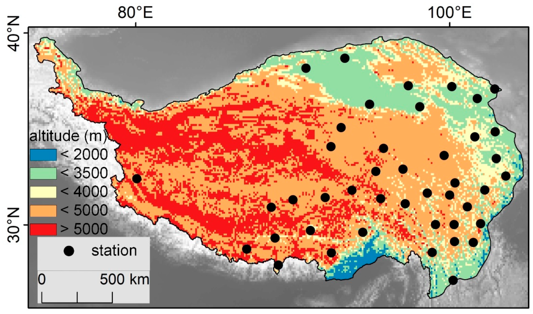
Air temperature data were collected from the National Climate Data Center, which is affiliated with the National Oceanic and Atmosphere Administration (NOAA) (Figure 1). These data were used to produce the average air temperature at different timescales from 1982 to 2013. First, we acquired 44 high-quality meteorological stations considering the geographical scope of the TP and the requirement of high-density temperature data. Second, we collected the daily mean temperature data for each station during 1982–2013 and replaced the missing values for a few of stations using the average air temperature of the neighboring days [32,33]. Finally, the mean temperature of annual and seasonal scales was calculated and used to detect trends and breakpoints in different warming phases of the TP.
2.2.2. Remote Sensing Products
The remote sensing data used in this study included the GIMMS and MODIS datasets. The GIMMS NDVI product (1982–2013) was derived from the AVHRR sensor of the National Oceanic and Atmospheric Administration (http://www.ncdc.noaa.gov/cdo-web, accessed on 3 October 2022), and it has a temporal resolution of 15 days and a spatial resolution of 8 km. The initial version of this dataset is not ideal for capturing vegetation dynamics, and therefore, the latest version mitigates this problem by correcting sensors, aerosols, and view geometry [34,35,36]. A maximum value composite procedure was used to remove some sources of interference, such as clouds, the atmosphere, and variation in solar altitude angle; after that, annual and seasonal NDVI values were obtained [37].
Compared to the AVHRR instrument, the updated MODIS instrument has a better sensitivity to chlorophyll with higher spatial resolution. We employed MODIS datasets of 2000–2021 including NDVI (MOD13A2), LST (MOD11A1), albedo (MCD43A3), and land cover types (MCD12Q1). Specifically, MOD13A2 and MOD11A1 have a 1 km spatial resolution and a 16-day temporal resolution. MOD11A1 and MCD43A3 were used in this study to better understand the relationships between LST and vegetation change. MCD12Q1 (version 6.1), providing annual land cover types (2001–2021), was also obtained to analyze the effect of land cover change on NDVI change trends. Additionally, all of the MODIS datasets were aggregated to 1 km to ensure the consistent spatial resolution of these datasets. We adopted different strategies in processing the MODIS-derived surface parameters by referring to previous studies. For each timescale, we processed the NDVI data using the maximum value composite method [37], and we processed the LST and albedo data using the mean value composite method [29,38].
2.3. Methods
Our analyses were performed in three major steps. Firstly, to analyze the NDVI responses at different warming phases, we performed breakpoint detection of air temperature data. Considering previous artificial temporal segmentation on NDVI variation [17,39,40,41], the Sequential Mann–Kendall (SQMK) [32,33,34,42] was employed to estimate the breakpoints of temperature change, and it was used as a proxy for classifying the different phases of NDVI responses. Please see the Supporting Information S1 for the detailed introduction to the SQMK test.
Secondly, we analyzed trends and performed a significance analysis [43,44] on key surface parameters. Sen’s slope estimator, a nonparametric test [45], was employed to determine trends in NDVI, LST, and albedo for different warming phases of all timescales. Please see the Supporting Information S2 for the detailed introduction to the Sen’s slope.
Thirdly, to identify the impacts of the NDVI on LST, both the detrending method and partial correlation analysis were performed among the NDVI, albedo, and LST. The purpose of using the detrending method was to eliminate any spurious correlations among the three parameters that may have been caused by temporal variations. As for the partial correlation analysis, it was used to better quantify the individual impact of NDVI or albedo on LST. The specific procedures included two aspects: (1) Using the first-difference detrending method (i.e., the difference of values in one year to the previous year), we examined and filtered the temporal trends of NDVI and albedo. (2) For partial correlation analysis, the partial correlation coefficient is an assessment of the net correlation between a single factor and the target value, provided that the impact of other factors is fixed or deducted. Considering the significant co-impact of vegetation and albedo on LST, the partial correlation coefficient is a good indicator for analyzing the relationship between them.
3. Results
3.1. Air Temperature and Vegetation Trends during 1982–2013 at Annual and Seasonal Scales
3.1.1. Annual Trends in Air Temperature and Vegetation
The air temperature and vegetation coverage on the TP generally increased on an annual scale (Figure 2a), while vegetation changes during each warming phase showed significant spatial and temporal variation. A significant abrupt change (p < 0.05) occurred in 1996 for air temperature trends on the TP (Figure 2b), and the warming trend during 1996–2013 (0.043 °C/year) was notably higher than that during 1982–1996 (0.042 °C/year), suggesting that the warming rate on the TP accelerated after 1996. The significant result (p < 0.05) revealed that the annual NDVI is generally increasing (Figure 2a) and the clustered NDVI increase and decrease in the second warming phase are greater than that in the first warming phase (Figure 2d,f). Specifically, the NDVI greened more than it browned during the first warming phase (Figure 2d), and there was clustered NDVI greening and browning in the eastern and western plateau (Figure 2f), respectively.
3.1.2. Seasonal Trends in Air Temperature and Vegetation
The air temperature and vegetation coverage on the TP during the spring seasons generally showed an increasing trend throughout the study period (Figure 3a). The breakpoint and warming rates were very different from those of the annual scale. The breakpoint for spring’s air temperature trend occurred in 1994, with a slope of 0.040 °C/year in the first warming phase and 0.034 °C/year in the second warming phase (Figure 3b), indicating that warming on the TP during the spring has slowed down. The NDVI showed a general increase over time, although the trend was more significant during the second warming phase (Figure 3c,e). Furthermore, the NDVI showed a significant increasing trend (p < 0.05) in the eastern TP and a significant decreasing trend in the northwestern part (Figure 3e). The significance statistics (p < 0.05) suggested that the clustered NDVI changes occurred in the second phase rather than in the first phase (Figure 3d,f). For example, TP NDVI decreased in the western part and increased in the eastern part (Figure 3f).
For summer, the TP exhibited both the largest NDVI value and the most significant warming trend (Figure 4a, p < 0.05), as did the largest pre- and post-phase difference in air temperature (Figure 4b). The breakpoint for the summer temperature on the TP occurred in 1998, which is slightly later than for the spring and annual scales. The trend for the second warming phase reached a rate of 0.047 °C/year, which is notably higher than that of the first warming phase. This implied that the warming rate in summer on the TP is much greater than that in other timescales. The significance analysis (p < 0.05) indicated that the NDVI increase is greater in the first warming phase than that in the second warming phase (Figure 4d,f), particularly in the western TP.
Autumn vegetation trends and warming both showed a lower value compared to the summer (Figure 5a). The breakpoint of temperature during the autumn occurred in 1994 (Figure 5b), similar to the spring. The first and second phases during autumn recorded trends of 0.029 °C/year and 0.018 °C/year, respectively. As such, the trend for the second phase was significantly weaker than that of the first phase, demonstrating that the warming rate on the TP becomes slow during autumn. The NDVI showed a non-significant fluctuation in general, and the significance statistics (p < 0.05) showed that the increase or decrease in the TP’s NDVI is less significant in the first phase than that in the second phase (Figure 5d,f), which is similar to the vegetation change pattern in spring.
The vegetation and air temperature changes on the TP documented during the winter were similar to those during the autumn, although they showed much smaller magnitudes than other timescales (Figure 6a,b). The breakpoint in the winter temperature between warming phases on the TP occurred in 1998; the trends of the first and second warming phases were 0.017 °C/year and 0.021 °C/year, respectively, indicating that the winter warming on the TP is accelerating (Figure 6b). Winter changes in the NDVI values were generally small. A fragmented NDVI increase occurred in the eastern TP of the first phase, but a massive NDVI decrease occurred in the second phase, which was not found for any other timescales (Figure 6d,f).
3.1.3. The Spatial and Temporal Responses of NDVI to Air Temperature
Our study identified consistent breakpoints in air temperature for spring and autumn as well as for summer and winter. We observed that the first warming phase showed a smaller trend than the second warming phase on most timescales. This suggests that while warming continues on the TP, the later warming trend is slightly decreasing.
We also investigated the spatial trends of NDVI at different warming phases. During the first warming phase, we found that the area of NDVI greening is smaller in spring and autumn with earlier breakpoints compared to summer and winter with later breakpoints. However, in the second warming phase, we observed that the area of NDVI increase is larger in spring and autumn with earlier breakpoints compared to summer and winter with later breakpoints. This indicates that the timescale with the earlier breakpoints exhibits a greater NDVI increase in the second warming phase. For instance, the air temperature breakpoint at the annual scale earlier than summer and winter showed a significantly larger area of NDVI increase in the second warming phase.
Furthermore, we found that in the relatively weaker second warming phase, there is more NDVI decrease at all timescales across the sparsely vegetated northwestern TP. This may be attributed to two factors: (1) limitations in the ability of the AVHRR sensor to capture detailed NDVI changes in sparsely vegetated areas, and (2) an increased vegetation sensitivity to air temperature during the second warming phase.
3.2. LST, Vegetation, and Albedo Trends during 2000–2021 at Annual and Seasonal Scales
3.2.1. LST Trends at Different Timescales
The spatial pattern of LST trends recorded at different timescales was more concentrated than that for the NDVI data. Alongside being common in winter, the LST warming trend on the TP from 2000 to 2021 was most prominent in the southern TP (Figure 7a–e). The LST warming rate was significantly higher in summer and autumn than during winter and spring, and it was mainly concentrated in the southwestern TP (Figure 7c,d). The LST cooling trend was most prominent on the northern TP on an annual scale and during spring, summer, and autumn (Figure 7a–d). During the winter, cooling mostly occurred in the southwestern TP. The spatial distribution of significance trends (p < 0.05) showed that the most significant decrease in LST occurs at annual scale and in spring (Figure 7f,j), with 7.06% and 7.93% of all pixels recording these changes, respectively. Significant LST increases (p < 0.05) in autumn were represented by 10.60% of all pixels (Figure 7i), which covered a much larger area than that for spring (5.01%; Figure 7g), summer (6.71%; Figure 7h), and winter (1.42%; Figure 7j).
3.2.2. NDVI Trends at Different Timescales
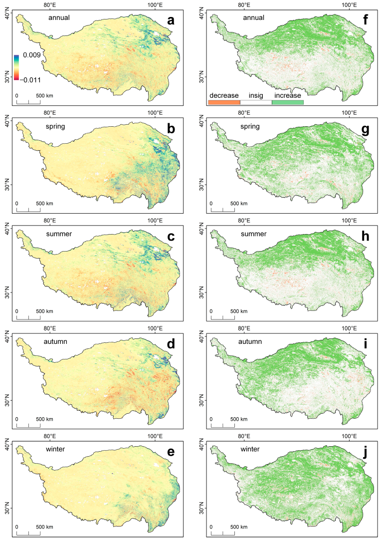
Spatial variations in the surface parameters across the study region revealed that MODIS-based NDVI data show significantly more greening trends than GIMMS-based NDVI data (Figure 8). These NDVI data showed that the eastern TP records the largest greening area during 2000–2021 at all timescales (Figure 8a–e), and the greening rate in the spring is significantly higher than for the other timescales (Figure 8b). The southern TP showed the highest NDVI browning rate (Figure 8a–d), which was highest in autumn out of all the considered timescales (Figure 8d). The NDVI data recorded an increasing trend on an annual scale, with 40.16% of pixels showing a significant increase and only 3.56% showing a significant decrease trend (Figure 8f, p < 0.05). Approximately 44.62% of the NDVI pixels showed a significant increase in the spring, and 2.53% significantly decreased (Figure 8g). Furthermore, 38.84% of the NDVI pixels showed significant greening (p < 0.05), and 3.49% showed a considerable browning during the summer (Figure 8h). An approximately equal proportion of NDVI pixels showed browning (21.13%) and greening (21.35%) in autumn (Figure 8i). Finally, 52.56% and 2.24% of the NDVI pixels recorded greening and browning in winter, respectively, with these values being significantly higher than their equivalents during the other seasons (Figure 8j).
3.2.3. Albedo Trends at Different Timescales
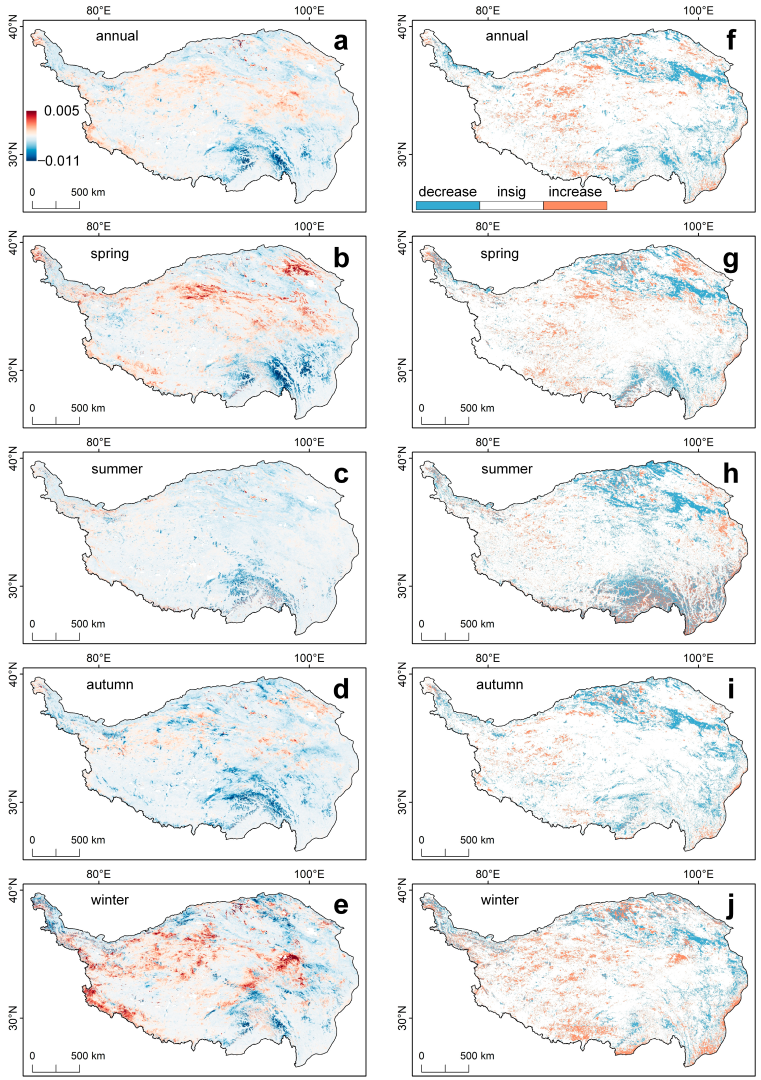
Albedo trends at all timescales showed relatively few spatial hotspots except for in winter (Figure 9a–e). The fastest albedo growth rates during 2000–2021 occurred in spring and winter (Figure 9b,e); however, the albedo trends in summer and autumn were less pronounced (Figure 9c,d). The decreasing rate of albedo was similar to its increasing rate in the temporal pattern. A significant increase in albedo was observed in the western plateau region at all timescales, and a significant decrease is found in the south and northeast plateau (Figure 9f–j, p < 0.05). In terms of areas distribution, a relatively high percentage of pixels showed a significant increase during spring (7.78%; Figure 9g) and winter (4.92%; Figure 9j), and they were notably higher than the values of 0.49% in summer and 0.38% in autumn. This effect may have been due to snow accumulation in spring and winter. The largest areas with significant decreasing trends in albedo were monitored in summer and autumn (Figure 9h,i, p < 0.05). These areas comprised 26.30% and 16.36% of the total number of pixels in the study region, respectively, and these changes might potentially be linked to increased vegetation coverage during the growing season.
3.2.4. Vegetation Impacts on LST at Different Time Scales
A statistical method was used to quantify the individual effect of vegetation on LST, and we simultaneously considered the varying albedo (see Section 3.2.3) due to its significant role in the vegetation–LST relationship [46,47]. Specifically, we employed the detrending method and partial correlation analysis to analyze the individual effects of the NDVI and albedo on LST. First, we examined the linear trends of the NDVI and albedo (see the Supporting Information S3 for details). The results suggested that the NDVI of the TP shows significant temporal trends at different timescales, and the summer albedo also shows significant temporal trends (Table 2). Consequently, we filtered the temporal trends of the indicated six variables using the detrending method. Second, we fixed NDVI (albedo) to analyze the correlation between albedo (NDVI) and LST. The results showed that the partial correlation coefficients of the NDVI and albedo with LST are significant except in summer (Table 3). This may be due to the saturation effect of the summer vegetation and albedo contributions on the LST [48], resulting in their insignificant trend of contribution. The individual contribution of albedo to LST was larger than that of NDVI at all timescales, especially in spring and autumn. This may be attributed to the fact that (1) the individual contribution of albedo to LST includes both the indirect contribution of vegetation altering albedo [49] and the direct contribution of albedo; and (2) an advanced vegetation growing season and a delayed vegetation ending season can alter surface albedo strongly [50,51], causing the contribution of surface albedo to be larger in spring and autumn. In terms of winter, faded vegetation and deepened snow cover would reduce the contribution of vegetation but increase the contribution of albedo [47].
Note that we utilized a statistical method to elucidate the relationship between vegetation, albedo, and LST, but we acknowledge its limitations due to the absence of a detailed surface radiation balance analysis. Achieving an accurate decomposition of surface radiation components would require further discussion beyond the scope and word limit of this paper. Therefore, for the purpose of this study, we considered the statistical method as a reasonable proxy for interpreting the individual impacts of vegetation and albedo on LST at various timescales. The individual impacts of vegetation and albedo to LST using surface radiative balance methods is expected in the near future. In addition, vegetation data are considered in producing LST products, yet it is difficult to estimate the contribution of vegetation data due to a lack of robust methods. Therefore, the vegetation contribution to LST estimation may have some uncertainties in the dense vegetation growth of the southeastern TP.
4. Discussion
Vegetation–temperature relationships can be affected by estimation methods, data sources, and land cover types. We therefore discussed the breakpoint method for vegetation trends, the differences between GIMMS and MODIS NDVI datasets, and the impacts of land cover types on annual NDVI trends.
Firstly, we analyzed vegetation–temperature relationships during different warming phases. In terms of methodology, the relationship between vegetation and climate variables on the TP presented remarkable phase changes. However, the phase division of such a relationship was usually subject to the limitation of the time span of remote sensing observed vegetation datasets and the study period. For example, a 5-year time step was used to investigate the relationship between climatic and non-climatic factors and vegetation on the TP during 1980–2010 [40], and a visual graphical approach was used to determine the breakpoints in TP vegetation during 1982–2002 [41] as well as artificial time segmentation to investigate the TP vegetation feedback to climatic factors [39,46]. These methods may lead to bias in the vegetation response analysis. We therefore used the breakpoints in temperature change as the reference time points when analyzing the TP vegetation changes at different phases. We found that the breakpoints of TP temperature during 1982–2013 at different time scales largely occurred between 1994 and 1998 (Figure 2, Figure 3, Figure 4, Figure 5 and Figure 6). This result is not only closer to direct NDVI segmentation investigation on the TP [52], but it is also closer to the artificial breakpoint of 2000 years in some investigations of TP NDVI response analysis [39,46]. Nevertheless, our results strongly imply that the artificial abrupt points later than 2000 may bring greater bias in TP NDVI response analysis. Our study also found that a common warming trend occurred at all timescales during 1982–2013, and the breakpoints of the TP were earlier in spring and autumn than those annually and in the summer and winter (Figure 2, Figure 3, Figure 4, Figure 5 and Figure 6). This indicates that the growth and end season of vegetation may advance the warming breakpoint of the TP [50]. With the TP warming, the second phase of NDVI increase was significant at all timescales except winter, implying potential temperature accumulation induced by the first warming phase contributing to the vegetation growth in the second phase.
Secondly, our investigation demonstrated a significant NDVI trend difference between the GIMMS and MODIS datasets. Overall, NDVI trends were greater in MODIS data than in GIMMS, and this finding was consistent with [46,53]. The GIMMS NDVI data did not show a significant increase in 2000–2013, which was also found in [46,54]. This may be attributed to the wider NIR band [55] and the imperfect atmospheric effects processing technique for GIMMS data [56]. Fortunately, MODIS data are usually more reliable than GIMMS data and fill the GIMMS data gap well [57]. For example, our results indicated a significant increase in MODIS NDVI trends during 2000–2021 (Figure 8). Nevertheless, both GIMMS and MODIS products showed a common trend of vegetation changes on the TP (Figure 3a and Figure 8a). However, given the advantages of the long time series of GIMMS data and the moderate accuracy of MODIS data, it is of great significance to integrate multiple datasets to analyze the future vegetation and climatic factors on the TP.
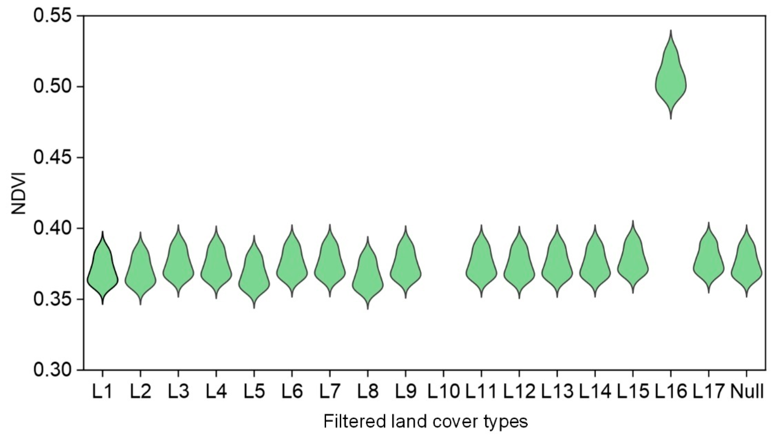
Thirdly, given the recent warm and wet trends on the TP [31,58], we further estimated the relative impact of NDVI changes in different land cover types on annual NDVI trend on the TP. Based on the MODIS land cover product, we detected annual land cover data in 2001 and 2021 and produced change pixels and unchanged land cover types on the TP. The results showed that 89% of the land cover types on the TP have remained unchanged over the 2001–2021 period (Figure 10). Given that the unchanged pixels cover the majority of the TP, a stepwise backward method based on these areas was employed to filter the intended land cover types and then evaluate their relative impact on the estimation of NDVI trends of TP. The results suggested that only bare land has a relative impact of 9.746% on the TP NDVI trend, but the relative impact of other land cover types on the TP NDVI trend does not exceed 5% (Table 4). This implied that the NDVI growth of bare land contributes significantly to the TP vegetation. In addition, we also found that the mean NDVI value of the TP reaches the highest after filtering the bare land compared to other cover types (Figure 11). Accordingly, we suggest that future NDVI trend and intensity studies on the TP should pay more attention to vegetation changes in bare land.
5. Conclusions
This study aimed to investigate the differences in vegetation changes during various warming phases on the Tibetan Plateau (TP) as well as the trends and patterns of NDVI at different timescales and its influence on LST over the past two decades. First, the warming trend on the TP occurred at different timescales, corresponding to breakpoints that took place in 1994–1998, with earlier occurrences observed in spring and autumn. Secondly, as the warming of the TP continued, the vegetation in the second warming phase exhibited a larger greening area. These findings suggested that the time of temperature breakpoints may have an impact on the area of vegetation increase, and NDVI changes are more sensitive to air temperature during the recent warming phase. Third, MODIS data highlighted more greening compared to GIMMS data. Using MODIS data, we also found the fastest NDVI increase trend in spring and the fastest LST warming in autumn. The partial correlation analysis indicated that NDVI has a significant negative impact on LST during the annual scale and autumn while also having a significant positive impact on LST during spring. This suggests that the contribution of NDVI to LST varies across different timescales since 2000. To summarize, our findings systematically uncover the spatiotemporal patterns of air temperature, LST, and NDVI on the TP across different timescales. These results provide significant insights into the annual and seasonal patterns of vegetation responses and feedback to climate change on the TP. Furthermore, our analysis reveals distinct seasonal trends between NDVI and LST, which can be leveraged to enhance the accuracy of numerical simulations that aim to replicate the relationships between vegetation and climate over the TP.
Supplementary Materials
The following supporting information can be downloaded at: https://www.mdpi.com/article/10.3390/rs15092475/s1, Section S1: Detailed procedures of SQMK test; Section S2: Detailed procedures of Sen’s slope; Section S3: Overall trends of NDVI, LST, and albedo over the Tibetan Plateau (Figure S1: MODIS-based NDVI, LST, and albedo trends over the Tibetan Plateau at annual and seasonal scales during 2000–2021) [59,60].
Author Contributions
Conceptualization, F.W. and Y.M.; methodology, F.W.; manuscript, F.W. and Y.M.; funding acquisition, Y.M. Writing—review and editing, F.W., Y.M., R.D. and C.H.; All authors have read and agreed to the published version of the manuscript.
Funding
This research was funded by the Second Tibetan Plateau Scientific Expedition and Research (STEP) program (2019QZKK0103) and the National Natural Science Foundation of China (42230610 and 91837208).
Data Availability Statement
All input data for this research are publicly available: global inventory modeling and mapping studies (GIMMS) NDVI data (https://climatedataguide.ucar.edu/climate-data/ndvi-normalized-difference-vegetation-index-3rd-generation-nasagfsc-gimms), moderate-resolution imaging spectroradiometer (MODIS) NDVI data (https://lpdaac.usgs.gov/products/mod13a2v061), moderate-resolution imaging spectroradiometer (MODIS) LST data (https://lpdaac.usgs.gov/products/mod11a2v061), moderate-resolution imaging spectroradiometer (MODIS) albedo data (https://lpdaac.usgs.gov/products/mcd43a3v061), moderate-resolution imaging spectroradiometer (MODIS) Land Cover Type data (https://lpdaac.usgs.gov/products/mcd12q1v061), and surface-near air temperature (https://www.ncdc.noaa.gov/cdo-web).
Acknowledgments
The author would like to acknowledge all the members of the Land–Atmosphere Interaction and Its Climatic Effects Group. We also thank reviewers for their valuable comments and the China Scholarship Council (CSC).
Conflicts of Interest
The authors declare no conflict of interest.
References
- Gerten, D.; Schaphoff, S.; Haberlandt, U.; Lucht, W.; Sitch, S. Terrestrial vegetation and water balance—Hydrological evaluation of a dynamic global vegetation model. J. Hydrol. 2004, 286, 249–270. [Google Scholar] [CrossRef]
- Zuo, Z.; Zhang, R.; Zhao, P. The relation of vegetation over the Tibetan Plateau to rainfall in China during the boreal summer. Clim. Dyn. 2011, 36, 1207–1219. [Google Scholar] [CrossRef]
- Piao, S.; Wang, X.; Park, T.; Chen, C.; Lian, X.; He, Y.; Bjerke, J.W.; Chen, A.; Ciais, P.; Tømmervik, H.; et al. Characteristics, drivers and feedbacks of global greening. Nat. Rev. Earth Environ. 2020, 1, 14–27. [Google Scholar] [CrossRef]
- Forzieri, G.; Alkama, R.; Miralles, D.G.; Cescatti, A. Satellites reveal contrasting responses of regional climate to the widespread greening of Earth. Science 2017, 356, 1180–1184. [Google Scholar] [CrossRef] [PubMed]
- Zeng, Z.; Piao, S.; Li, L.Z.X.; Zhou, L.; Ciais, P.; Wang, T.; Li, Y.; Lian, X.; Wood, E.F.; Friedlingstein, P.; et al. Climate mitigation from vegetation biophysical feedbacks during the past three decades. Nat. Clim. Chang. 2017, 7, 432–436. [Google Scholar] [CrossRef]
- Zhong, L.; Ma, Y.; Xue, Y.; Piao, S. Climate Change Trends and Impacts on Vegetation Greening over the Tibetan Plateau. J. Geophys. Res. Atmos. 2019, 124, 7540–7552. [Google Scholar] [CrossRef]
- Yu, H.; Luedeling, E.; Xu, J. Winter and spring warming result in delayed spring phenology on the Tibetan Plateau. Proc. Natl. Acad. Sci. USA 2010, 107, 22151–22156. [Google Scholar] [CrossRef]
- Zhou, H.K.; Yao, B.Q.; Xu, W.X.; Ye, X.; Fu, J.J.; Jin, Y.X.; Zhao, X.Q. Field evidence for earlier leaf-out dates in alpine grassland on the eastern Tibetan Plateau from 1990 to 2006. Biol. Lett. 2014, 10, 20140291. [Google Scholar] [CrossRef]
- Ding, M.; Zhang, Y.; Liu, L.; Zhang, W.; Wang, Z.; Bai, W. The relationship between NDVI and precipitation on the Tibetan Plateau. J. Geogr. Sci. 2007, 17, 259–268. [Google Scholar] [CrossRef]
- Pang, G.; Wang, X.; Yang, M. Using the NDVI to identify variations in, and responses of, vegetation to climate change on the Tibetan Plateau from 1982 to 2012. Quat. Int. 2017, 444, 87–96. [Google Scholar] [CrossRef]
- Duan, A.; Wu, G.; Liu, Y.; Ma, Y.; Zhao, P. Weather and climate effects of the Tibetan Plateau. Adv. Atmos. Sci. 2012, 29, 978–992. [Google Scholar] [CrossRef]
- Latif, A.; Ilyas, S.; Zhang, Y.; Xin, Y.; Zhou, L.; Zhou, Q. Review on global change status and its impacts on the Tibetan Plateau environment. J. Plant Ecol. 2019, 12, 917–930. [Google Scholar] [CrossRef]
- Li, Y.; Zhao, M.; Motesharrei, S.; Mu, Q.; Kalnay, E.; Li, S. Local cooling and warming effects of forests based on satellite observations. Nat. Commun. 2015, 6, 6603. [Google Scholar] [CrossRef] [PubMed]
- Verrelst, J.; Camps-Valls, G.; Muñoz-Marí, J.; Rivera, J.P.; Veroustraete, F.; Clevers, J.G.P.W.; Moreno, J. Optical remote sensing and the retrieval of terrestrial vegetation bio-geophysical properties—A review. ISPRS J. Photogramm. Remote Sens. 2015, 108, 273–290. [Google Scholar] [CrossRef]
- Bright, R.M.; Davin, E.; O’halloran, T.; Pongratz, J.; Zhao, K.; Cescatti, A. Local temperature response to land cover and management change driven by non-radiative processes. Nat. Clim. Chang. 2017, 7, 296–302. [Google Scholar] [CrossRef]
- Ge, J.; Guo, W.; Pitman, A.J.; De Kauwe, M.G.; Chen, X.; Fu, C. The Nonradiative Effect Dominates Local Surface Temperature Change Caused by Afforestation in China. J. Clim. 2019, 32, 4445–4471. [Google Scholar] [CrossRef]
- Shen, M.; Piao, S.; Jeong, S.-J.; Zhou, L.; Zeng, Z.; Ciais, P.; Chen, D.; Huang, M.; Jin, C.-S.; Li, L.Z.X.; et al. Evaporative cooling over the Tibetan Plateau induced by vegetation growth. Proc. Natl. Acad. Sci. USA 2015, 112, 9299–9304. [Google Scholar] [CrossRef]
- Zhong, L.; Ma, Y.; Salama, M.S.; Su, Z. Assessment of vegetation dynamics and their response to variations in precipitation and temperature in the Tibetan Plateau. Clim. Chang. 2010, 103, 519–535. [Google Scholar] [CrossRef]
- Huete, A.R.; Liu, H.Q.; Batchily, K.V.; van Leeuwen, W. A comparison of vegetation indices over a global set of TM images for EOS-MODIS. Remote Sens. Environ. 1997, 59, 440–451. [Google Scholar] [CrossRef]
- Piao, S.; Fang, J.; Liu, H.; Zhu, B. NDVI-indicated decline in desertification in China in the past two decades. Geophys. Res. Lett. 2005, 32, L06402. [Google Scholar] [CrossRef]
- Yuan-He, Y.; Shi-Long, P. Variations in grassland vegetation cover in relation to climatic factors on the Tibetan Plateau. Chin. J. Plant Ecol. 2006, 30, 1–8. [Google Scholar] [CrossRef]
- Lin, X.; Wen, J.; Liu, Q.; You, D.; Wu, S.; Hao, D.; Xiao, Q.; Zhang, Z.; Zhang, Z. Spatiotemporal Variability of Land Surface Albedo over the Tibet Plateau from 2001 to 2019. Remote Sens. 2020, 12, 1188. [Google Scholar] [CrossRef]
- Guo, D.; Sun, J.; Yang, K.; Pepin, N.; Xu, Y.; Xu, Z.; Wang, H. Satellite data reveal southwestern Tibetan plateau cooling since 2001 due to snow-albedo feedback. Int. J. Clim. 2020, 40, 1644–1655. [Google Scholar] [CrossRef]
- Salama, M.S.; Van Der Velde, R.; Zhong, L.; Ma, Y.; Ofwono, M.; Su, Z. Decadal variations of land surface temperature anomalies observed over the Tibetan Plateau by the Special Sensor Microwave Imager (SSM/I) from 1987 to 2008. Clim. Chang. 2012, 114, 769–781. [Google Scholar] [CrossRef]
- Luo, D.L.; Jin, H.J.; He, R.X.; Wang, X.F.; Muskett, R.R.; Marchenko, S.S.; Romanovsky, V.E. Characteristics of Water-Heat Exchanges and Inconsistent Surface Temperature Changes at an Elevational Permafrost Site on the Qinghai-Tibet Plateau. J. Geophys. Res. Atmos. 2018, 123, 10057–10075. [Google Scholar] [CrossRef]
- Stroppiana, D.; Antoninetti, M.; Brivio, P.A. Seasonality of MODIS LST over Southern Italy and correlation with land cover, topography and solar radiation. Eur. J. Remote Sens. 2014, 47, 133–152. [Google Scholar] [CrossRef]
- Zhou, Y.; Ran, Y.; Li, X. The contributions of different variables to elevation-dependent land surface temperature changes over the Tibetan Plateau and surrounding regions. Glob. Planet. Chang. 2023, 220, 104010. [Google Scholar] [CrossRef]
- Zhu, W.; Lű, A.; Jia, S. Estimation of daily maximum and minimum air temperature using MODIS land surface temperature products. Remote Sens. Environ. 2013, 130, 62–73. [Google Scholar] [CrossRef]
- Yang, M.; Zhao, W.; Zhan, Q.; Xiong, D. Spatiotemporal Patterns of Land Surface Temperature Change in the Tibetan Plateau Based on MODIS/Terra Daily Product From 2000 to 2018. IEEE J. Sel. Top. Appl. Earth Obs. Remote Sens. 2021, 14, 6501–6514. [Google Scholar] [CrossRef]
- Yang, K.; Wu, H.; Qin, J.; Lin, C.; Tang, W.; Chen, Y. Recent climate changes over the Tibetan Plateau and their impacts on energy and water cycle: A review. Glob. Planet. Chang. 2014, 112, 79–91. [Google Scholar] [CrossRef]
- Li, L.; Yang, S.; Wang, Z.; Zhu, X.; Tang, H. Evidence of Warming and Wetting Climate over the Qinghai-Tibet Plateau. Arct. Antarct. Alp. Res. 2010, 42, 449–457. [Google Scholar] [CrossRef]
- Zhang, Q.; Singh, V.P.; Li, J.; Chen, X. Analysis of the periods of maximum consecutive wet days in China. J. Geophys. Res. Atmos. 2011, 116, D23106. [Google Scholar] [CrossRef]
- Guan, Y.; Zheng, F.; Zhang, X.; Wang, B. Trends and variability of daily precipitation and extremes during 1960–2012 in the Yangtze River Basin, China. Int. J. Clim. 2017, 37, 1282–1298. [Google Scholar] [CrossRef]
- Bachelet, D.; Neilson, R.P.; Lenihan, J.M.; Drapek, R.J. Climate Change Effects on Vegetation Distribution and Carbon Budget in the United States. Ecosystems 2001, 4, 164–185. [Google Scholar] [CrossRef]
- Ma, M.; Frank, V. Interannual variability of vegetation cover in the Chinese Heihe River Basin and its relation to meteorological parameters. Int. J. Remote Sens. 2006, 27, 3473–3486. [Google Scholar] [CrossRef]
- Anyamba, A.; Small, J.L.; Tucker, C.J.; Pak, E.W. Thirty-two Years of Sahelian Zone Growing Season Non-Stationary NDVI3g Patterns and Trends. Remote Sens. 2014, 6, 3101–3122. [Google Scholar] [CrossRef]
- Holben, B.N. Characteristics of maximum-value composite images from temporal AVHRR data. Int. J. Remote Sens. 1986, 7, 1417–1434. [Google Scholar] [CrossRef]
- Zheng, L.; Qi, Y.; Qin, Z.; Xu, X.; Dong, J. Assessing albedo dynamics and its environmental controls of grasslands over the Tibetan Plateau. Agric. For. Meteorol. 2021, 307, 108479. [Google Scholar] [CrossRef]
- Du, J.; Zhao, C.; Shu, J.; Jiaerheng, A.; Yuan, X.; Yin, J.; Fang, S.; He, P. Spatiotemporal changes of vegetation on the Tibetan Plateau and relationship to climatic variables during multiyear periods from 1982–2012. Environ. Earth Sci. 2015, 75, 77. [Google Scholar] [CrossRef]
- Pan, T.; Zou, X.; Liu, Y.; Wu, S.; He, G. Contributions of climatic and non-climatic drivers to grassland variations on the Tibetan Plateau. Ecol. Eng. 2017, 108, 307–317. [Google Scholar] [CrossRef]
- Zhou, D.; Fan, G.; Huang, R.; Fang, Z.; Liu, Y.; Li, H. Interannual variability of the normalized difference vegetation index on the Tibetan Plateau and its relationship with climate change. Adv. Atmos. Sci. 2007, 24, 474–484. [Google Scholar] [CrossRef]
- Wang, X.; Xiao, J.; Li, X.; Cheng, G.; Ma, M.; Che, T.; Dai, L.; Wang, S.; Wu, J. No Consistent Evidence for Advancing or Delaying Trends in Spring Phenology on the Tibetan Plateau. J. Geophys. Res. Biogeosci. 2017, 122, 3288–3305. [Google Scholar] [CrossRef]
- McLeod, A.I. Kendall rank correlation and Mann-Kendall trend test. R Package Kendall 2005, 602, 1–10. Available online: https://cran.r-project.org/web/packages/Kendall/index.html (accessed on 5 April 2023).
- Mann, H.B. Nonparametric tests against trend. Econometrica 1945, 13, 245–259. [Google Scholar] [CrossRef]
- Sen, P.K. Estimates of the regression coefficient based on Kendall’s Tau. J. Am. Stat. Assoc. 1968, 63, 1379–1389. [Google Scholar] [CrossRef]
- Querin, C.A.S.; Beneditti, C.A.; Machado, N.G.; da Silva, M.J.G.; da Silva Querino, K.A.; dos Santos Neto, L.A.; Biudes, M.S. Spatiotemporal NDVI, LAI, albedo, and surface temperature dynamics in the southwest of the Brazilian Amazon forest. J. Appl. Remote Sens. 2016, 10, 026007. [Google Scholar] [CrossRef]
- Pang, G.; Chen, D.; Wang, X.; Lai, H.-W. Spatiotemporal variations of land surface albedo and associated influencing factors on the Tibetan Plateau. Sci. Total. Environ. 2022, 804, 150100. [Google Scholar] [CrossRef]
- Lian, X.; Jiao, L.; Liu, Z. Saturation response of enhanced vegetation productivity attributes to intricate interactions. Glob. Chang. Biol. 2023, 29, 1080–1095. [Google Scholar] [CrossRef]
- Tian, L.; Zhang, Y.; Zhu, J. Decreased surface albedo driven by denser vegetation on the Tibetan Plateau. Environ. Res. Lett. 2014, 9, 104001. [Google Scholar] [CrossRef]
- Shen, M.; Zhang, G.; Cong, N.; Wang, S.; Kong, W.; Piao, S. Increasing altitudinal gradient of spring vegetation phenology during the last decade on the Qinghai-Tibetan Plateau. Agric. For. Meteorol. 2014, 189–190, 71–80. [Google Scholar] [CrossRef]
- Du, J.; He, P.; Fang, S.; Liu, W.; Yuan, X.; Yin, J. Autumn NDVI contributes more and more to vegetation improvement in the growing season across the Tibetan Plateau. Int. J. Digit. Earth 2017, 10, 1098–1117. [Google Scholar] [CrossRef]
- Wang, Z.; Wang, Q.; Wu, X.; Zhao, L.; Yue, G.; Nan, Z.; Wang, P.; Yi, S.; Zou, D.; Qin, Y.; et al. Vegetation Changes in the Permafrost Regions of the Qinghai-Tibetan Plateau from 1982–2012: Different Responses Related to Geographical Locations and Vegetation Types in High-Altitude Areas. PLoS ONE 2017, 12, e0169732. [Google Scholar] [CrossRef] [PubMed]
- Liu, L.; Wang, Y.; Wang, Z.; Li, D.; Zhang, Y.; Qin, D.; Li, S. Elevation-dependent decline in vegetation greening rate driven by increasing dryness based on three satellite NDVI datasets on the Tibetan Plateau. Ecol. Indic. 2019, 107, 105569. [Google Scholar] [CrossRef]
- Zhang, G.; Zhang, Y.; Dong, J.; Xiao, X. Green-up dates in the Tibetan Plateau have continuously advanced from 1982 to 2011. Proc. Natl. Acad. Sci. USA 2013, 110, 4309–4314. [Google Scholar] [CrossRef] [PubMed]
- Guo, X.; Zhang, H.; Wu, Z.; Zhao, J.; Zhang, Z. Comparison and Evaluation of Annual NDVI Time Series in China Derived from the NOAA AVHRR LTDR and Terra MODIS MOD13C1 Products. Sensors 2017, 17, 1298. [Google Scholar] [CrossRef] [PubMed]
- Donohue, R.J.; Roderick, M.L.; McVicar, T.R. Deriving consistent long-term vegetation information from AVHRR reflectance data using a cover-triangle-based framework. Remote Sens. Environ. 2008, 112, 2938–2949. [Google Scholar] [CrossRef]
- Beck, P.S.; Goetz, S.J. Satellite observations of high northern latitude vegetation productivity changes between 1982 and 2008: Ecological variability and regional differences. Environ. Res. Lett. 2011, 6, 045501. [Google Scholar] [CrossRef]
- Wang, J.; Chen, X.; Hu, Q.; Liu, J. Responses of terrestrial water storage to climate variation in the Tibetan Plateau. J. Hydrol. 2020, 584, 124652. [Google Scholar] [CrossRef]
- Hussain, A.; Cao, J.; Ali, S.; Ullah, W.; Muhammad, S.; Hussain, I.; Rezaei, A.; Hamal, K.; Akhtar, M.; Abbas, H.; et al. Variability in Runoff and Responses to Land and Oceanic Parameters in the Source Region of the Indus River. Ecol. Indicators 2022, 140, 109014. [Google Scholar] [CrossRef]
- Ullah, S.; You, Q.; Ullah, W.; Ali, A. Observed Changes in Precipitation in China-Pakistan Economic Corridor during 1980–2016. Atmos. 2018, 210, 1–14. [Google Scholar] [CrossRef]
Figure 1.
Location of meteorological stations on the Tibetan Plateau.

Figure 2.
Vegetation and air temperature trends on the annual scale. GIMMS-based NDVI and air temperature trends during 1982–2013 (a); air temperature breakpoint detection based on the MK method (b). In (b), the gray dashed line denotes the detected temperature breakpoint, and UF and UB refer to the statistics of forward and backward sequence, respectively; GIMMS-based NDVI trends (c) and regions of significant change (d) during the first warming phase; GIMMS-based NDVI trends (e) and regions of significant change (f) during the second warming phase.

Figure 3.
Vegetation and air temperature trends in spring. GIMMS-based NDVI and air temperature trends during 1982–2013 (a); air temperature breakpoint detection based on the MK method (b). In (b), the gray dashed line denotes the detected temperature breakpoint, and UF and UB refer to the statistics of forward and backward sequence, respectively; GIMMS-based NDVI trends (c) and regions of significant change (d) during the first warming phase. GIMMS-based NDVI trends (e) and regions of significant change (f) during the second warming phase.

Figure 4.
Vegetation and air temperature trends in summer. GIMMS-based NDVI and air temperature trends during 1982–2013 (a); air temperature breakpoint detection based on the MK method (b). In (b), the gray dashed line denotes the detected temperature breakpoint, and UF and UB refer to the statistics of forward and backward sequence, respectively; GIMMS-based NDVI trends (c) and regions of significant change (d) during the first warming phase. GIMMS-based NDVI trends (e) and regions of significant change (f) during the second warming phase.

Figure 5.
Vegetation and air temperature trends in autumn. GIMMS-based NDVI and air temperature trends during 1982–2013 (a); air temperature breakpoint detection based on the MK method (b). In (b), the gray dashed line denotes the detected temperature breakpoint, and UF and UB refer to the statistics of forward and backward sequence, respectively; GIMMS-based NDVI trends (c) and regions of significant change (d) during the first warming phase. GIMMS-based NDVI trends (e) and regions of significant change (f) during the second warming phase.

Figure 6.
Vegetation and air temperature trends in winter. GIMMS-based NDVI and air temperature trends during 1982–2013 (a); air temperature breakpoint detection based on the MK method (b). In (b), the gray dashed line denotes the detected temperature breakpoint, and UF and UB refer to the statistics of forward and backward sequence, respectively; GIMMS-based NDVI trends (c) and regions of significant change (d) during the first warming phase. GIMMS-based NDVI trends (e) and regions of significant change (f) during the second warming phase.

Figure 7.
MODIS-based LST trends during 2000–2021 at annual and seasonal scales. (a–e) denote the LST trends for 2000–2021 in annual, spring, summer, autumn, and winter, respectively; (f–j) denote the LST trends with p < 0.05 for 2000–2021 in annual, spring, summer, autumn, and winter, respectively.

Figure 8.
MODIS-based NDVI trends during 2000–2021 at annual and seasonal scales. (a–e) denote the NDVI trends for 2000–2021 in annual, spring, summer, autumn, and winter, respectively; (f–j) denote the NDVI trends with p < 0.05 for 2000–2021 in annual, spring, summer, autumn, and winter, respectively.

Figure 9.
MODIS-based albedo trends during 2000–2021 at annual and seasonal scales. (a–e) denote the albedo trends for 2000–2021 in annual, spring, summer, autumn, and winter, respectively; (f–j) denote the albedo trends with p < 0.05 for 2000–2021 in annual, spring, summer, autumn, and winter, respectively.

Figure 10.
Land cover change detection on the Tibetan Plateau during 2001–2021.

Figure 11.
Mean NDVI distribution for 2000–2021 after removing different land cover types. L1, L2, L3, L4, L5, L6, L7, L8, L9, L10, L11, L12, L13, L14, L15, L16, and L17 represent evergreen needleleaf forests, evergreen broadleaf forests, deciduous needleleaf forests, deciduous broadleaf forests, mixed forests, closed shrublands, open shrublands, woody savannas, savannas, grasslands, permanent wetlands, croplands, urban and built-up lands, cropland/natural vegetation, mosaics, permanent snow and ice, barren, and water bodies, respectively. Null means no filtered land cover type.


Table 1.
Data sources used in this study.
| Parameter | Dataset | Spatial Resolution | Temporal Resolution | Download Links |
|---|---|---|---|---|
| GIMMS NDVI | Version 5 | 8 km | 15 days | https://climatedataguide.ucar.edu/climate-data/ndvi-normalized-difference-vegetation-index-3rd-generation-nasagfsc-gimms, accessed on 3 October 2022 |
| Normalized difference vegetation index (NDVI) | MOD13A2 | 1000 m | 16 days | https://lpdaac.usgs.gov/products/mod13a2v061, accessed on 3 October 2022 |
| Land surface temperature (LST) | MOD11A1 | 1000 m | 8 days | https://lpdaac.usgs.gov/products/mod11a2v061, accessed on 3 October 2022 |
| Albedo | MCD43A3 | 500 m | daily | https://lpdaac.usgs.gov/products/mcd43a3v061, accessed on 3 October 2022 |
| Land Cover Type | MCD12Q1 | 500 m | yearly | https://lpdaac.usgs.gov/products/mcd12q1v061, accessed on 3 October 2022 |
| Air temperature | / | / | monthly | https://www.ncdc.noaa.gov/cdo-web, accessed on 3 October 2022 |
Table 2.
Significance of temporal trends in NDVI and albedo over 2000–2021.
| Independent Variables | R2 | F-Test | Sig. |
|---|---|---|---|
| MODIS-based annual NDVI | 0.628 | 33.729 | 0.000 |
| MODIS-based spring NDVI | 0.437 | 15.509 | 0.001 |
| MODIS-based summer NDVI | 0.581 | 27.779 | 0.000 |
| MODIS-based autumn NDVI | 0.412 | 14.040 | 0.001 |
| MODIS-based winter NDVI | 0.567 | 26.174 | 0.000 |
| MODIS-based annual albedo | 0.000 | 0.004 | 0.950 |
| MODIS-based spring albedo | 0.008 | 0.156 | 0.697 |
| MODIS-based summer albedo | 0.490 | 19.188 | 0.000 |
| MODIS-based autumn albedo | 0.030 | 0.608 | 0.445 |
| MODIS-based winter albedo | 0.050 | 1.061 | 0.315 |
| MODIS-based annual NDVI | 0.628 | 33.729 | 0.000 |
Table 3.
Partial correlation coefficients and significance of NDVI (albedo) with LST after fixing for albedo (NDVI).
Table 3.
Partial correlation coefficients and significance of NDVI (albedo) with LST after fixing for albedo (NDVI).
| MODIS-Based LST | MODIS-Based NDVI | MODIS-Based Albedo | ||
|---|---|---|---|---|
| Partial Correlation Coefficient | Two-Tailed Test | Partial Correlation Coefficient | Two-Tailed Test | |
| annual | −0.478 | 0.028 | −0.603 | 0.004 |
| spring | 0.467 | 0.033 | −0.856 | 0.000 |
| summer | −0.283 | 0.214 | −0.277 | 0.223 |
| autumn | −0.436 | 0.048 | −0.883 | 0.000 |
| winter | 0.041 | 0.858 | −0.803 | 0.000 |
Table 4.
Relative impact of land cover on annual NDVI trends on the Tibetan Plateau.
| Filtered Land Cover | Trend | R2 | Sig. | Relative Impact (%) |
|---|---|---|---|---|
| Evergreen Needleleaf Forests | 10.839 | 0.625 | 0.000 | 0.324 |
| Evergreen Broadleaf Forests | 10.826 | 0.624 | 0.000 | 0.204 |
| Deciduous Needleleaf Forests | 10.804 | 0.628 | 0.000 | 0.000 |
| Deciduous Broadleaf Forests | 10.798 | 0.627 | 0.000 | 0.056 |
| Mixed Forests | 10.828 | 0.622 | 0.000 | 0.222 |
| Closed Shrublands | 10.804 | 0.628 | 0.000 | 0.000 |
| Open Shrublands | 10.814 | 0.628 | 0.000 | 0.093 |
| Woody Savannas | 10.785 | 0.621 | 0.000 | 0.176 |
| Savannas | 10.782 | 0.626 | 0.000 | 0.204 |
| Grasslands | 10.986 | 0.883 | 0.000 | 1.685 |
| Permanent Wetlands | 10.802 | 0.628 | 0.000 | 0.019 |
| Croplands | 10.787 | 0.628 | 0.000 | 0.157 |
| Urban and Built-Up Lands | 10.809 | 0.628 | 0.000 | 0.046 |
| Cropland/Natural Vegetation Mosaics | 10.804 | 0.628 | 0.000 | 0.000 |
| Permanent Snow and Ice | 10.834 | 0.625 | 0.000 | 0.278 |
| Barren | 11.857 | 0.518 | 0.000 | 9.746 |
| Water Bodies | 10.293 | 0.599 | 0.000 | 4.730 |
| Null | 10.804 | 0.628 | 0.000 | / |
Notes: Null means no filtered land cover type.
Disclaimer/Publisher’s Note: The statements, opinions and data contained in all publications are solely those of the individual author(s) and contributor(s) and not of MDPI and/or the editor(s). MDPI and/or the editor(s) disclaim responsibility for any injury to people or property resulting from any ideas, methods, instructions or products referred to in the content. |
© 2023 by the authors. Licensee MDPI, Basel, Switzerland. This article is an open access article distributed under the terms and conditions of the Creative Commons Attribution (CC BY) license (https://creativecommons.org/licenses/by/4.0/).
Share and Cite
MDPI and ACS Style
Wang, F.; Ma, Y.; Darvishzadeh, R.; Han, C. Annual and Seasonal Trends of Vegetation Responses and Feedback to Temperature on the Tibetan Plateau since the 1980s. Remote Sens. 2023, 15, 2475. https://doi.org/10.3390/rs15092475
AMA Style
Wang F, Ma Y, Darvishzadeh R, Han C. Annual and Seasonal Trends of Vegetation Responses and Feedback to Temperature on the Tibetan Plateau since the 1980s. Remote Sensing. 2023; 15(9):2475. https://doi.org/10.3390/rs15092475
Chicago/Turabian StyleWang, Fangfang, Yaoming Ma, Roshanak Darvishzadeh, and Cunbo Han. 2023. "Annual and Seasonal Trends of Vegetation Responses and Feedback to Temperature on the Tibetan Plateau since the 1980s" Remote Sensing 15, no. 9: 2475. https://doi.org/10.3390/rs15092475
Note that from the first issue of 2016, this journal uses article numbers instead of page numbers. See further details here.