Self-Adaptive-Filling Deep Convolutional Neural Network Classification Method for Mountain Vegetation Type Based on High Spatial Resolution Aerial Images

Abstract

The composition and structure of mountain vegetation are complex and changeable, and thus urgently require the integration of Object-Based Image Analysis (OBIA) and Deep Convolutional Neural Networks (DCNNs). However, while integration technology studies are continuing to increase, there have been few studies that have carried out the classification of mountain vegetation by combining OBIA and DCNNs, for it is difficult to obtain enough samples to trigger the potential of DCNNs for mountain vegetation type classification, especially using high-spatial-resolution remote sensing images. To address this issue, we propose a self-adaptive-filling method (SAF) to incorporate the OBIA method to improve the performance of DCNNs in mountain vegetation type classification using high-spatial-resolution aerial images. Using this method, SAF technology was employed to produce enough regular sample data for DCNNs by filling the irregular objects created by image segmenting using interior adaptive pixel blocks. Meanwhile, non-sample segmented image objects were shaped into different regular rectangular blocks via SAF. Then, the classification result was defined by voting combining the DCNN performance. Compared to traditional OBIA methods, SAF generates more samples for the DCNN and fully utilizes every single pixel of the DCNN input. We design experiments to compare them with traditional OBIA and semantic segmentation methods, such as U-net, MACU-net, and SegNeXt. The results show that our SAF-DCNN outperforms traditional OBIA in terms of accuracy and it is similar to the accuracy of the best performing method in semantic segmentation. However, it reduces the common pretzel phenomenon of semantic segmentation (black and white noise generated in classification). Overall, the SAF-based OBIA using DCNNs, which is proposed in this paper, is superior to other commonly used methods for vegetation classification in mountainous areas.

1. Introduction

Vegetation types and their wide distribution are important in forestry [1,2,3,4] and agriculture [5,6]. Stand information, including stand structure [7,8,9], species composition [10,11,12,13], and forest damage [14,15,16,17], are important and depend on the results of vegetation classification. Mountain vegetation type classification is important in the field of vegetation type classification. Vegetation in mountainous areas is diverse, abundant, unevenly distributed, and irregularly shaped on remote sensing maps. At the same time, vegetation samples in mountainous areas require expert experience and field visits, making it difficult to obtain an adequate sample size. This all brings challenges to mountain vegetation classification. Currently, when the main vegetation remote sensing classification methods are applied to mountainous areas, their accuracy is relatively low, especially when the sample size is insufficient. Consequently, identifying an effective method for mountain vegetation classification is imperative, particularly considering the common occurrence of sample limitations in practice.

The earliest typical approach to using DCNNs in vegetation remote sensing imagery was to segment the original image into uniformly sized patches and then feed these patches into the DCNN for classification. This approach assigns a category to the image flats. For example, if a piece of image is mostly covered by Quercus acutissima, then this piece of image can be categorized as Quercus acutissima. Researchers have implemented this process in LiDAR and airborne imagery for tree species mapping [18], as well as in detecting forest types by integrating high-resolution satellite imagery with LiDAR data [19]. However, this approach does not provide clear delineation of the spatial extent of vegetation classes in the images. For mountain vegetation, the classification error is large because the vegetation boundary is very irregular and it is difficult to have a whole area of the same category of vegetation. To accurately classify the range of varied vegetation, Convolutional Neural Networks have been employed to implement a pixel-based classification approach, namely, semantic segmentation. Assigning a category pixel by pixel, the range of each category can be clearly labeled.

Semantic segmentation, i.e., pixel-based DCNN modeling classification, has found extensive utilization in diverse applications. Examples include plant community mapping [20,21], plant species identification [22], deadwood detection [22,23], and forest pest control strategies [24]. Based on J. Wang’s findings [25], the pixel-to-pixel scheme is deemed more appropriate than the multivariate classification scheme for binary classification tasks, specifically in extracting targets from the background. This preference is driven by the specific considerations of sample size and balance. In addition, mountain vegetation is so diverse that this is not a binary classification problem. Mountain vegetation is mixed, which highlights the problem of the pretzel phenomenon that semantic segmentation will bring. The pretzel phenomenon refers to the black and white noise points that appear during image processing. It indicates that a single feature is divided into multiple small pieces or even classified as various types [26]. The issue can be circumvented by employing an object-based classification method [27].

Traditional OBIA utilizes expert-designed features carefully extracted from segmented images. Manually designed features rely on a priori knowledge or statistical attributes to boost the spectral features and texture separability of the land cover [28]. The outcome often exhibits enhanced visual appeal with equal or superior accuracy compared to pixel-based classifications. These attributes promote OBIA as an advantageous method over pixel-based approaches when utilizing remote sensing images. With its evident superiority, OBIA has emerged as a standard framework for processing high-resolution imagery. However, the rising data types, expanding volume, and multi-modality present a challenge in extracting exhaustive manually crafted features [29,30]. DCNNs can autonomously extract image features and have demonstrated compelling classification performance. Numerous OBIA application review articles [31,32] underline the necessity to investigate the usage of DCNNs within OBIA.

Several classification methods combining DCNNs and OBIA have recently emerged. The authors of [25] proposed an innovative approach that integrates OBIA with DCNNs, termed as Object Scale Adaptive Convolutional Neural Network (OSA-CNN). This technique was deployed for land cover classification in high-spatial-resolution (HSR) imagery. Alessandro et al. [33] built a model called ConvNet based on OBIA and DCNNs for weed detection in soybean crops. Sean Hartling et al. [34] used directed object-based deep learning to classify urban tree species.

One of the problems that must be solved by combining OBIA with DCNNs is that the images from which the objects are obtained from OBIA generally have irregular shapes, and the input to the DCNN usually requires a regular rectangle. The most common operation is to directly frame the irregular image segments with an adaptive rectangle, fill it with a default background value (e.g., 0), and directly input it into the DCNN. The background information is clearly meaningless, which makes it difficult for the DCNN to achieve the classification accuracy it is supposed to. Another common approach is to obtain rectangular slices from remote sensing maps that completely contain objects for input into the DCNN, i.e., the input image includes not only the objects but also the spectral information of other non-objects around the objects. The included spectral information of other objects will obviously bring influence to the classification results. To address the aforementioned issue, J. Wang [25] used the method of extracting the main object primitive axes and sampling the adaptive image patches along the axes to extract the primitive image patches from the segmented image for DCNN classification, and then classified the patches extracted from the same segmented image and weighted them according to certain rules to obtain the final classification results. However, the disadvantage of this method is that it does not completely utilize all the information of an object; thus, only the information near the main axis of the image image is utilized and the object edge information is lost.

Another problem faced by OBIA in combination with DCNNs is that a DCNN needs a large amount of data to trigger its classification potential. Remote sensing image annotation requires expert experience and mountainous vegetation is difficult to access in the field, both of which make it difficult to obtain sufficient data samples. Tao Liu [35] proposed a novel approach to automatically enrich the training dataset by acquiring multi-view data of each object obtained during orthophoto imaging via UAV. Unfortunately, it is not possible to enrich the training dataset using this method when there are no multi-view data.

To solve the above problems, we propose a self-adaptive-filling based OBIA combined with DCNN, named SAF-DCNN. We extract adaptively sized patches from the original objects recognized by OBIA as filling kernels, and fill the original blank background with each kernel. This process ensures that we obtain a rectangle that contains all object-specific information, while each pixel within the rectangle is derived from the initial object. This scheme fully utilizes all the information about the object obtained by OBIA and each pixel of the DCNN input, eliminating potential interference from other objects or irrelevant backgrounds. Meanwhile, when deriving the adaptive filling kernel, we acquire multiple filling kernels at the same time, which generates multiple different images based on the original object after filling the original object. This feature enhances the training set of the DCNN. Experimental results show that SAF-DCNN can improve classification accuracy, especially in small sample environments.

The main contributions of this paper are as follows:

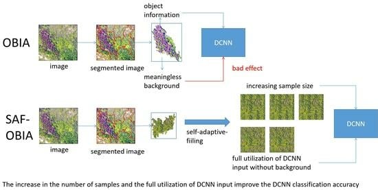
• We propose a self-adaptive-filling based OBIA to enhance the classification performance of a DCNN classifier using the OBIA technique (SAF-DCNN) for the remote sensing images of mountain vegetation.
• To demonstrate the advantages of SAF-based OBIA, we also compare the performance of using DCNN and random forest classifiers under SAF-based OBIA and traditional OBIA at two different data volumes.
• In addition, we compare the performance of OBIA-based methods with semantic segmentation methods on remote sensing images of mountain vegetation by comparing commonly used methods for the semantic segmentation of remote sensing images.

2. Materials and Methods

2.1. Study Area

Huaguo Mountain is located in the eastern suburb of Lianyungang, with longitude 119°13${}^{\prime }$–119°29${}^{\prime }$ east and latitude 34°34${}^{\prime }$–34°46${}^{\prime }$ north. The area is a transition zone between the warm temperate climate and the northern subtropical climate, characterized by a typical monsoon climate. The topography of the mountain slopes gently on the southeast side and becomes steeper on the northwest side. The region is characterized by an average elevation of approximately 300 m above sea level, a mean annual temperature of 14.1 °C, and an average annual rainfall of 943.3 mm.

Due to the influence of the oceanic climate, it creates ideal conditions for plant growth, including heat, light, humidity, and soil composition. These ideal conditions have contributed to the rich biodiversity of Huaguo Mountain, creating a natural wonder of rich vegetation and a wide variety of plants. The vegetation distribution of Huaguo Mountain is in a north–south transition; the larger forest areas are generally located on the gentle southern side, and the main vegetation species include Quercus acutissima, pine forests, and mixed coniferous and broad forests.

As depicted in Figure 1, we selected a segment of Huaguo Mountain as our study area, which, located at the south of the mountain range, tends to have gentle topographical features. Influenced by topography, there is a wide variety of vegetation, including Castanea mollissima, Quercus acutissima, Cunninghamia lanceolate, Pinus thunbergii, Pinus taeda, Phyllostachys Spectabilis, and Camellia sinensis. Remote sensing images of vegetation were classified using this study area to accurately represent the remote sensing image classification of vegetation types in mountainous areas.

2.2. Data

2.2.1. Data and Preprocessing

The data used in this study were provided by the Lianyungang Bureau of Natural Resources and Planning and were acquired using an unmanned aerial vehicle during spring 2018. The image includes three bands of RGB with a spatial resolution of 0.2 m. The quality of the image is fine and it was produced according to GDPJ 05-2013 [36] on the gentle south slope mountain. Therefore, the differences of the spectral and spatial characteristics of each vegetation type used for classification are mainly caused by vegetation spectral characteristics, composition, and structure. It has been orthorectified with GPS control points and DEM, and at last projected to the Chinese Geodetic Coordinate System 2000 (CGCS 2000).

2.2.2. Sample Data for Training and Verification

The sample data for training and verification in this study came from an existing forestry map, an in situ survey, and unmanned aerial vehicle (UAV) investigation. On the existing forestry map, while vegetation type information was displayed, we could only delineate sample data in some regions where one type of vegetation owned a large area and concentrated location, as shown in Figure 2. Nevertheless, in most cases, the limits of various vegetation types could not maintain good correspondence with 0.2 m spatial resolution aerial images when vegetation structure was fractal, for it was plotted based on a lower spatial resolution image. For example, as shown in Figure 3, the vegetation type had been plotted as Castanea mollissima on the forestry map; however, on the aerial image used in our study, two vegetation types, incuding Castanea mollissima and Quercus acutissima, could be represented. Therefore, for application to other study regions, field surveying is necessary to obtain sample data.

An in situ survey was carried out based on the aerial image, and was conducted by the Lianyungang Forestry Station technicians who were more familiar with the vegetation structure and its location in the study area. For the 0.2 m spatial resolution image, when the regions consist of only one vegetation type, it will tend to show relatively uniform spatial and spectral characteristics, which makes it very easy to discriminate any type of vegetation from surrounding vegetation, as shown in Figure 4. Accordingly, during the in situ survey process, when the vegetation types were identified in any accessible place, the sample data could be plotted. Using this method, for all the accessible regions, the sample data could be acquired via a combination of in situ survey and visual plotting.

An unmanned aerial vehicle (UAV) was deployed as a complementary technique when the chosen sample data were located in poor-accessibility regions because vegetation type classification requires high spatial resolution. Compared to other remote sensing equipment, UAV imagery offers centimeter-level resolution, enabling the correct determination of vegetation type data with the help of forestry technicians and experts. Shown in

Table 1. Pictures taken by UAV.

Vegetation Type	Picture Taken by UAV	Vegetation Type	Picture Taken by UAV
Phyllostachys Spectabilis		Quercus acutissima
Cunninghamia lanceolate		Pinus thunbergii

, these pictures were taken by a UAV at a height of approximately 60 m. Other vegetation types are either located at favorable accessibility regions, for example, Castanea mollissima, or have obvious image characteristics, for example, Pinus thunbergii and Camellia sinensis. Therefore, there are no sample data acquired from a UAV picture.

Figure 5 illustrates the final sample data obtained using the above three approaches, which were used as the training and verifying samples for this paper. This research ultimately subdivides the vegetation into ten categories, including Castanea mollissima, Quercus acutissima, Pinus thunbergii, and Cunninghamia lanceolate, among others. These specific classifications are shown in

Table 2. Mountain vegetation classification types.

Vegetation Type	Image	Description
Castanea mollissima		This is a tree with edible fruits. The leaves of the tree are characterized by their broad shape and haphazard arrangement. They exhibit vibrant hues and distinct spectral features.
Quercus acutissima		In the study area, Quercus acutissima is widely distributed in the mountain forests due to its remarkable adaptability. Quercus acutissima has smaller leaves than C. mollissima quercus, with dense, naturally occurring branches. Quercus acutissima has an inconspicuous crown, giving a distinctly “broken” silhouette.
Pinus thunbergii		This tree has a small canopy, little shading, low numbers, and random distribution in this study area. It appears black on the image, rarely pure forest, and is often mixed with green shrubs.
Cunninghamia lanceolate		This is similar in image to the textural features of the pine but the color differs from those of the P.thunbergii, which is a familiar brown color. It is more dense and slightly taller than the P.thunbergii in the study area.
Pinus taeda		The color of this vegetation on the image is similar to that of Cunninghamia lanceolate, but the textural features are different and the canopy is more pronounced than in Cunninghamia lanceolate.
Camellia sinensis		Artificially reclaimed Camellia sinensis with neatly shaped and distinctive features.
Phyllostachys Spectabilis		This vegetation looks smoother and more finely textured on the image, with distinctive features, but it is sometimes intermixed with trees whose canopies can partially obscure it.
Broadleaf Forest		A mixture of different species of broadleaf woods.
Shrub and Grass		This one appears to have no visible canopy on the image, and sometimes contains bare rocks or some other trees.
Mixed Broadleaf–Conifer Forest		Contains broadleaf and coniferous forests, mixed together.

.

2.3. Study Methods

2.3.1. Traditional Based OBIA

The typical workflow of conventional object-based image classification, commonly applied to high-resolution imagery, can be outlined in these primary steps: (1) The image is segmented using a pre-determined set of parameters (e.g., segmentation ratio and shape weights) to obtain a segmented image fragment, denoted as A. (2) The features of the object are extracted in the segmented image, such as the average spectral band values. That is, a series of functions $f1-fn$ (n is the number of features) are applied to an image A to obtain the feature vector a of that image, as shown in Equation (1).

$$a=[f_1\left(A\right),f_2\left(A\right),...f_n\left(A\right)].$$

(1)

(3) A part of the data from the array of feature vectors [$a_1,a_2,...,a_m$] (m is the number of pictures) is selected to train a classifier F, such as SVM or RF classifier. (4) The segmented image is classified using the trained classifier F. If the classifier is random forest, we will use OBIA-RF to represent this classifier. The process of applying DCNN directly within the conventional OBIA framework is referred to as OBIA-DCNN. Unlike OBIA-RF where the input is the features of the image, the input is an adaptively sized rectangular image patch (with the blanks filled with 0 values as the background) that contains the objects in their entirety. This process does not utilize all of the DCNN input pixels. Meanwhile, due to the complex and heterogeneous nature of mountainous terrain, it is difficult to obtain enough samples to stimulate the classification potential of DCNN. To address these two issues, we propose self-adaptive-filling based OBIA.

2.3.2. Self-Adaptive-Filling Based OBIA

In the SAF-based OBIA framework, the steps for classification based on traditional classifiers (e.g., SVM and RF) are as follows: (1) Segment the image using a set of predefined parameters, such as segmentation ratio and shape weights, to obtain a segmented image patch A. (2) Obtain multiple filled images [$A_1-A_I$] by filling the objects obtained from segmentation using the self-adaptive-filling method G proposed in this paper, as shown in Equation (2).

$$[A_1,A_2,...,A_I]=G\left(A\right).$$

(2)

(3) Extract the features of multiple filled images [$A_1-A_i$] for each object separately, using a series of functions $f_1-f_n$, such as the average band value and the feature ratio of the band value for the segmented image. The feature vector $a_i$ corresponding to the ith image generated by filling is shown in Equation (3).

$$a_{1\le i\le I}=[f_1\left(A_i\right),f_2\left(A_i\right),...f_n\left(A_i\right)].$$

(3)

(4) Train a classifier F, such as SVM or RF. (5) Use the trained classifier to classify the filled images of each object and then vote on the classification results to arrive at the final classification result. If the classifier is random forest, we will use SAF-RF to denote the classifier. For a particular original image patch A, its i filled images $A_1-A_I$ are predicted and the classification result $r_i$ for each filled image is obtained as shown in Equation (4).

$$r_{1\le i\le I}=F\left(a_i\right).$$

(4)

We obtain a set of classification results for the filled images $R=\{r_1,r_2,....,r_i\}$. The classification result r which occurs most times in the set R is used as the classification result of the original image patch A.

Similarly, if DCNN is used as a classifier for SAF-based OBIA, this classification method is referred to as SAF-DCNN. The steps for SAF-DCNN classification are similar to those mentioned above for SAF-based OBIA in traditional classification methods such as SAF-RF. The difference is that SAF-DCNN does not require the manual feature extraction process mentioned in step (3) above. The filled images are directly used to train the classifier F. Contrary to the conventional usage of DCNN in the traditional OBIA framework, we propose filling in the blank areas of the adaptive image patches—using the pixel blocks contained in the object itself—in order to eliminate the effect of other values contained in the adaptive image patches not of this object (meaningless background values or spectral values of the object’s surroundings) on the classification accuracy of the DCNN. In addition to this, the SAF-based OBIA expands the training set by using different blocks of pixels from the object itself for filling to obtain different image patches to input to the DCNN to enhance its performance. The detailed process of SAF-based OBIA classification is illustrated in Figure 6.

2.3.3. Filled Image Generation for SAF-Based OBIA

The purpose of this section is to illustrate how to generate filled images on a segmented object corresponding to that object to support SAF-based OBIA classification. We believe that the original information about the object should be left unaltered when using the object’s own pixels to fill in blank areas to generate rectangular, adaptive image patches. In addition, the filling kernels should preserve as much of the original spatial and spectral information as possible in order to make the filled image more similar to natural vegetation growth. Specific filled image generation is divided into three steps as follows: Firstly, cut the segmented image patches collected by OBIA to obtain image patches. Secondly, cut multiple filling kernels from each image patch to obtain multiple self-adaptive-filling kernels. Thirdly, fill each filling kernel into the original image patch to obtain the enhancement sample. The specific process is shown in Algorithm 1 and Figure 7.

Algorithm 1: Self-adaptive-filling Algorithm

Data: An image A of size $a\times b\times 3$ Result: An array $P[n,a,b]$ of n images of size $a\times b\times 3$ 1  Declare an array $K[n,c,c]$ to store the filling kernels, where c is the size of the sliding window ($c<b$ and $c<a$); 2  Initialize the sliding window size to $c\times c$; 3  Slide the window over the entire source image, ensuring that each pixel within the window is non-empty. Store the window in the filling kernels array K; 4  Slide the window by c pixels; 5  If the end of the image is reached, decrease the value of c; 6  Repeat steps 3–5 until n filling kernels are obtained; 7  Declare an output array $P[n,a,b]$; 8  Iterate over the filling kernels array K and obtain a filling kernel $K\left[i\right]$ (where $i=0$); 9  Find an empty pixel $A[x,y]$ in image A; 10  For each j and k in the range $(0,c)$:; 11     If $A[x+j,y+k]$ is not null:; 12        Set $A[x+j,y+k]$ to $K\left[i\right](0+j,0+k)$; 13  Repeat steps 9–12 until the entire image A is traversed. Set $P\left[i\right]$ to A; 14  Increment i by 1 and repeat steps 8–13 until all filling kernels in K are used; 15  Output the array of filled images P.

2.3.4. RF and DCNN Using SAF-Based OBIA for Experiments

For the experiments on the SAF-based OBIA method proposed in this paper on traditional classification methods, we chose a representative method, RF. Representative features including spectral features, texture features, and spectral indices were also selected. The details are shown in Table 3.

Table 3. Feature definitions and formulas.

Feature Category	Feature Name	Calculation Formula	Description
Spectral characteristics	Mean	$$\begin{array}{ccc}\hfill \hfill & \hfill {\mathrm{c}}_{\mathrm{k}}^{-}\left(o\right)\hfill & \hfill =\frac{1}{n}\sum _{(x,y)\in P_o}{c}_k(x,y)\hfill \end{array}$$ (5)	Grayscale values of all image elements in the kth band
	Standard Deviation	$$\begin{array}{ccc}\hfill \hfill & \hfill {\sigma }_k\left(o\right)\hfill & \hfill =\sqrt{\left(\sum _{(x,y)\in P_o}{c}_k^2(x,y)-\frac{1}{n}\left(\sum _{(x,y)\in P_o}{c}_k{(x,y)}^2\right)\right)\times \frac{1}{n}}\hfill \end{array}$$ (6)	Standard deviation of grayscale values of all image elements in the kth band
	Ratio	$$\mathrm{Ratio}=\frac{\overline{{\mathrm{c}}_{\mathrm{k}}}\left(o\right)}{{\sum }_{k=1}^K\overline{{\mathrm{c}}_{\mathrm{k}}}\left(o\right)}$$ (7)	The ratio of the mean grayscale value of the image in the kth band to the overall brightness of the object
Texture characteristics	Entropy	$$\sum _{i,j=0}^{N-1}{P}_{i,j}\left(-ln{P}_{i,j}\right)$$ (8)	Reflects the amount of information in the image object
	Homogeneity	$$\sum _{i,j=0}^{N-1}\frac{P_{i,j}}{1+{(i-j)}^2}$$ (9)	Reflects the intrinsic variability of the image object and the smaller the variance the larger the value
	Contrast	$$\sum _{i,j=0}^{N-1}{P}_{i,j}{(i-j)}^2$$ (10)	Reflects the degree of change in image objects and highlights anomalies
	Correlation	$$\sum _{i,j=0}^{N-1}\frac{P_{i,j}\left(i-{\mu }_i\right)\left(j-{\mu }_j\right)}{{\sigma }_i^2{\sigma }_j^2}$$ (11)	Reflects the degree of linear correlation of grayscale within the image object
	Angle Second Moment	$$\sum _{i,j=0}^{N-1}{P}_{i,j}^2$$ (12)	Reflects the uniformity of grayscale distribution within the image object
	Mean	$${\mu }_{i,j}=\frac{{\sum }_{i,j=0}^{N-1}{P}_{i,j}}{N^2}$$ (13)	Reflects the average grayscale within the image object
	Standard Deviation	$${\sigma }_{i,j}=\sqrt{\sum _{i,j=0}^{N-1}\left(P_{i,j}-{\mu }_{i,j}\right)}$$ (14)	Reflects the magnitude of grayscale changes within the image object
	Dissimilarity	$$\sum _{i,j=0}^{N-1}{P}_{i,j}|i-j|$$ (15)	Reflects the degree of grayscale detail variation within the image object
Vegetation Index	EXG	$$2\ast G-R-B$$ (16)	Over Green Index
	EXR	$$1.4\ast R-G$$ (17)	Super Red Index
	EXGR	$$EXG-EXR$$ (18)	Super Green Super Red Differential Index
	NGBD I	$$(G-B)/(G+B)$$ (19)	Normalized Green and Blue Disparity Index
	RGBV I	$$(G-B\ast R)/(G+B\ast R)$$ (20)	Red, Green, and Blue Vegetation Index
	NGRD I	$$(G-R)/(G+R)$$ (21)	Normalized Red–Green Variance Index

P_o is the set of image elements in object o; n is the number of image elements in p_o; c_k(x, y) is the gray value of the image element (x, y) in the k-band; $\overline{c_{\mathrm{k}}}\left(o\right)$ is the average value of all pixels in the k-band of the image; ${\sigma }_k\left(o\right)$ denotes the standard deviation of o in band k-band; K is the total number of bands involved in the operation; N stands for the number of gray levels; P_i,j represents the values of the elements in row i, column j of the grayscale covariance matrix; ${\mu }_{i,j}$ is the texture mean; ${\sigma }_{i,j}$ is the texture standard deviation; R is the red band spectral value; G is the green band spectral value; B is the blue band spectral value.

Table 3. Feature definitions and formulas.

Feature Category	Feature Name	Calculation Formula	Description
Spectral characteristics	Mean	$$\begin{array}{ccc}\hfill \hfill & \hfill {\mathrm{c}}_{\mathrm{k}}^{-}\left(o\right)\hfill & \hfill =\frac{1}{n}\sum _{(x,y)\in P_o}{c}_k(x,y)\hfill \end{array}$$ (5)	Grayscale values of all image elements in the kth band
	Standard Deviation	$$\begin{array}{ccc}\hfill \hfill & \hfill {\sigma }_k\left(o\right)\hfill & \hfill =\sqrt{\left(\sum _{(x,y)\in P_o}{c}_k^2(x,y)-\frac{1}{n}\left(\sum _{(x,y)\in P_o}{c}_k{(x,y)}^2\right)\right)\times \frac{1}{n}}\hfill \end{array}$$ (6)	Standard deviation of grayscale values of all image elements in the kth band
	Ratio	$$\mathrm{Ratio}=\frac{\overline{{\mathrm{c}}_{\mathrm{k}}}\left(o\right)}{{\sum }_{k=1}^K\overline{{\mathrm{c}}_{\mathrm{k}}}\left(o\right)}$$ (7)	The ratio of the mean grayscale value of the image in the kth band to the overall brightness of the object
Texture characteristics	Entropy	$$\sum _{i,j=0}^{N-1}{P}_{i,j}\left(-ln{P}_{i,j}\right)$$ (8)	Reflects the amount of information in the image object
	Homogeneity	$$\sum _{i,j=0}^{N-1}\frac{P_{i,j}}{1+{(i-j)}^2}$$ (9)	Reflects the intrinsic variability of the image object and the smaller the variance the larger the value
	Contrast	$$\sum _{i,j=0}^{N-1}{P}_{i,j}{(i-j)}^2$$ (10)	Reflects the degree of change in image objects and highlights anomalies
	Correlation	$$\sum _{i,j=0}^{N-1}\frac{P_{i,j}\left(i-{\mu }_i\right)\left(j-{\mu }_j\right)}{{\sigma }_i^2{\sigma }_j^2}$$ (11)	Reflects the degree of linear correlation of grayscale within the image object
	Angle Second Moment	$$\sum _{i,j=0}^{N-1}{P}_{i,j}^2$$ (12)	Reflects the uniformity of grayscale distribution within the image object
	Mean	$${\mu }_{i,j}=\frac{{\sum }_{i,j=0}^{N-1}{P}_{i,j}}{N^2}$$ (13)	Reflects the average grayscale within the image object
	Standard Deviation	$${\sigma }_{i,j}=\sqrt{\sum _{i,j=0}^{N-1}\left(P_{i,j}-{\mu }_{i,j}\right)}$$ (14)	Reflects the magnitude of grayscale changes within the image object
	Dissimilarity	$$\sum _{i,j=0}^{N-1}{P}_{i,j}|i-j|$$ (15)	Reflects the degree of grayscale detail variation within the image object
Vegetation Index	EXG	$$2\ast G-R-B$$ (16)	Over Green Index
	EXR	$$1.4\ast R-G$$ (17)	Super Red Index
	EXGR	$$EXG-EXR$$ (18)	Super Green Super Red Differential Index
	NGBD I	$$(G-B)/(G+B)$$ (19)	Normalized Green and Blue Disparity Index
	RGBV I	$$(G-B\ast R)/(G+B\ast R)$$ (20)	Red, Green, and Blue Vegetation Index
	NGRD I	$$(G-R)/(G+R)$$ (21)	Normalized Red–Green Variance Index

P_o is the set of image elements in object o; n is the number of image elements in p_o; c_k(x, y) is the gray value of the image element (x, y) in the k-band; $\overline{c_{\mathrm{k}}}\left(o\right)$ is the average value of all pixels in the k-band of the image; ${\sigma }_k\left(o\right)$ denotes the standard deviation of o in band k-band; K is the total number of bands involved in the operation; N stands for the number of gray levels; P_i,j represents the values of the elements in row i, column j of the grayscale covariance matrix; ${\mu }_{i,j}$ is the texture mean; ${\sigma }_{i,j}$ is the texture standard deviation; R is the red band spectral value; G is the green band spectral value; B is the blue band spectral value.

The limitation of traditional classifiers is that features must be selected manually. Improper feature selection will reduce the classification accuracy. SAF-based OBIA using DCNN can effectively avoid the accuracy problem caused by improper manual feature selection. To begin with, SAF-based OBIA collects patches of segmented images. Subsequently, multiple filling kernels are cut from each image patch to obtain multiple filling kernels. Lastly, each filling kernel is filled into the original image patch to obtain the enhancement sample. Finally, all the enhanced samples are classified and then voted on to obtain the final classification results. In the experimental stage, we refer to the OSA-CNN proposed by Jie Wang [25] and use the DCNN classification module in OSA-CNN to conduct experiments.

2.3.5. RF and DCNN Using OBIA for Comparison

Object-Based Image Analysis (OBIA) is a significant tool for target detection in remote sensing imagery, as referenced in [37]. Therefore, in order to measure the effectiveness of SAF-based OBIA proposed in this paper, it was compared with random forest and DCNN based on traditional OBIA. The comparison was built on exactly the same training and testing sets. When using random forest, the same features were selected as in the SAF-based OBIA experiments, all shown in Table 3. The exact same network structure as in the SAF-based OBIA experiment was also used when employing DCNN as a classifier.

2.3.6. Semantic Segmentation: U-net, MACU-net, and SegNeXt for Comparison

Semantic segmentation has been widely used in many fields with better results. Among them, U-net [38] is a deep learning architecture for image segmentation. It was initially proposed for medical image segmentation and was later used in other fields, such as remote sensing, with good results. The network structure of U-net is a symmetric encoder and decoder with a hopping connection path in between. The encoder part consists of a series of convolutional layers and pooling layers for extracting image features and gradually reducing the spatial resolution. The decoder part consists of a series of convolutional layers and upsampling layers to gradually restore the feature map to its original size and generate segmentation results. We chose U-net for comparison because its accuracy in tree species recognition is similar to two other classical semantic segmentation methods, SegNet and FCDenseNet, but it is easier to train [39].

Proposed in 2015, U-net is widely used in remote sensing with good results. In order to increase the persuasiveness of the comparison experiments, we chose the MACU-net [40] method based on the improvement in U-net++. MACU-net is a network that was proposed by Rui Li in 2021. The network also enhances the feature representation and extraction capabilities of the standard convolutional layers with asymmetric convolutional blocks. The proponents of this method have experimentally demonstrated, on two remote sensing datasets captured by different satellite sensors, that the method (i.e., MACU-Net) outperforms benchmark methods such as U-Net, U-Net 3+, and U-Net with PPL.

SegNeXt [41] is a recently proposed semantic segmentation method. This approach uses convolutional attention to encode contextual information more effectively than the self-attention mechanism in transformers. SegNeXt substantially enhances the performance on well-recognized benchmarks compared to preceding cutting-edge methods, including ADE20K, Cityscapes, COCO-Stuff, Pascal VOC, Pascal Context, and iSAID. We chose this method comparison to make up for our shortcomings regarding the new method comparison.

2.3.7. Experiment Design

This section aims to delineate the experimental framework designed to accomplish the research objectives outlined in the introductory section. Firstly, once the original images were acquired, they were labeled via visual interpretation and field visits, and the original and labeled sample images were obtained by combining the results of previous forestry surveys. Then, the images were cropped into two groups of image patches according to the different requirements of OBIA and semantic segmentation. Using OBIA-based methods, we determined the optimal segmentation ratio and shape weights for image segmentation based on experiments and expert experience. All OBIA methods use the same segmentation ratio and shape weights. Each set of image patches was divided into two equal numbers of copies, one for the training set and one for the testing set. A quarter of the training set was then randomly selected from the training set as a small sample. Figure 8 summarizes the experiments performed using the SAF-based OBIA approaches, the traditional OBIA approaches, and the semantic segmentation approaches to compare the performance of each approach on two datasets with different data volumes.

3. Results

3.1. Overall Accuracy Evaluation

Overall Accuracy (OA) is a common metric for evaluating the performance of a classification model [42,43,44] and it is given by

$$OA=(TP+TN)/(TP+FP+TN+FN),$$

(22)

The Kappa coefficient is a statistical metric that is also commonly used for classification accuracy assessment [43,44,45] and it is calculated as follows:

$$\kappa =\frac{P_o-P_e}{1-P_e}$$

(23)

MIoU refers to mean intersection over union. It is a common measure of image segmentation accuracy and is used in computer vision tasks such as target detection and semantic segmentation.

$$\mathrm{mIoU}=\frac{1}{n_{\mathrm{cl}}}\sum _{i=1}^{n_{\mathrm{cl}}}\left(\frac{p_{ii}}{{\sum }_{j=1}^{t_i}{p}_{ij}+{\sum }_{j=1}^{t_i}{p}_{ji}-p_{ii}}\right)$$

(24)

$n_{\mathrm{cl}}$ represents the total number of classes. $p_{ij}$ is the count of pixels of class i predicted to belong to class j. $t_i$ is the total count of pixels belonging to class i. $p_{ii}$ is the count of pixels of class i that were correctly predicted.

The results of OA, Kappa, and mIoU coefficients for all experiments in this paper are shown in Figure 9.

3.2. Accuracy of Each Vegetation

The evaluation metrics known as User’s Accuracy (UA) and Producer’s Accuracy (PA) are frequently employed in fields such as remote sensing imagery and feature classification to assess the precision of classification outcomes.

UA is the number of samples correctly predicted out of the total number of samples predicted in the category from a prediction point of view.

PA is the number of correctly predicted samples from the perspective of the sample as a percentage of the total number of samples in the category.

These two metrics are commonly used to evaluate the performance of classification algorithms [43,46,47], and can help to determine the reliability of the classification results and the effectiveness of the classifier. The producer and user accuracies for each method and each vegetation are shown in

Table 4. Specific results of vegetation classification.

		Castanea mollissima	Quercus acutissima	Pinus thunbergii	Cunninghamia lanceolate	Pinus taeda	Camellia sinensis	Phyllostachys Spectabilis	Broadleaf Forest	Shrub and Grass	Mixed Broadleaf–Conifer Forest
SAF-RF-DR *	PA	0.177	0.565	0.547	0.520	0.546	0.800	1.000	0.354	0.647	0.467
	UA	0.214	0.718	0.265	0.520	0.300	0.348	0.125	0.193	0.734	0.525
SAF-DCNN-DR	PA	0.568	0.745	0.667	0.633	0.750	0.696	0.750	0.467	0.745	0.660
	UA	0.595	0.708	0.623	0.740	0.545	0.696	0.375	0.523	0.784	0.635
OBIA-RF-DR	PA	0.286	0.463	0.497	0.471	0.500	0.667	0.500	0.300	0.644	0.401
	UA	0.098	0.634	0.307	0.519	0.045	0.087	0.125	0.199	0.703	0.411
OBIA-DCNN-DR	PA	0.632	0.814	0.628	0.652	0.069	0.875	1.000	0.473	0.724	0.719
	UA	0.571	0.759	0.689	0.779	0.273	0.913	0.500	0.464	0.784	0.462
U-net-DR	PA	0.403	0.596	0.460	0.536	0.342	0.611	0.451	0.255	0.603	0.488
	UA	0.372	0.684	0.324	0.449	0.603	0.453	0.070	0.228	0.674	0.456
MACU-net-DR	PA	0.604	0.771	0.679	0.587	0.503	0.712	0.000	0.511	0.725	0.611
	UA	0.502	0.764	0.671	0.567	0.470	0.661	0.000	0.362	0.770	0.718
SAF-RF-DP *	PA	0.750	0.477	0.478	0.432	0.250	0.556	0.000	0.274	0.632	0.409
	UA	0.071	0.706	0.214	0.416	0.050	0.217	0.000	0.133	0.713	0.442
SAF-DCNN-DP	PA	0.575	0.659	0.656	0.592	0.563	1.000	0.000	0.453	0.660	0.542
	UA	0.548	0.704	0.483	0.623	0.409	0.652	0.000	0.351	0.796	0.522
OBIA-RF-DP	PA	0.000	0.432	0.450	0.421	0.000	0.000	0.000	0.234	0.577	0.292
	UA	0.000	0.597	0.249	0.312	0.000	0.000	0.000	0.166	0.680	0.324
OBIA-DCNN-DP	PA	0.190	0.670	0.571	0.613	0.800	1.000	0.000	0.364	0.635	0.526
	UA	0.095	0.699	0.420	0.597	0.182	0.522	0.000	0.318	0.826	0.482
U-net-DP	PA	0.014	0.261	0.149	0.060	0.010	0.031	0.010	0.076	0.277	0.105
	UA	0.009	0.113	0.124	0.252	0.066	0.078	0.006	0.080	0.284	0.032
MACU-net-DP	PA	0.426	0.679	0.542	0.624	0.312	0.000	0.000	0.486	0.694	0.495
	UA	0.431	0.676	0.578	0.554	0.219	0.000	0.000	0.352	0.704	0.657

* DR stands for data-rich representing a well-sampled experiment. * DP stands for data-poor, representing a poorly sampled experiment. The best results for these two different sample sizes are shown in bold.

.

3.3. Classification Results Map

In order to compare the performance of OBIA-based methods and semantic segmentation methods in the classification of vegetation types in mountainous areas, this paper chooses the MACU-net-DR method, which has the best effect of semantic segmentation, and the SAF-DCNN-DR method, which has the best effect based on OBIA. The results of classifying the whole study area using these two methods are shown in Figure 10.

4. Discussion

4.1. Performance of SAF-DCNN on Mountain Vegetation Classification

When the data volume is small, SAF-DCNN has obvious advantages in the remote sensing of mountain vegetation. As shown in Figure 9, the results of this method are 0.624 in OA, 0.529 in Kappa, and 0.386 in mIoU, which are the highest among all compared methods. When the amount of data is large, SAF-DCNN is 0.685 in OA, only 0.002 lower than MACU-net, which has the highest accuracy. Both SAF-DCNN and MACU-net achieved the highest kappa of 0.495. For the kappa metric, SAF-DCNN’s 0.610 is nearly 0.003 lower than the highest MACU-net’s 0.613. However, due to the pretzel phenomenon present in the results of semantic segmentation, the results of SAF-DCNN are still more visually appealing than MACU-net. For the evaluation metric of mIoU, SAF-DCNN was 0.472, only 0.006 lower than the highest OBIA-DCNN of 0.478. To further compare SAF-DCNN and OBIA-DCNN, we performed a ten-fold cross-validation and t-test, and the results are shown in

Table 5. The 10-fold cross-validation and t-test results.

Classifiers	SAF-DCNN	OBIA-DCNN
Fold #1	0.662	0.635
Fold #2	0.651	0.621
Fold #3	0.649	0.652
Fold #4	0.729	0.688
Fold #5	0.694	0.658
Fold #6	0.698	0.653
Fold #7	0.686	0.667
Fold #8	0.675	0.630
Fold #9	0.674	0.649
Fold #10	0.673	0.665
Mean	0.679	0.651
Pairwise t-test	t:5.549 p:0.00357 1

¹ p < 0.01.

. The results showed statistically significant differences between these two methods.

In order to check the robustness of SAF-DCNN, we performed a validation for two other regions of Huaguo Mountain (as shown in Figure 11). The results are shown in

Table 6. The OA, Kappa, and mIoU in Region A and Region B.

Region	OA	Kappa	mIoU
Region A	0.694	0.573	0.403
Region B	0.624	0.461	0.426

.

Region A is similar in size, has a similar sample size, and has similar overall evaluation metrics to the study area. Region B is smaller than the study area, with a smaller sample size and slightly lower evaluation indicators than the study area.

4.2. Performance of SAF-Based OBIA

From Figure 9, it can be seen that SAF-DCNN proposed in this paper has some improvement over the OBIA-DCNN in both OA and Kappa evaluation metrics. In the case of a larger data volume, the improvement in OA is smaller, from 0.673 to 0.685, while in the case of a smaller data volume, the improvement is more obvious, from 0.597 to 0.624. Similarly, Kappa improves less with larger amounts of data, from 0.488 to 0.495, and more significantly with smaller amounts of data, from 0.39 to 0.422. This may be due to the fact that our proposed SAF-based OBIA can increase the number of samples and stimulate the potential of DCNN without relying on additional data. However, there are some types of vegetation with reduced accuracy, which may be due to the padding method blurring the boundary of vegetation in image segmentation.

Meanwhile, SAF-RF, which combines the SAF-based OBIA framework proposed in this paper with RF, also performs better relative to the traditional OBIA-RF. As shown in Figure 9 regarding the evaluation metric of OA, there is an improvement of five percentage points at high data volume and six percentage points at low data volume. For Kappa, the evaluation metric, there is an improvement of about five percentage points for both different data volumes. The analysis in this paper suggests that the following two reasons may have boosted RF performance. The first is that SAF’s expansion of the sample also helps RF. The second is that there is a change in the image features after self-adaptive-filling processing, as shown in Figure 12. It may be that this change is more favorable than RF for classification.

4.3. Comparison of OBIA and Semantic Segmentation in Mountain Vegetation Classification

In this research, four OBIA-based methods and two semantic-segmentation-based methods are selected for comparison. The four OBIA-based methods are the traditional OBIA based on manually selected features and OBIA-RF with random forest, OBIA-DCNN combined with DCNN classification, the improved SAF-DCNN based on OBIA-DCNN, and improved SAF-RF based on OBIA-RF proposed in this paper. The two semantic segmentation methods are the classical U-net and the improved MACU-net based on the U-net proposed in 2021. From the experimental results in Figure 9, it is seen that the accuracy assessment of the newer classifiers in OBIA using DCNN and the newer methods in semantic segmentation using MACU-net are similar at large data volumes. However, as can be seen in Figure 13, the OBIA-based approach effectively mitigates the pretzel phenomenon produced by the semantic segmentation approach. In the case of small data volume where the amount of data is not sufficient, the OBIA-based method, SAF-DCNN, has a slight advantage in accuracy (two percentage points higher). This suggests that the OBIA-based method can better minimize the negative impact of insufficient sample size relative to the semantic-segmentation-based method.

5. Conclusions

This study represents an early application of DCNN-based OBIA for vegetation classification in mountainous areas. In this way, we have achieved better results than traditional OBIA based on manually selected features. We also propose an improvement called SAF-based OBIA (self-adaptive-filling based OBIA) because it not only integrates OBIA and DCNN, but it also utilizes the pixels contained in the object itself to fill the null-valued region around the object. Therefore, each pixel of the image input to the DCNN classifier is meaningful. It also increases the number of samples fed into the DCNN classifier (in this experiment it is five times the original sample size). SAF-based OBIA triggers the capability of the DCNN classifier more efficiently via training on the augmented dataset. For this reason, the accuracy is improved in the case of the same DCNN classifiers, and this improvement can be large when the original training set is small. It effectively alleviates the problem of obtaining sufficient samples due to intricate vegetation in mountainous areas. Meanwhile, the improved method of SAF-based OBIA proposed in this paper also improves classification accuracy when acting on traditional classification methods such as random forest.

In addition, this study compares the performances of the OBIA-based approach and the semantic-segmentation-based approach on mountain vegetation classification. In terms of large data volume, the accuracy evaluation of the two method types is similar. However, OBIA-based methods do not produce the pretzel phenomenon that is common in semantic-segmentation-based methods. The accuracy of OBIA-based methods is higher than for semantic segmentation at a small data volume. Although the accuracy evaluation of the new methods in the two classes of methods is similar in terms of the amount of large data, since the OBIA-based method does not produce the pretzel phenomenon of the semantic-segmentation-based method, this paper concludes that the OBIA-based method is superior to the semantic-segmentation-based method. This may be because DCNN, especially DCNN in semantic segmentation methods, requires a large amount of data. However, the SAF-based OBIA proposed in this paper can enhance the dataset to improve the performance of the DCNN classifier. In conclusion, an OBIA-based approach is superior to a semantic-segmentation-based approach.

We believe that our methodology has implications for forestry and conservation, and that it provides a new option for classifying and identifying forest types and species. This will help foresters to better understand and manage forest resources, protect endangered species, and maintain biodiversity. Additionally, utilizing our method for more accurate vegetation classification can improve the efficiency of forest conservation and management.

Last, we believe it is necessary to test the effects of the segmentation parameter pairs, DCNN output sample size, and filling kernel size in Algorithm 1 on SAF-based OBIA classification accuracy. It is also interesting to explore why SAF-based OBIA can increase the classification accuracy of random forests. However, the problem with SAF is that it produces extra samples, which can be difficult due to storage space and training time. We hope to reduce this extra resource consumption in our subsequent work.

References

1. Pettorelli, N.; Schulte to Bühne, H.; Tulloch, A.; Dubois, G.; Macinnis-Ng, C.; Queirós, A.M.; Keith, D.A.; Wegmann, M.; Schrodt, F.; Stellmes, M.; et al. Satellite remote sensing of ecosystem functions: Opportunities, challenges and way forward. Remote Sens. Ecol. Conserv. 2018, 4, 71–93. [Google Scholar] [CrossRef]
2. Fassnacht, F.E.; Latifi, H.; Stereńczak, K.; Modzelewska, A.; Lefsky, M.; Waser, L.T.; Straub, C.; Ghosh, A. Review of studies on tree species classification from remotely sensed data. Remote Sens. Environ. 2016, 186, 64–87. [Google Scholar] [CrossRef]
3. White, J.C.; Coops, N.C.; Wulder, M.A.; Vastaranta, M.; Hilker, T.; Tompalski, P. Remote sensing technologies for enhancing forest inventories: A review. Can. J. Remote Sens. 2016, 42, 619–641. [Google Scholar] [CrossRef]
4. Jurado, J.M.; López, A.; Pádua, L.; Sousa, J.J. Remote sensing image fusion on 3D scenarios: A review of applications for agriculture and forestry. Int. J. Appl. Earth Obs. Geoinf. 2022, 112, 102856. [Google Scholar] [CrossRef]
5. Atzberger, C.; Darvishzadeh, R.; Schlerf, M.; Le Maire, G. Suitability and adaptation of PROSAIL radiative transfer model for hyperspectral grassland studies. Remote Sens. Lett. 2013, 4, 55–64. [Google Scholar] [CrossRef]
6. Mulla, D.J. Twenty five years of remote sensing in precision agriculture: Key advances and remaining knowledge gaps. Biosyst. Eng. 2013, 114, 358–371. [Google Scholar] [CrossRef]
7. Becker, A.; Russo, S.; Puliti, S.; Lang, N.; Schindler, K.; Wegner, J.D. Country-wide retrieval of forest structure from optical and SAR satellite imagery with deep ensembles. ISPRS J. Photogramm. Remote Sens. 2023, 195, 269–286. [Google Scholar] [CrossRef]
8. Jamison, E.A.K.; D’Amato, A.W.; Dodds, K.J. Describing a landscape mosaic: Forest structure and composition across community types and management regimes in inland northeastern pitch pine barrens. For. Ecol. Manag. 2023, 536, 120859. [Google Scholar] [CrossRef]
9. Rybansky, M. Determination of Forest Structure from Remote Sensing Data for Modeling the Navigation of Rescue Vehicles. Appl. Sci. 2022, 12, 3939. [Google Scholar] [CrossRef]
10. Ranjan, R. Linking green bond yields to the species composition of forests for improving forest quality and sustainability. J. Clean. Prod. 2022, 379, 134708. [Google Scholar] [CrossRef]
11. Edelmann, P.; Ambarlı, D.; Gossner, M.M.; Schall, P.; Ammer, C.; Wende, B.; Schulze, E.D.; Weisser, W.W.; Seibold, S. Forest management affects saproxylic beetles through tree species composition and canopy cover. For. Ecol. Manag. 2022, 524, 120532. [Google Scholar] [CrossRef]
12. Nasiri, V.; Beloiu, M.; Darvishsefat, A.A.; Griess, V.C.; Maftei, C.; Waser, L.T. Mapping tree species composition in a Caspian temperate mixed forest based on spectral-temporal metrics and machine learning. Int. J. Appl. Earth Obs. Geoinf. 2023, 116, 103154. [Google Scholar] [CrossRef]
13. Cavender-Bares, J.; Schneider, F.D.; Santos, M.J.; Armstrong, A.; Carnaval, A.; Dahlin, K.M.; Fatoyinbo, L.; Hurtt, G.C.; Schimel, D.; Townsend, P.A.; et al. Integrating remote sensing with ecology and evolution to advance biodiversity conservation. Nat. Ecol. Evol. 2022, 6, 506–519. [Google Scholar] [CrossRef] [PubMed]
14. Chen, X.; Avtar, R.; Umarhadi, D.A.; Louw, A.S.; Shrivastava, S.; Yunus, A.P.; Khedher, K.M.; Takemi, T.; Shibata, H. Post-typhoon forest damage estimation using multiple vegetation indices and machine learning models. Weather Clim. Extrem. 2022, 38, 100494. [Google Scholar] [CrossRef]
15. Peereman, J.; Hogan, J.A.; Lin, T.C. Intraseasonal interactive effects of successive typhoons characterize canopy damage of forests in Taiwan: A remote sensing-based assessment. For. Ecol. Manag. 2022, 521, 120430. [Google Scholar] [CrossRef]
16. Pawlik, Ł.; Harrison, S.P. Modelling and prediction of wind damage in forest ecosystems of the Sudety Mountains, SW Poland. Sci. Total Environ. 2022, 815, 151972. [Google Scholar] [CrossRef]
17. Marlier, M.E.; Resetar, S.A.; Lachman, B.E.; Anania, K.; Adams, K. Remote sensing for natural disaster recovery: Lessons learned from Hurricanes Irma and Maria in Puerto Rico. Environ. Sci. Policy 2022, 132, 153–159. [Google Scholar] [CrossRef]
18. Sun, Y.; Huang, J.; Ao, Z.; Lao, D.; Xin, Q. Deep learning approaches for the mapping of tree species diversity in a tropical wetland using airborne LiDAR and high-spatial-resolution remote sensing images. Forests 2019, 10, 1047. [Google Scholar] [CrossRef]
19. Sothe, C.; De Almeida, C.; Schimalski, M.B.; Liesenberg, V.; La Rosa, L.; Castro, J.; Feitosa, R.Q. A comparison of machine and deep-learning algorithms applied to multisource data for a subtropical forest area classification. Int. J. Remote Sens. 2020, 41, 1943–1969. [Google Scholar] [CrossRef]
20. Wagner, F.H.; Sanchez, A.; Tarabalka, Y.; Lotte, R.G.; Ferreira, M.P.; Aidar, M.P.; Gloor, E.; Phillips, O.L.; Aragao, L.E. Using the U-net convolutional network to map forest types and disturbance in the Atlantic rainforest with very high resolution images. Remote Sens. Ecol. Conserv. 2019, 5, 360–375. [Google Scholar] [CrossRef]
21. Kattenborn, T.; Eichel, J.; Fassnacht, F.E. Convolutional Neural Networks enable efficient, accurate and fine-grained segmentation of plant species and communities from high-resolution UAV imagery. Sci. Rep. 2019, 9, 17656. [Google Scholar] [CrossRef] [PubMed]
22. Fricker, G.A.; Ventura, J.D.; Wolf, J.A.; North, M.P.; Davis, F.W.; Franklin, J. A convolutional neural network classifier identifies tree species in mixed-conifer forest from hyperspectral imagery. Remote Sens. 2019, 11, 2326. [Google Scholar] [CrossRef]
23. Jiang, S.; Yao, W.; Heurich, M. Dead wood detection based on semantic segmentation of VHR aerial CIR imagery using optimized FCN-Densenet. Int. Arch. Photogramm. Remote Sens. Spat. Inf. Sci. 2019, 42, 127–133. [Google Scholar] [CrossRef]
24. Ye, W.; Lao, J.; Liu, Y.; Chang, C.C.; Zhang, Z.; Li, H.; Zhou, H. Pine pest detection using remote sensing satellite images combined with a multi-scale attention-UNet model. Ecol. Inform. 2022, 72, 101906. [Google Scholar] [CrossRef]
25. Wang, J.; Zheng, Y.; Wang, M.; Shen, Q.; Huang, J. Object-scale adaptive convolutional neural networks for high-spatial resolution remote sensing image classification. IEEE J. Sel. Top. Appl. Earth Obs. Remote Sens. 2020, 14, 283–299. [Google Scholar] [CrossRef]
26. Shui, W.; Li, H.; Zhang, Y.; Jiang, C.; Zhu, S.; Wang, Q.; Liu, Y.; Zong, S.; Huang, Y.; Ma, M. Is an Unmanned Aerial Vehicle (UAV) Suitable for Extracting the Stand Parameters of Inaccessible Underground Forests of Karst Tiankeng? Remote Sens. 2022, 14, 4128. [Google Scholar] [CrossRef]
27. Zhu, Y.; Zeng, Y.; Zhang, M. Extract of land use/cover information based on HJ satellites data and object-oriented classification. Trans. Chin. Soc. Agric. Eng. 2017, 33, 258–265. [Google Scholar]
28. Chen, H.; Yin, D.; Chen, J.; Chen, Y. Automatic Spectral Representation With Improved Stacked Spectral Feature Space Patch (ISSFSP) for CNN-Based Hyperspectral Image Classification. IEEE Trans. Geosci. Remote Sens. 2022, 60, 4709014. [Google Scholar] [CrossRef]
29. Sidike, P.; Sagan, V.; Maimaitijiang, M.; Maimaitiyiming, M.; Shakoor, N.; Burken, J.; Mockler, T.; Fritschi, F.B. dPEN: Deep Progressively Expanded Network for mapping heterogeneous agricultural landscape using WorldView-3 satellite imagery. Remote Sens. Environ. 2019, 221, 756–772. [Google Scholar] [CrossRef]
30. Zhang, C.; Pan, X.; Li, H.; Gardiner, A.; Sargent, I.; Hare, J.; Atkinson, P.M. A hybrid MLP-CNN classifier for very fine resolution remotely sensed image classification. ISPRS J. Photogramm. Remote Sens. 2018, 140, 133–144. [Google Scholar] [CrossRef]
31. Liu, T.; Abd-Elrahman, A.; Morton, J.; Wilhelm, V.L. Comparing fully convolutional networks, random forest, support vector machine, and patch-based deep convolutional neural networks for object-based wetland mapping using images from small unmanned aircraft system. GIScience Remote Sens. 2018, 55, 243–264. [Google Scholar] [CrossRef]
32. Ma, L.; Li, M.; Ma, X.; Cheng, L.; Du, P.; Liu, Y. A review of supervised object-based land-cover image classification. ISPRS J. Photogramm. Remote Sens. 2017, 130, 277–293. [Google Scholar] [CrossRef]
33. dos Santos Ferreira, A.; Freitas, D.M.; da Silva, G.G.; Pistori, H.; Folhes, M.T. Weed detection in soybean crops using ConvNets. Comput. Electron. Agric. 2017, 143, 314–324. [Google Scholar] [CrossRef]
34. Hartling, S.; Sagan, V.; Sidike, P.; Maimaitijiang, M.; Carron, J. Urban tree species classification using a WorldView-2/3 and LiDAR data fusion approach and deep learning. Sensors 2019, 19, 1284. [Google Scholar] [CrossRef] [PubMed]
35. Liu, T.; Abd-Elrahman, A. Deep convolutional neural network training enrichment using multi-view object-based analysis of Unmanned Aerial systems imagery for wetlands classification. ISPRS J. Photogramm. Remote Sens. 2018, 139, 154–170. [Google Scholar] [CrossRef]
36. Office of the Leading Group of the First National Geographic Census of the State Council. Technical Regulations for the Production of Digital Orthophotos; Technical Report 05-2013; Office of the Leading Group of the First National Geographic Census of the State Council: Beijing, China, 2013. [Google Scholar]
37. Cheng, G.; Han, J. A survey on object detection in optical remote sensing images. ISPRS J. Photogramm. Remote Sens. 2016, 117, 11–28. [Google Scholar] [CrossRef]
38. Ronneberger, O.; Fischer, P.; Brox, T. U-net: Convolutional networks for biomedical image segmentation. In Medical Image Computing and Computer-Assisted Intervention—MICCAI 2015, Proceedings of the 18th International Conference, Munich, Germany, 5–9 October 2015; Proceedings, Part III 18; Springer: Cham, Switzerland, 2015; pp. 234–241. [Google Scholar]
39. Lobo Torres, D.; Queiroz Feitosa, R.; Nigri Happ, P.; Elena Cué La Rosa, L.; Marcato Junior, J.; Martins, J.; Olã Bressan, P.; Gonçalves, W.N.; Liesenberg, V. Applying fully convolutional architectures for semantic segmentation of a single tree species in urban environment on high resolution UAV optical imagery. Sensors 2020, 20, 563. [Google Scholar] [CrossRef]
40. Li, R.; Duan, C.; Zheng, S. Macu-net semantic segmentation from high-resolution remote sensing images. arXiv 2020, arXiv:2007.13083. [Google Scholar]
41. Guo, M.H.; Lu, C.Z.; Hou, Q.; Liu, Z.; Cheng, M.M.; Hu, S.m. SegNeXt: Rethinking Convolutional Attention Design for Semantic Segmentation. In Advances in Neural Information Processing Systems; Koyejo, S., Mohamed, S., Agarwal, A., Belgrave, D., Cho, K., Oh, A., Eds.; Curran Associates, Inc.: Red Hook, NY, USA, 2022; Volume 35, pp. 1140–1156. [Google Scholar]
42. Fraiwan, M.; Faouri, E. On the automatic detection and classification of skin cancer using deep transfer learning. Sensors 2022, 22, 4963. [Google Scholar] [CrossRef]
43. Fei, H.; Fan, Z.; Wang, C.; Zhang, N.; Wang, T.; Chen, R.; Bai, T. Cotton classification method at the county scale based on multi-features and random forest feature selection algorithm and classifier. Remote Sens. 2022, 14, 829. [Google Scholar] [CrossRef]
44. Zhao, Y.; Zhu, W.; Wei, P.; Fang, P.; Zhang, X.; Yan, N.; Liu, W.; Zhao, H.; Wu, Q. Classification of Zambian grasslands using random forest feature importance selection during the optimal phenological period. Ecol. Indic. 2022, 135, 108529. [Google Scholar] [CrossRef]
45. Feizizadeh, B.; Darabi, S.; Blaschke, T.; Lakes, T. QADI as a new method and alternative to kappa for accuracy assessment of remote sensing-based image classification. Sensors 2022, 22, 4506. [Google Scholar] [CrossRef] [PubMed]
46. Neyns, R.; Canters, F. Mapping of urban vegetation with high-resolution remote sensing: A review. Remote Sens. 2022, 14, 1031. [Google Scholar] [CrossRef]
47. Faruque, M.J.; Vekerdy, Z.; Hasan, M.Y.; Islam, K.Z.; Young, B.; Ahmed, M.T.; Monir, M.U.; Shovon, S.M.; Kakon, J.F.; Kundu, P. Monitoring of land use and land cover changes by using remote sensing and GIS techniques at human-induced mangrove forests areas in Bangladesh. Remote Sens. Appl. Soc. Environ. 2022, 25, 100699. [Google Scholar] [CrossRef]
Figure 1. All proposed classifications were tested in an area of 1680 m × 1939 m, which is part of the Huaguoshan Forest, located in the southern part of Jiangsu Province, China, near the city of Lianyungang.
Remotesensing 16 00031 g001
Figure 2. Large area of Quercus acutissima with a concentrated location in the largest area wrapped by the red line.
Remotesensing 16 00031 g002
Figure 3. Region with fractal and complex structure including two kinds of tree species in the largest area wrapped by the red line.
Remotesensing 16 00031 g003
Figure 4. As shown by the purple lines wrapping each area on the map, the region consisting of only one vegetation type with relatively uniform spatial and spectral characteristics.
Remotesensing 16 00031 g004
Figure 5. The final sample data are shown in the figure.
Remotesensing 16 00031 g005
Figure 6. As shown in the figure, all the segmented image patches are segregated into train and test sets. Subsequently, the self-adaptive-filling procedure is performed on each set to obtain filled images for classifier training and prediction. The trained classifier is then used to predict multiple images generated from the same segmented object and finally vote for the final classification result. The classifier in the figure can use traditional classification methods such as SVM, RF, or DCNN.
Remotesensing 16 00031 g006
Figure 7. This figure illustrates the specific flow of the self-adaptive-filling algorithm. The red boxes are the selected filling kernels and the filling process is visualized.
Remotesensing 16 00031 g007
Figure 8. As shown in the figure, all segmented image segments are divided into a training set and a test set, after which we keep the test set unchanged and a quarter of the training set is randomly selected as the training set to represent small sample classification. The nomenclature of results in the figure is “method type–method name–data sufficiency”, for example, “Segmentation–U-net–Data-poor” indicates the classification result of the U-net method in semantic segmentation in the case of limited data.
Remotesensing 16 00031 g008
Figure 9. OA, Kappa, and mIoU for experimental results.
Remotesensing 16 00031 g009aRemotesensing 16 00031 g009b
Figure 10. Results of SAF-DCNN-DR and MACU-net-DR. White areas in Ground Truth are unsurveyed areas and white areas in SAF-DCNN-DR are non-vegetated areas. In this study, only the classification accuracy of vegetation types is considered and the accuracy of non-vegetation is not explored. Legend is the same as in Figure 5, see Figure 5.
Remotesensing 16 00031 g010
Figure 11. Regions A and B for validation.
Remotesensing 16 00031 g011
Figure 12. In the figure, rmean refers to the mean of the gray values of the Red band, rstd refers to the standard deviation of the gray values of the Red band, and rratio is the ratio feature of the gray matrix of the Red band. The left column of the figure shows the features after the image in the SAF-based OBIA framework and the right column shows the features of the image in the OBIA framework. This figure shows the changes in the distribution of image features under the SAF-based OBIA framework relative to those under the OBIA framework, using Castanea mollissima and Camellia sinensis as examples.
Remotesensing 16 00031 g012
Figure 13. The result of zooming in on some areas. The first column is the original image. The second column is the sample, where the white areas are unlabeled regions. The third column is the classification result of SAF-DCNN-DR, where the white areas are non-vegetated areas. The fourth column is the classification result of MACU-net-DR. Legend is the same as in Figure 5, see Figure 5.
Remotesensing 16 00031 g013