


A Feasibility Study of Nearshore Bathymetry Estimation via Short-Range K-Band MIMO Radar


1
Institute for the Electromagnetic Sensing of the Environment, National Research Council of Italy, Via Diocleziano 328, 80124 Napoli, Italy
2
Institute of Marine Engineering, National Research Council of Italy, Via di Vallerano 139, 00128 Rome, Italy
*
Author to whom correspondence should be addressed.
Remote Sens. 2024, 16(2), 261; https://doi.org/10.3390/rs16020261
Submission received: 4 December 2023
/
Revised: 4 January 2024
/
Accepted: 5 January 2024
/
Published: 9 January 2024
(This article belongs to the Special Issue Editorial Board Members’ Collection Series — Recent Advances in Ocean Radar)
Abstract
:This paper provides an assessment of a 24 GHz multiple-input multiple-output radar as a remote sensing tool to retrieve bathymetric maps in coastal areas. The reconstruction procedure considered here exploits the dispersion relation and has been previously employed to elaborate the data acquired via X-band marine radar. The estimation capabilities of the sensor are investigated firstly on synthetic radar data. With this aim, case studies referring to sea waves interacting with a constant and a spatially varying bathymetry are both considered. Finally, the reconstruction procedure is tested by processing real data recorded at Bagnoli Bay, Naples, South Italy. The preliminary results shown here confirm the potential of the radar sensor as a tool for sea wave monitoring.
1. Introduction
Bathymetry measurements play a significant role in effectively managing the marine environment because they allow us to understand the underwater landscape, study marine ecosystems, locate potential hazards, identify areas at risk, and plan marine infrastructures. Additionally, marine sediment dynamics significantly affects the coastline geomorphology and, therefore, continuous monitoring of the seabed allows us to update flood and coastal sea protection schemes [1].
Acoustic sensors, such as multi-beam sonar and single-beam echo sounder, are commonly employed to reconstruct the bathymetry. These sensors are typically mounted under the ship’s hull and can effectively measure depths, at fixed locations or along transects, from as shallow as a few meters up to several thousand meters with a high spatial resolution [2]. Despite these systems providing a high-resolution reconstruction of the seabed, their use in nearshore waters is limited by the possible hazards for navigation, especially at low tides, and by the high operational costs [3]. As a result, remote sensing tools such as satellite altimeter, synthetic aperture radar (SAR), X-band marine radar (MR), light detection and ranging (LiDAR), and optical cameras, are now gaining interest as efficient and cost-effective alternatives for reconstructing the bathymetry in the open sea as well as in shallow waters [4,5]. According to [4], remote sensing technologies for bathymetry reconstruction can be classified into non-imaging and imaging methods.
LiDAR and satellite altimeter belong to the first group of methods. Specifically, LiDAR retrieves the water depth from the propagation delay of electromagnetic pulses emitted in the infrared and green wavelength ranges. LiDAR is usually mounted on aerial platforms and measures water depths in the range 1.5–60 m, based on the water transparency [6,7,8]. A satellite altimeter measures the distance between the sensor and the sea (or ocean) surface waves and can indirectly estimate the bathymetry. Specifically, variations in the sea surface slope are related to changes in water depth, and this allows us to estimate the bathymetry [9].
On the other hand, imaging methods exploit the shoaling effect, which is observable in optical/radar images. In particular, one of the most common way to retrieve bathymetry from remotely sensed images is the use of dispersion relation, which allows the description of the angular frequency–wavenumber features of sea gravity waves propagating at different water depths [10].
SAR and X-band MR are microwave sensors capable of detecting and characterizing the sea surface depending on the wind speed in the investigated area. Specifically, a minimum speed of 3 m/s is necessary to form the ripples that are responsible for the backscattering of microwave signals [11,12]. The bathymetry map can be achieved from SAR or MR data by partitioning the investigated scene into several subareas [13,14,15] to estimate a spatially variable seabed topography. Regarding the SAR-based technique, prior knowledge of sea wavelength and wave period is required. The wavelength is retrieved from the wavenumber spectrum of the considered subarea whilst the wave period is assumed to be known (e.g., via an external sensor). Depending on the sea-state conditions, the SAR-based technique can estimate depths ranging from about 70 m up to 10 m. However, as shown in [16], the presence of wave breaking and wave reflection in coastal areas (i.e., depth < 10 m) affects the accuracy of bathymetry estimation.
With regard to X-band MR, the first contribution to the field of local bathymetry estimation using MR can be attributed to Bell [17]. In this work, the local wave celerity was determined by analyzing the coherence between consecutive radar images. On the other hand, one of the most common methods for retrieving the bathymetry map is achieved by performing a 3D Fourier transform of a raw image time sequence for each subarea. Then, the radar spectrum is fitted via the theoretical dispersion relation, with the bathymetry and surface current being the unknown parameters [18,19]. A novel approach, introduced in a recent study by Chernyshov [20], adopts a 2D continuous wavelet transform. This method involves the tracking of the spectral peak in the wavenumber domain as waves undergo shoaling and refraction while approaching the shore.
Like SAR data, the bathymetry estimation via MR depends on the sea state conditions. However, depth values ranging from 60 m up to 2 m can be retrieved via an MR installed on a moving vessel [21] and on the shore [13,17,18,19,20,22,23,24,25,26].
Furthermore, bathymetric field estimates can be achieved by processing optical satellite [27] or airborne [28] data based on the exploitation of sunlight reflection and the observation of hydrodynamic processes, respectively. Each of the above-mentioned approaches has its pros and cons depending on factors such as the water depth, resolution requirements, and survey goal [29]. Therefore, the combination of the different sensing techniques is crucial for achieving a more accurate and reliable bathymetry reconstruction of the investigated area [28,30].
Recently, short-range K-band (SRK-band) radars have been proposed to estimate the sea state in very nearshore regions [31,32,33,34]. These systems have a short-range coverage, which typically extends up to a few hundred meters. Within this context, this work investigates the capabilities of an SRK-band radar sensor based on frequency modulated continuous wave (FMCW) multiple-input multiple-output (MIMO) technology to reconstruct the bathymetry field in very shallow waters, i.e., depths lower than 4 m. The sensing device considered in this work has recently been proposed to determine the sea surface currents and directional wave spectra [34] and perform marine target detection and tracking [35]. The radar signal processing involves two main steps: radar imaging and bathymetry field reconstruction. In the first step, beamforming is performed to achieve a focused radar image of the investigated area from the baseband raw radar signals [36]. In the second step, the temporal sequence of radar images is processed to estimate the seafloor topography. With this aim, the dispersion relation describing the sea wave spectrum is exploited [14,22,25,34].
This manuscript deals with a first assessment of the capabilities of the proposed SRK-band radar for bathymetry estimation, by processing simulated radar images and real data. It should be stressed that the proposed data processing approach has been already assessed [14,22,25,34] for both X- and SRK-band radar. Herein, we demonstrate for the first time the possibility of reconstructing the seafloor near the shoreline and in partially enclosed areas (e.g., bays or harbors) using an SRK-band FMCW MIMO radar.
With regard to the numerical simulations, sea waves propagating first on a constant depth seabed and later on a spatially varying bathymetry are considered. For the constant sea depth scenario, a synthetic sea wave simulator based on the fast Fourier transform (FFT) [37,38] and the Joint North Sea Wave Observation Project (JONSWAP) model [39] for the sea wave spectrum is implemented. As for the variable depth scenario, a hydrodynamic solver for coastal dynamics is used to describe wave propagation over the reference bathymetry [40,41,42]. Once the numerical wave field has been generated, synthetic radar images are produced by means of the 3D FMCW MIMO radar data simulator presented in [34]. Finally, an experimental testing of the system performance is provided by processing data measured at the seafront in Bagnoli, Naples, South Italy.
The manuscript is organized as follows. Section 2 presents the numerical sea-wave models. The radar system and the synthetic data generation and processing are detailed in Section 3. The numerical and experimental validation is presented in Section 4 and Section 5, respectively. Discussions and conclusions are reported in Section 6.
2. Numerical Sea-Wave Model
The models adopted for generating the synthetic sea wave field (SWF) are described in this section. Specifically, a SWF over a constant bathymetry is first produced by adopting the Fourier domain approach [38]. Then, random waves are generated and propagated over a planar-sloping beach according to the model for coastal dynamics described in [40]. For both the wave models, the JONSWAP sea wave spectrum is assumed [39].
2.1. Wave Spectrum Model
The JONSWAP spectrum is often used in engineering and coastal studies to estimate the wave conditions and design criteria for offshore structures, coastal protection, and coastal engineering projects. Such a spectrum provides a convenient way to estimate the expected wave characteristics based on wave frequency and direction data. The JONSWAP spectrum is based on the assumption that sea waves can be described as the summation of many wave components with different frequencies and amplitudes.
The 1D JONSWAP wave model is defined as [39]:
where is the energy scale factor, is the spectral peak angular frequency, 9.81 m/s2 is the gravitational acceleration, and is the peak shape parameter. Additionally, and are the wind speed at a height of 10 m above the mean sea level (MSL) and the fetch length, respectively. A key parameter in Equation (1) is the peak-enhancement factor , which ranges from 1 to 7, with representing the standard sea wave spectrum.
2.2. Fourier Domain Approach
Synthetic sea images for a constant bathymetry scenario are generated in a very straightforward and computationally efficient manner by using the FFT algorithm. According to [38], the complex Fourier amplitudes of a wave elevation field at time zero are given by:
where and are independent Gaussian random variables with zero mean and unity standard deviation [38], and is the wave vector with amplitude . The function accounts for the spectral properties of the SWF under the 2D JONSWAP model [39].
According to the dispersion relation [10], the 2D wavenumber directional spectrum is obtained from Equation (1) and expressed as:
where is the peak wave number, and is the directional spreading function defined as [40]:
where is the propagation direction, and is the direction of the dominant wave (i.e., wind direction).
According to the linear wave theory, sea surface waves undergo a dispersion phenomenon that is governed by the dispersion relation [10].
where and are the bathymetry and the sea surface current vector, respectively. Given Equation (8), the time-dependent amplitude of the sea-wave height at time is expressed as:
Equation (9) conserves the complex conjugate property and, based on it, the wave elevation is evaluated as a real quantity thanks to an inverse FFT [38], i.e.,
in which is a point in the plane z = 0 that is assumed to be coincident with the MSL.
2.3. Wave Resolving Model
Wave propagation over non-planar bathymetries is obtained by using the depth semi-averaged scheme described in [41,42]. This model consists of a subset of depth averaged quantities (i.e., the total water depth , the depth-averaged velocity , and the generalized mass flux ) and of a Poisson equation for the variable that is the integral of the vertical component of the local velocity field from a certain quote over the depth. Succinctly, the subset of depth-averaged quantities is written as:
where ∇ is the nabla operator in two dimensions, is the flux tensor, and S is the source term (more details can be found in [41]). Finally, the Poisson equation for is:
where is the Laplace operator in three dimensions. The subset of depth-averaged equations is represented via the finite volume method, and the fluxes across volumes are modeled through the MUSCL–Hancock scheme described in [43]. Conversely, the Poisson equation is discretized by adopting second-order finite differences. The overall system is integrated in time via a fourth-order Adams–Bashforth–Moulton predictor/corrector scheme. We direct the reader to [41] for more details about the model and its numerical implementation.
3. Sensor and Data Processing
This section describes the SRK-band radar platform used for bathymetry estimation, as well as the procedure to generate synthetic raw radar images from sea images, by taking into account the tilt modulation and shadowing phenomenon. Moreover, the data-processing pipeline for bathymetry retrieval is also described.
3.1. Radar Platform and Signal Model
SRK-band radar is a compact, lightweight, and low power 24 GHz FMCW MIMO system developed by Inras Gmbh for automotive applications [35]. The main features of the radar system, which operates within the frequency range of 24–24.25 GHz, are widely detailed in [34,35], and herein are briefly summarized. Specifically, Figure 1 displays the arrangement of antennas, which consists of two transmitting (Tx) and eight receiving (Rx). These antennas comprise linearly polarized patch arrays, each containing eight radiating elements, exhibiting a narrow vertical beam width (±6.4°) and a wide horizontal beam width (±75°). The 2 × 8 MIMO array is equivalent to a monostatic virtual array composed of 16 antennas (channels), where an overlap is present between the eighth and ninth elements { = 0, … 15, ≠ 8} [35].
As for the resolution, the SRK-band radar has a fine range resolution ( 0.6 m) and an angular resolution that varies with the target’s direction from the boresight. In other words, the best angular resolution (c.a. 7.6°) is achieved at the boresight, whereas, as the target moves away from the boresight, the angular resolution progressively worsens, becoming approximately 30° at the edge of the azimuth field of view (FoV).
Equation (14) reports the transmitted signal that is a chirp with duration and bandwidth , i.e.,
where is the amplitude, is the fast time, and is the chirp rate.
The received signal over channel corresponds to a time-delayed version of (14) and is demodulated at baseband. By performing a filtering of the double frequency terms, the intermediate frequency (IF) signal can be written as:
where is the time delay over channel n, and is an amplitude factor.
The raw data are represented by the baseband signals with = 0, … 15, ≠ 8 for every frame .
3.2. Radar Data Simulation (Forward Model)
Synthetic radar data are obtained by exploiting a 3D radar signal simulator applied to the SWF. Originally developed in [34], this simulator accounts for the main physical phenomena involved in the radar imaging process, such as shadowing and tilt modulation, and it is briefly described here for the reader’s convenience.
The sea surface scattering is described using a facet model and the radar signal is evaluated as a summation of the contributions related to each facet p inside the radar FoV. In addition, the presence on the sea surface of long waves, which modulate the radar signal, and capillary waves, which are responsible for the main backscattering contribution (resonant Bragg scattering), is taken into account by exploiting a two-scale model [44,45,46]. It is worth noticing that in comparison to the X-band radar, the K-band Bragg waves undergo significant modulation at low wind conditions [47].
For the sake of simplicity, focusing on a single Tx–Rx antenna pair related to a generic radar channel n, Figure 2 shows the tilt modulation and shadowing phenomenon that occur in the vertical plane. The tilt modulation accounts for the slope of the observed face, which depends on the angle between the incidence direction and the normal to the facet p defined by
The shadowing phenomenon occurs when the radar antenna does not receive any signal from the shadowed facet of the sea surface, i.e., when the following condition holds:
where is the projection of the slant range on the plane at the MSL, and is the grazing angle defined by the propagation direction and the horizontal direction .
The radar signal scattered by the sea surface is given by the superposition of the echoes from every illuminated facet , i.e.,
In Equation (18), is the set of illuminated facets, is the wave attenuation in free-space, is the area of the p-th facet, and are the normalized radar cross-section (NRCS) and phase shift due to the backscattering of the facet. To this point, a raw data frame is achieved at any slow time .
3.3. Data-Processing Approach (Inverse Model)
The strategy adopted to process the data frame sequence has been already presented and discussed in detail in [34] and involves two phases: radar imaging and bathymetry retrieval.
Specifically, beamforming based on a 2D FFT (see [35] for more details) is performed in the first step to obtain a time sequence of focused intensity images at polar coordinates, i.e., . The intensity images are subsequently linearly interpolated over a Cartesian grid, thus obtaining the image sequence , which is given as the input to the second block of the data processing chain in Figure 3. To this point, the bathymetry field is reconstructed by partitioning each radar image into partially overlapping subareas. It is important to note that in each subarea, the spatial homogeneity and temporary stationarity of the sea-state parameters and bathymetric conditions are assumed [21,22,23,24,25].
The bathymetry is retrieved by exploiting the normalized scalar product (NSP) technique, which maximizes the scalar product between the 3D image spectrum in each sub-area and a characteristic function based on the theoretical dispersion relation (see Equation (8)). It is important to highlight that different values of sea surface current and bathymetry can lead to changes in the dispersion relation as well as the radar image spectrum [10].
Based on this effect, the NSP procedure is able to jointly retrieve both parameters [22]. However, since the purpose of this study is bathymetry estimation, the sea surface current components are assumed to be negligible, as in a number of previous works [14,18,20,25,26], and we assume this a priori information in the reconstruction. Accordingly, the local bathymetry value is found as
where is the characteristic function based on Equation (8), is the scalar product of the functions and , and is the spectrum power.
4. Numerical Validation
In this section, the data processing approach described in Section 3 is assessed by considering SWFs that propagate on constant and variable bathymetry.
4.1. SWFs with Constant Bathymetry
Three SWFs (i.e., SWF1, SWF2, and SWF3) are generated by using custom codes developed in the MATLAB 2019 programming environment. These wave models are characterized by bathymetry values equal to 1.5 m, 1 m, and 0.8 m, respectively.
The 2D JONSWAP spectrum associated with each SWF is specified via various spectral parameters. Specifically, , , and are assigned different values, as seen in Table 1, while , = 15 m/s, and . According to the above parameters, the significant wave height of the generated SWFs varies within the range of 0.71–1.21 m. According to the Douglas scale [48], this range corresponds to a rough sea condition. A temporal sequence of 256 raw radar images is generated with a uniform spacing = = 0.5 m and time interval = 0.5 s between two consecutive images, leading to a total observation time equal to 128 s.
With regard to the radar data simulation, the electrical and geometrical radar parameters are listed in Table 2. A range coverage from = 34 m to = 149 m is achieved by considering the antenna located at a quota H = 10 m above the MSL and tilted about 10° in the vertical plane. It is assumed that the radar boresight points in the arrival direction of the sea wave. As demonstrated in [34] regarding the retrieval of surface currents, this condition yields a large region of FoV in which reliable reconstructions can be achieved. Of course, the reconstruction procedure works also when the radar boresight does not point in the direction of the incoming SWF, but a smaller angular region where reliable reconstructions are achieved (see [34]).
The radar images are produced via spatial domain beamforming on a polar grid, taking into account the specified range interval and azimuth FoV (±75°). Subsequently, a linear interpolation on a Cartesian grid is performed, with spatial discretization steps equal to = = 0.5 m. A snapshot of the SWF1 elevation and its corresponding radar image at = 64 s are shown in Figure 4a and Figure 4b, respectively.
To this point, the estimation procedure described in Section 3.3 and displayed in Figure 3 is applied to the whole temporal image sequence. Specifically, the local estimation of bathymetry involves partitioning radar images into subareas with a size of 40 m × 40 m, with a 10 m overlap in both the x and y directions. The accuracy of the bathymetric reconstruction is assessed by evaluating the mean relative percentage error (MRPE).
An additional figure of merit considered here is the signal-to-noise ratio (SNR), which measures the strength of the desired signal compared to the level of noise in the 3D radar spectrum, i.e.,
In the above expression, is the power of the radar spectrum in the dispersion shell, and is the noise power evaluated over the complementary spectral region. More specifically, it has been found out that a low SNR is correlated with the spatial regions in the radar FoV where the estimates are less reliable. Therefore, a threshold value for the minimum acceptable SNR is introduced to define a reliability region for the retrieved bathymetry map.
The latter concept is clearly understood by analyzing the results shown in Figure 5. Here, Figure 5a,b display the SNR map and the retrieved bathymetry map referred to SWF1, respectively. As can be observed in Figure 5a, the SNR values decrease significantly far from the boresight. The decay of the radar spectrum energy away from the arrival direction of the sea wave and the reduced angular resolution makes the data less reliable, as previously pointed out in [34]. Accordingly, we assume that the spatial region where the estimates can be considered reliable is the one where SNR ≥ 3 dB. From this point on, it is implicitly assumed that the bathymetry results are obtained by adopting the SNR ≥ 3 dB criterion (see Figure 5b). The estimated bathymetry maps relevant to the SWF2 and SWF3 are illustrated in Figure 5c and Figure 5d, respectively.
Table 3 provides a summary of the MRPE values obtained for the considered SWFs, revealing that successful reconstructions are achieved in all cases.
4.2. Wave Propagation over Planar Sloping Beach
As shown in Figure 6a, we consider a planar sloping beach with slope 0.0175 in the y direction, where is the angle between the seabed and the y-axis. The numerical domain ranges between y = 0 and y = 200 m, and the still water depth increases from 0.5 m up to 4 m, respectively. Random waves are generated along the boundary at y = 200 m (inflow boundary) using a JONSWAP spectrum. Then, waves propagate over the bathymetry and leave the domain across an open boundary at y = 0 m. Three different SWFs (i.e., SWFPSB1, SWFPSB2, and SWFPSB3 in Table 4), characterized by their peak frequency and significant wave height, propagate along a sloping beach. The numerical domain is discretized through a Cartesian grid with spatial steps = 0.1 m in the horizontal plane. Conversely, a stretched grid is adopted over the water depth going from = 0.1 m at z = 0 m up to = 0.4 m at z = −3 m. The simulation starts at t = 0 s, with a time discretization step equal to 0.005 s, and the wave evolution is saved any = 0.5 s for > 60 s. The latter time interval is needed to allow waves to propagate all over the numerical domain. After that, 256 snapshots of the wave evolution are recorded.
Figure 6a shows a snapshot of the generated sea-wave elevation at = 64 s. As can be observed, long-crested waves propagate over a seabed with linear bathymetry ranging from 4 m at the inflow up to 0.5 m at the outflow. The radar image corresponding to the sea-wave elevation snapshot is depicted in Figure 6b. The radar settings and data-processing parameters to obtain the radar image from the synthetic wave field are those previously reported in Table 2. As for the radar data processing, the bathymetry is retrieved by processing a time sequence of 256 radar images with a sub-area size equal to 40 × 40 m and a 10 m overlap along both the and direction.
Figure 7a–c show the estimated bathymetry for each considered case based on the SNR ≥ 3 dB criterion. As can be observed, the spatial variability of the bathymetry is quite well reconstructed, and the good agreement is also confirmed by the scatterplots of the depth values reported in Figure 8a–c. Furthermore, a statistical analysis is conducted, and the results in terms of the MPRE and correlation coefficient R are presented in Table 5.
5. Experimental Testing
This section describes a first test of the radar system for bathymetry reconstruction in the marine environment. An experiment was carried out at Bagnoli Bay, South Italy, on 26 July 2023 at 11:30 a.m. local time. Figure 9 depicts a satellite image of the surveyed area taken from Google Earth Pro, with the radar location highlighted in an inset overlaid on a radar image. The tags A1 and A2 in Figure 9 show the location of two anemometric stations within the bay and close to the measurement location, from which information about the wind speed and direction was retrieved [49].
Bagnoli Bay is the subject of many studies by researchers, since it belongs to the Campi Flegrei volcanic area and it is an important underwater archeological park [50,51]. Considering this, a digital terrain model (DTM) of the seabed was retrieved to monitor the “Bradyseism” phenomenon [50] and retrieve the main archaeological features of the Bay [51]. However, the DTM shows a minimum depth of about 5 m reached at a distance of about 300 m from the coastline. This limitation arises because the acoustic sensors installed under the ship’s hull can be endangered as the ship approaches shallow waters.
The geographical coordinates of the radar were determined as 40°48′58.99″N, 14° 9′37.29″E by using the GNSS receiver of a smartphone. Additionally, the direction of the radar antenna boresight was established as 215° SW thanks to the magnetic compass of a smartphone. To ensure protection against water damage, the radar unit was housed within a waterproof case and securely positioned on a tripod. As shown in Figure 10a, the system was controlled by a PC and located on a rock at a height of about 10 m above the MSL. The radar data were gathered on a cloudy day and, based on the anemometric information, with a fresh breeze (Beaufort scale [52]) from the W direction and a speed equal to 10 m/s that induced a moderate sea (Douglas scale [48]). Consequently, considering this information along with the image depicted in Figure 10a, it can be inferred that the sea surface during radar acquisition exhibited rough conditions. The radar setup configuration is outlined in Table 2, save for the values of and , both set at 20 m and 210 m, respectively. Additionally, the Cartesian grid interpolation of the radar images is performed with a pixel spacing = = 0.5 m.
The radar image sequence is partitioned into subareas of the size 40 m × 40 m and with an overlap of 10 m along both the x and y directions. Figure 10b illustrates a cross-section of the 3D radar spectrum within a specific subarea located at coordinates 0 m and 98 m, where the NSP strategy is employed to estimate the bathymetry value.
To this point, Figure 11a shows the bathymetry field of the entire investigated area and, since there are no external reference data available for the bathymetry as well as the wave amplitude in this area, it is not possible to verify the accuracy of the estimation. However, as suggested via numerical simulations, the accuracy of the estimations is expected to grow in the direction of the incoming waves, which differs by a few degrees from the radar boresight, as seen from the data. The SNR ≥ 3 dB criterion is adopted to delimit the spatial region and confirms that the estimations are more reliable in the neighborhood of the arrival direction of the sea waves (see the black curve in Figure 11a). Finally, the dependable bathymetric estimations have been georeferenced and are shown in Figure 11b, confirming the smoother behavior of the bathymetry field with depth values falling within the approximate range of 1–2.5 m. Moreover, for a qualitative analysis of the reconstruction performance, the reference bathymetry line at depth 2 m is overlaid on Figure 11b. This isobath is extracted from the nautical chart available on the website [53], which is derived from the official publications of the Hydrographic Institute—Italian Navy. It is observed that the estimated bathymetry values are in good agreement with the contour line.
It is important to emphasize that, even in this scenario, the sea surface current components are neglected in the dispersion relation, and this may lead to bias in the bathymetry estimate [54].
6. Discussion and Conclusions
An SRK-band radar based on an FMCW MIMO system has been proposed for the reconstruction of bathymetry in nearshore areas. The system capabilities have been assessed first on simulated data under different sea state conditions in terms of significant wave height ranging from 0.25 m to 1.21 m. To this end, constant and variable seabed scenarios have been simulated via the Fourier domain approach and an ad hoc developed wave-resolving model, respectively. After, radar images have been generated with the aid of a 3D radar simulator, taking into account the tilt modulation and shadowing phenomenon. The numerical tests have confirmed that the radar provides reliable estimates with errors lower than 8.5% in an angular interval where SNR ≥ 3 dB, and a correlation coefficient greater than 0.90 for the wave fields propagating over a planar slope bathymetry. A preliminary field trial carried out at the seafront of Bagnoli Bay has confirmed that the radar prototype and a related signal processing pipeline can reconstruct the bathymetry field in the nearshore area, providing results in agreement with the limited available data.
However, it should be stressed that the herein presented results were achieved with the use of a linear dispersion relation in shallow waters, which may introduce some estimation errors. In fact, the linear dispersion relation in shallower area may become not very accurate due to the presence of wave breaking leading to an error exceeding 30% for the estimated bathymetry [55,56].
Furthermore, the sea state homogeneity assumption within each subarea contradicts the inherent characteristics of the shoaling wave field, particularly in the presence of abrupt bathymetric variations [14,20].
Therefore, future activities will be focused on overcoming the above limitations.
As another future activity, we will consider a multi-sensor approach based on the joint exploitation of sensors such as wave buoys, marine drone-mounted echo sounders, an acoustic Doppler current profile, and an anemometric station. This comprehensive setup will be useful to calibrate and validate bathymetry measurements conducted via SRK-band radar and determine the SRK-band modulation transfer function necessary for the subsequent estimation of the significant wave height, period, and wavelength.
Author Contributions
Conceptualization, G.L. and G.G.; methodology, G.L. and G.G.; software, G.L., M.A. and G.G.; validation, G.L. and G.G.; formal analysis, G.L. and G.G.; investigation, G.L. and G.G.; resources, G.L., M.A. and G.G.; data curation, G.L., M.A. and G.G.; writing—original draft preparation, G.L., M.A., F.S. and G.G.; writing—review and editing, G.L., M.A., F.S. and G.G.; visualization, G.L., M.A. and G.G.; supervision, F.S. All authors have read and agreed to the published version of the manuscript.
Funding
This work was supported and funded by the European Union—NextGenerationEU PNRR Missione 4 “Istruzione e Ricerca”—Componente C2 Investimento 1.1, “Fondo per il Programma Nazionale di Ricerca e Progetti di Rilevante Interesse Nazionale (PRIN)—SEAWATCH—Short-rangE K-bAnd Wave rAdar sysTem Close to tHe coast CUP B53D23023940001”, and partially founded by the research project STRIVE—La scienza per le transizioni industriali, verde, energetica CUP B53C22010110001.
Data Availability Statement
Data are contained within the article.
Conflicts of Interest
The authors declare no conflicts of interest.
References
- Lanza, S.; Randazzo, G. Improvements to a coastal management plan in Sicily (Italy): New approaches to borrow sediment management. J. Coast. Res. 2011, 1357–1361. [Google Scholar]
- Kenny, A.J.; Cato, I.; Desprez, M.; Fader, G.; Schüttenhelm, R.T.E.; Side, J. An overview of seabed-mapping technologies in the context of marine habitat classification. ICES J. Mar. Sci. 2003, 60, 411–418. [Google Scholar] [CrossRef]
- Tronvig, K.A. Near-shore bathymetry. Hydro Int. 2005, 9, 24–25. [Google Scholar]
- Gao, J. Bathymetric mapping by means of remote sensing: Methods, accuracy and limitations. Prog. Phys. Geogr. 2009, 33, 103–116. [Google Scholar] [CrossRef]
- Jawak, S.D.; Vadlamani, S.S.; Luis, A.J. A synoptic review on deriving bathymetry information using remote sensing technologies: Models, methods and comparisons. Adv. Remote Sens. 2015, 4, 147. [Google Scholar] [CrossRef]
- Wang, C.K.; Philpot, W.D. Using airborne bathymetric lidar to detect bottom type variation in shallow waters. Remote Sens. Environ. 2007, 106, 123–135. [Google Scholar] [CrossRef]
- Abady, L.; Bailly, J.S.; Baghdadi, N.; Pastol, Y.; Abdallah, H. Assessment of quadrilateral fitting of the water column contribution in lidar waveforms on bathymetry estimates. IEEE Geosci. Remote Sens. Lett. 2014, 11, 813–817. [Google Scholar] [CrossRef]
- Peeri, S.; Gardner, J.V.; Ward, L.G.; Morrison, J.R. The s eafloor: A key factor in lidar bottom detection. IEEE Trans. Geosci. Remote Sens. 2011, 49, 1150–1157. [Google Scholar] [CrossRef]
- Ablain, M.; Legeais, J.F.; Prandi, P.; Marcos, M.; Fenoglio-Marc, L.; Dieng, H.B.; Cazenave, A. Satellite altimetry-based sea level at global and regional scales. In Integrative Study of the Mean Sea Level and Its Components; Springer: Berlin/Heidelberg, Germany, 2017; Volume 38, pp. 9–33. [Google Scholar]
- Holthuijsen, L.H. Waves in Oceanic and Coastal Waters; Cambridge University Press: Cambridge, UK, 2010. [Google Scholar]
- Phillips, O.M. Radar returns from the sea surface—Bragg scattering and breaking waves. J. Phys. Oceanogr. 1988, 18, 1065–1074. [Google Scholar] [CrossRef]
- Li, X.M.; Lehner, S.; Rosenthal, W. Investigation of ocean surface wave refraction using TerraSAR-X data. IEEE Trans. Geosci. Remote Sens. 2010, 48, 830–840. [Google Scholar]
- Brusch, S.; Held, P.; Lehner, S.; Rosenthal, W.; Pleskachevsky, A. Underwater bottom topography in coastal areas from TerraSAR-X data. Int. J. Remote Sens. 2011, 32, 4527–4543. [Google Scholar] [CrossRef]
- Ludeno, G.; Postacchini, M.; Natale, A.; Brocchini, M.; Lugni, C.; Soldovieri, F.; Serafino, F. Normalized scalar product approach for nearshore bathymetric estimation from X-band radar images: An assessment based on simulated and measured data. IEEE J. Ocean. Eng. 2018, 43, 221–237. [Google Scholar] [CrossRef]
- Boccia, V.; Renga, A.; Rufino, G.; D’errico, M.; Moccia, A.; Aragno, C.; Zoffoli, S. Linear dispersion relation and depth sensitivity to swell parameters: Application to synthetic aperture radar imaging and bathymetry. Sci. World J. 2015, 2015, 374579. [Google Scholar] [CrossRef] [PubMed]
- Wiehle, S.; Pleskachevsky, A.; Gebhardt, C. Automatic bathymetry retrieval from SAR images. CEAS Space J. 2019, 11, 105–114. [Google Scholar] [CrossRef]
- Bell, P.S. Shallow water bathymetry derived from an analysis of X-band marine radar images of waves. Coast. Eng. 1999, 37, 513–527. [Google Scholar] [CrossRef]
- Hessner, K.; Reichert, K.; Rosenthal, W. Mapping of sea bottom topography in shallow seas by using a nautical radar. In Proceedings of the 2nd Symposium on Operationalization of Remote Sensing, Enschede, The Netherlands, 16–20 August 1999. [Google Scholar]
- Nieto Borge, J.C.; Rodriguez, G.R.; Hessner, K.; González, P.I. Inversion of marine radar images for surface wave analysis. J. Atmos. Ocean. Technol. 2004, 21, 1291–1300. [Google Scholar] [CrossRef]
- Chernyshov, P.; Vrecica, T.; Streßer, M.; Carrasco, R.; Toledo, Y. Rapid waveletbased bathymetry inversion method for nearshore X-band radars. Remote Sens. Environ. 2020, 240, 111688. [Google Scholar] [CrossRef]
- Bell, P.S.; Osler, J.C. Mapping bathymetry using X-band marine radar data recorded from a moving vessel. Ocean. Dyn. 2011, 61, 2141–2156. [Google Scholar] [CrossRef]
- Ludeno, G.; Reale, F.; Dentale, F.; Carratelli, E.P.; Natale, A.; Soldovieri, F.; Serafino, F. An X-band radar system for bathymetry and wave field analysis in a harbour area. Sensors 2015, 15, 1691–1707. [Google Scholar] [CrossRef]
- Honegger, D.A.; Haller, M.C.; Holman, R.A. High-resolution bathymetry estimates via X-band marine radar: 1. beaches. Coast. Eng. 2019, 149, 39–48. [Google Scholar] [CrossRef]
- Senet, C.M.; Seemann, J.; Flampouris, S.; Ziemer, F. Determination of bathymetric and current maps by the method DiSC based on the analysis of nautical X-band radar image sequences of the sea surface (November 2007). IEEE Trans. Geosci. Remote Sens. 2008, 46, 2267–2279. [Google Scholar] [CrossRef]
- Postacchini, M.; Melito, L.; Ludeno, G. Nearshore observations and modeling: Synergy for coastal flooding prediction. J. Mar. Sci. Eng. 2023, 11, 1504. [Google Scholar] [CrossRef]
- Abileah, R.; Trizna, D.B. Shallow water bathymetry with an incoherent X-band radar using small (smaller) space-time image cubes. In Proceedings of the 2010 IEEE International Geoscience and Remote Sensing Symposium, Honolulu, HI, USA, 25–30 July 2010; pp. 4330–4333. [Google Scholar] [CrossRef]
- Pleskachevsky, A.; Lehner, S.; Heege, T.; Mott, C. Synergy and fusion of optical and synthetic aperture radar satellite data for underwater topography estimation in coastal areas. Ocean. Dyn. 2011, 61, 2099–2120. [Google Scholar] [CrossRef]
- Piotrowski, C.C.; Dugan, J.P. Accuracy of bathymetry and current retrievals from airborne optical time-series imaging of shoaling waves. IEEE Trans. Geosci. Remote Sens. 2002, 40, 2606–2618. [Google Scholar] [CrossRef]
- Li, Z.; Peng, Z.; Zhang, Z.; Chu, Y.; Xu, C.; Yao, S.; García-Fernández, F.; Zhu, X.; Yue, Y.; Levers, A.; et al. Exploring modern bathymetry: A comprehensive review of data acquisition devices, model accuracy, and interpolation techniques for enhanced underwater mapping. Front. Mar. Sci. 2023, 10, 1178845. [Google Scholar] [CrossRef]
- Lyzenga, D.R. Shallow-water bathymetry using combined lidar and passive multispectral scanner data (Bahama Islands). Int. J. Remote Sens. 1985, 6, 115–125. [Google Scholar] [CrossRef]
- Cui, J.; Bachmayer, R.; Huang, W.; de Young, B. Wave height measurement using a short-range FMCW radar for unmanned surface craft. In Proceedings of the OCEANS 2015—MTS/IEEE Washington, Washington, DC, USA, 19–22 October 2015; pp. 1–5. [Google Scholar] [CrossRef]
- Cui, J.; Bachmayer, R.; DeYoung, B.; Huang, W. Ocean Wave Measurement Using Short-Range K-Band Narrow Beam Continuous Wave Radar. Remote Sens. 2018, 10, 1242. [Google Scholar] [CrossRef]
- Cui, J.; Bachmayer, R.; de Young, B.; Huang, W. Experimental investigation of ocean wave measurement using short-range K-band Radar: Dock-based and boat-based wind wave measurements. Remote Sens. 2019, 11, 1607. [Google Scholar] [CrossRef]
- Ludeno, G.; Catapano, I.; Soldovieri, F.; Gennarelli, G. Retrieval of sea surface currents and directional wave spectra by 24 GHz FMCW MIMO radar. IEEE Trans. Geosci. Remote Sens. 2023, 61, 5100713. [Google Scholar] [CrossRef]
- Gennarelli, G.; Noviello, C.; Ludeno, G.; Esposito, G.; Soldovieri, F.; Catapano, I. 24 GHz FMCW MIMO radar for marine target localization: A feasibility study. IEEE Access 2022, 10, 68240–68256. [Google Scholar] [CrossRef]
- Schmid, C.M.; Feger, R.; Pfeffer, C.; Stelzer, A. Motion compensation and efficient array design for TDMA FMCW MIMO radar systems. In Proceedings of the 6th European Conference on Antennas and Propagation (EUCAP), Prague, Czech Republic, 26–30 March 2012; pp. 1746–1750. [Google Scholar]
- Mastin, G.; Watterberg, P.; Mareda, J. Fourier Synthesis of Ocean Scenes. IEEE Comput. Graph. Appl. 1987, 7, 16–23. [Google Scholar] [CrossRef]
- Tessendorf, J. Simulating Ocean Water. SIG-GRAPH’99 Course Note 2001, 1, 30–35. [Google Scholar]
- Hasselmann, K.; Barnett, T.P.; Bouws, E.; Carlson, H.; Cartwright, D.E.; Enke, K.; Walden, H. Measurements of wind-wave growth and swell decay during the Joint North Sea Wave Project (JONSWAP). Dtsch. Hydrogr. Z. Reihe A 1973. [Google Scholar]
- Longuet-Higgins, M.S. The directional spectrum of ocean waves, and processes of wave generation. Proc. R. Soc. London. Ser. A Math. Phys. Sci. 1962, 265, 286–315. [Google Scholar]
- Antuono, M.; Colicchio, G.; Lugni, C.; Greco, M.; Brocchini, M. A depth semi-averaged model for coastal dynamics. Phys. Fluids 2017, 29, 056603. [Google Scholar] [CrossRef]
- Antuono, M.; Valenza, S.; Lugni, C.; Colicchio, G. Validation of a three-dimensional depth-semi-averaged model. Phys. Fluids 2019, 31, 026601. [Google Scholar] [CrossRef]
- Toro, E.F. Riemann Solvers and Numerical Methods for Fluid Dynamics, 2nd ed.; Springer-Verlag: Berlin/Heidelberg, Germany, 1999. [Google Scholar]
- Zhang, M.; Chen, H.; Yin, H.-C. Facet-based investigation on EM scattering from electrically large sea surface with two-scale profiles: Theoretical model. IEEE Trans. Geosci. Remote Sens. 2011, 49, 1967–1975. [Google Scholar] [CrossRef]
- Iodice, A.; Natale, A.; Riccio, D. Retrieval of soil surface parameters via a polarimetric two-scale model. IEEE Trans. Geosci. Remote Sens. 2011, 49, 2531–2547. [Google Scholar] [CrossRef]
- Iodice, A.; Natale, A.; Riccio, D. Kirchhoff scattering from fractal and classical rough surfaces: Physical interpretation. IEEE Trans. Antennas Propag. 2013, 61, 2156–2163. [Google Scholar] [CrossRef]
- Yurovsky, Y.Y.; Kudryavtsev, V.N.; Chapron, B.; Grodsky, S.A. Modulation of Ka-Band Doppler Radar Signals Backscattered from the Sea Surface. IEEE Trans. Geosci. Remote Sens. 2018, 56, 2931–2948. [Google Scholar] [CrossRef]
- Owens, E.H. Sea conditions. In Beaches and Coastal Geology; Springer: New York, NY, USA, 1982. [Google Scholar]
- Available online: https://it.windfinder.com/#14/40.8054/14.1666/spot (accessed on 4 January 2024).
- Fedele, L.; Insinga, D.D.; Calvert, A.T.; Morra, V.; Perrotta, A.; Scarpati, C. 40Ar/39Ar dating of tuff vents in the Campi Flegrei caldera (southern Italy): Toward a new chronostratigraphic reconstruction of the Holocene volcanic activity. Bull. Volcanol. 2011, 73, 1323–1336. [Google Scholar] [CrossRef]
- Passaro, S.; Barra, M.; Saggiomo, R.; Di Giacomo, S.; Leotta, A.; Uhlen, H.; Mazzola, S. Multi-resolution morpho-bathymetric survey results at the Pozzuoli–Baia underwater archaeological site (Naples, Italy). J. Archaeol. Sci. 2013, 40, 1268–1278. [Google Scholar] [CrossRef]
- Owens, E.H. Beaufort wind scale. In Beaches and Coastal Geology; Springer: New York, NY, USA, 1982. [Google Scholar]
- Available online: https://www.globalterramaps.com/MBViewer.html?layer=2&pres=2&udw=2&nostore=1&lat=37.13&lng=-97.33&zoom=4 (accessed on 4 January 2024).
- Rutten, J.; de Jong, S.M.; Ruessink, G. Accuracy of Nearshore Bathymetry Inverted from X-Band Radar and Optical Video Data. IEEE Trans. Geosci. Remote Sens. 2017, 55, 1106–1116. [Google Scholar] [CrossRef]
- Holland, K.T. Application of the linear dispersion relation with respect to depth inversion and remotely sensed imagery. IEEE Trans. Geosci. Remote Sens. 2001, 39, 2060–2072. [Google Scholar] [CrossRef]
- Flampouris, S.; Seemann, J.; Senet, C.; Ziemer, F. The Influence of the Inverted Sea Wave Theories on the Derivation of Coastal Bathymetry. IEEE Geosci. Remote Sens. Lett. 2011, 8, 436–440. [Google Scholar] [CrossRef]
Figure 1.
RF front end of the radar system.
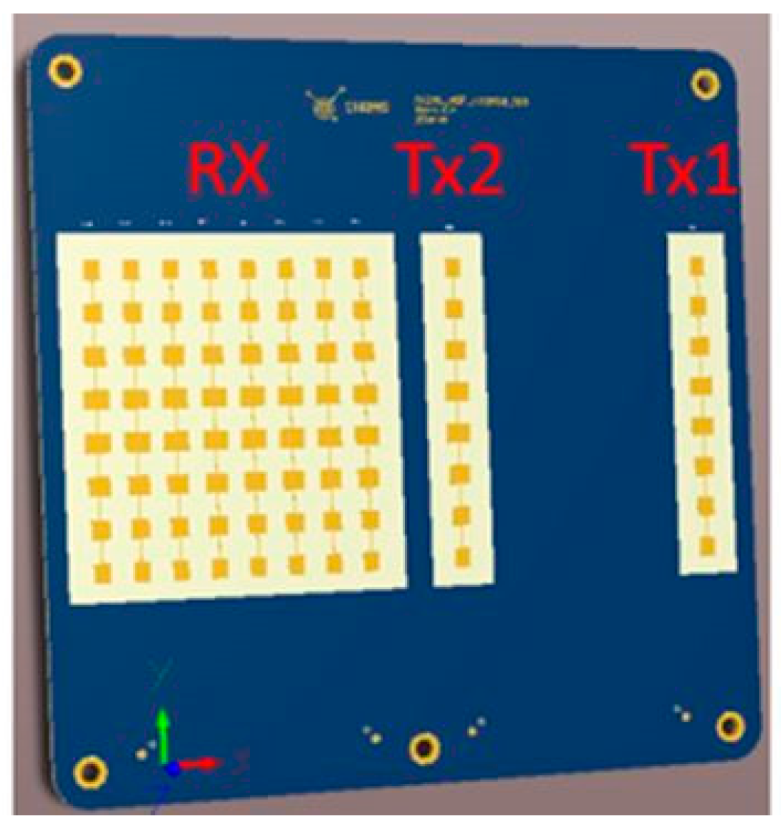
Figure 2.
Representation of the shadowing and tilt modulation effect in the vertical plane. The Tx/Rx antenna pair is located at quota H above the MSL. and delimit the radar FoV.
Figure 2.
Representation of the shadowing and tilt modulation effect in the vertical plane. The Tx/Rx antenna pair is located at quota H above the MSL. and delimit the radar FoV.

Figure 3.
Data processing chain for bathymetry map estimation.
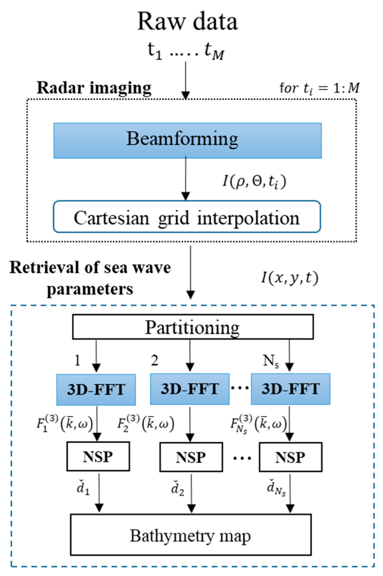
Figure 4.
Synthetic SWF1 at time . (a) Elevation profile. (b) Radar image.
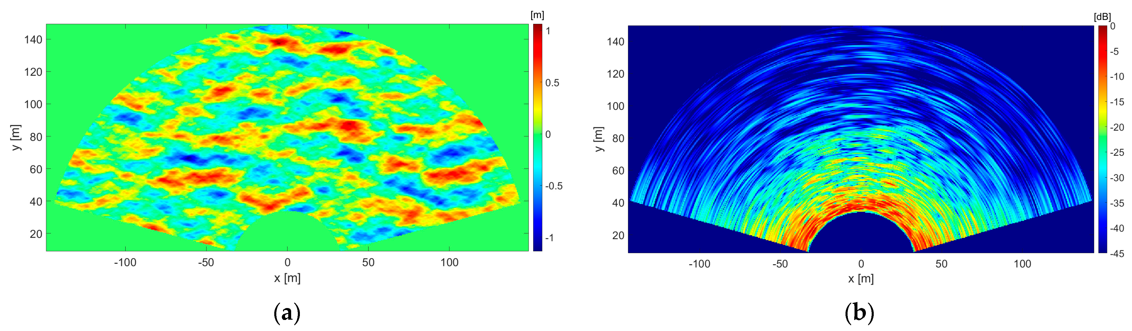
Figure 5.
(a) SNR map for SWF1 with, superimposed upon it, the black solid line enclosing the area where SNR ≥ 3dB. (b–d) Reconstructed bathymetry field for SWF1, SWF2, and SWF3, respectively.
Figure 5.
(a) SNR map for SWF1 with, superimposed upon it, the black solid line enclosing the area where SNR ≥ 3dB. (b–d) Reconstructed bathymetry field for SWF1, SWF2, and SWF3, respectively.
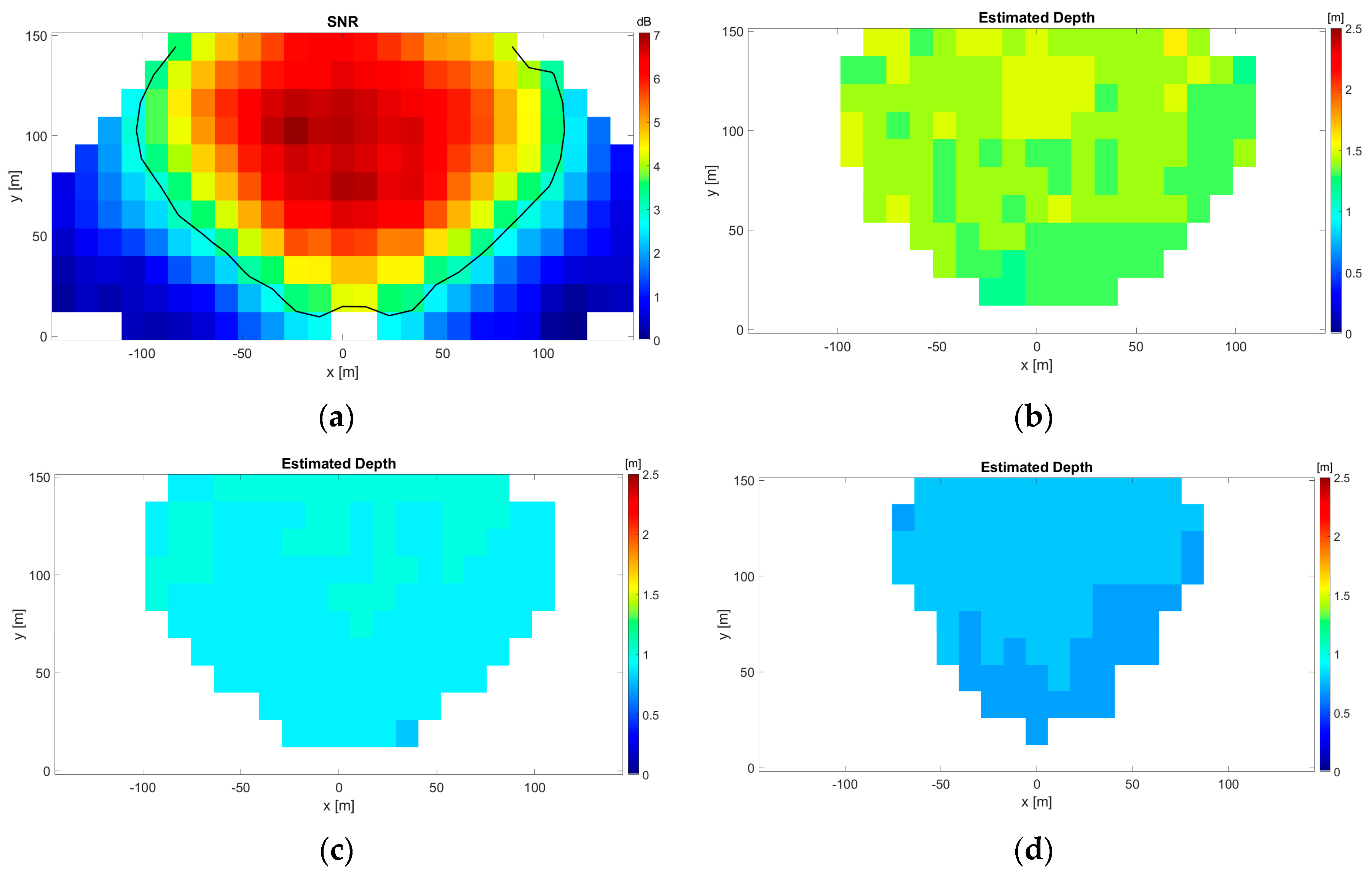
Figure 6.
Synthetic SWFPSB1 at time . (a) Sea waves propagating over the linear bathymetry. (b) Radar image.
Figure 6.
Synthetic SWFPSB1 at time . (a) Sea waves propagating over the linear bathymetry. (b) Radar image.
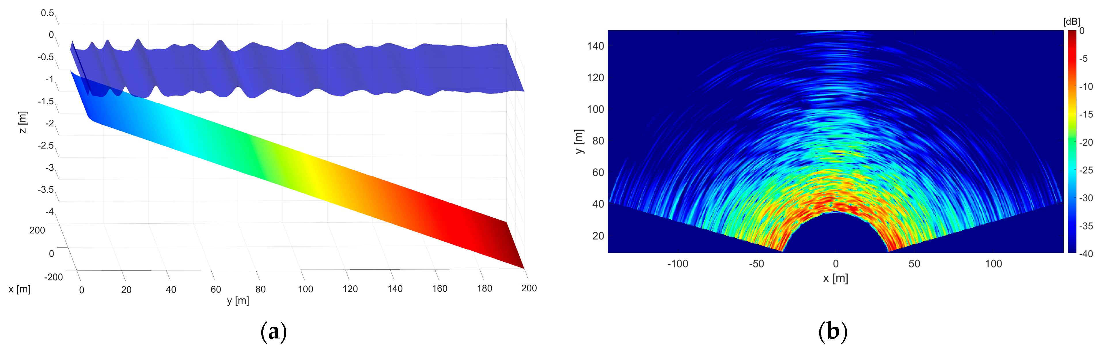
Figure 7.
(a–c) Bathymetry maps based on the SNR ≥ 3 dB criterion retrieved from SWFPSB1, SWFPSB2, and SWFPSB3, respectively.
Figure 7.
(a–c) Bathymetry maps based on the SNR ≥ 3 dB criterion retrieved from SWFPSB1, SWFPSB2, and SWFPSB3, respectively.
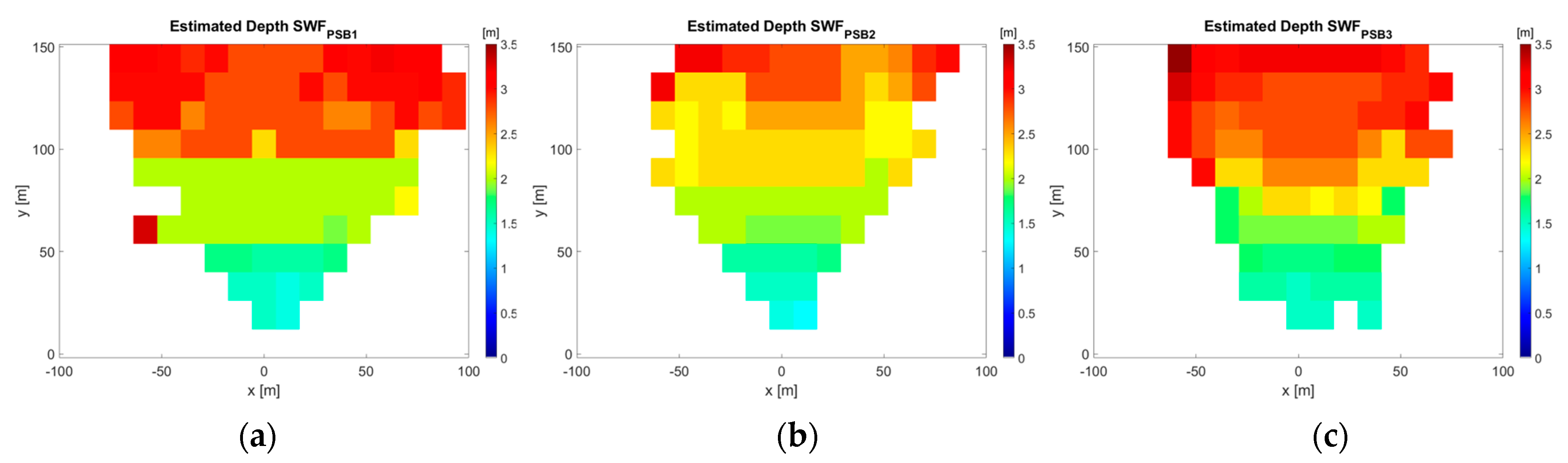
Figure 8.
Comparison between estimated bathymetry (dots) and ground truth (red dashed line). The equation of the regression line (black dashed line) is provided in the legend. (a–c) Scatterplot for SWFPSB1, SWFPSB2, and SWFPSB3, respectively.
Figure 8.
Comparison between estimated bathymetry (dots) and ground truth (red dashed line). The equation of the regression line (black dashed line) is provided in the legend. (a–c) Scatterplot for SWFPSB1, SWFPSB2, and SWFPSB3, respectively.
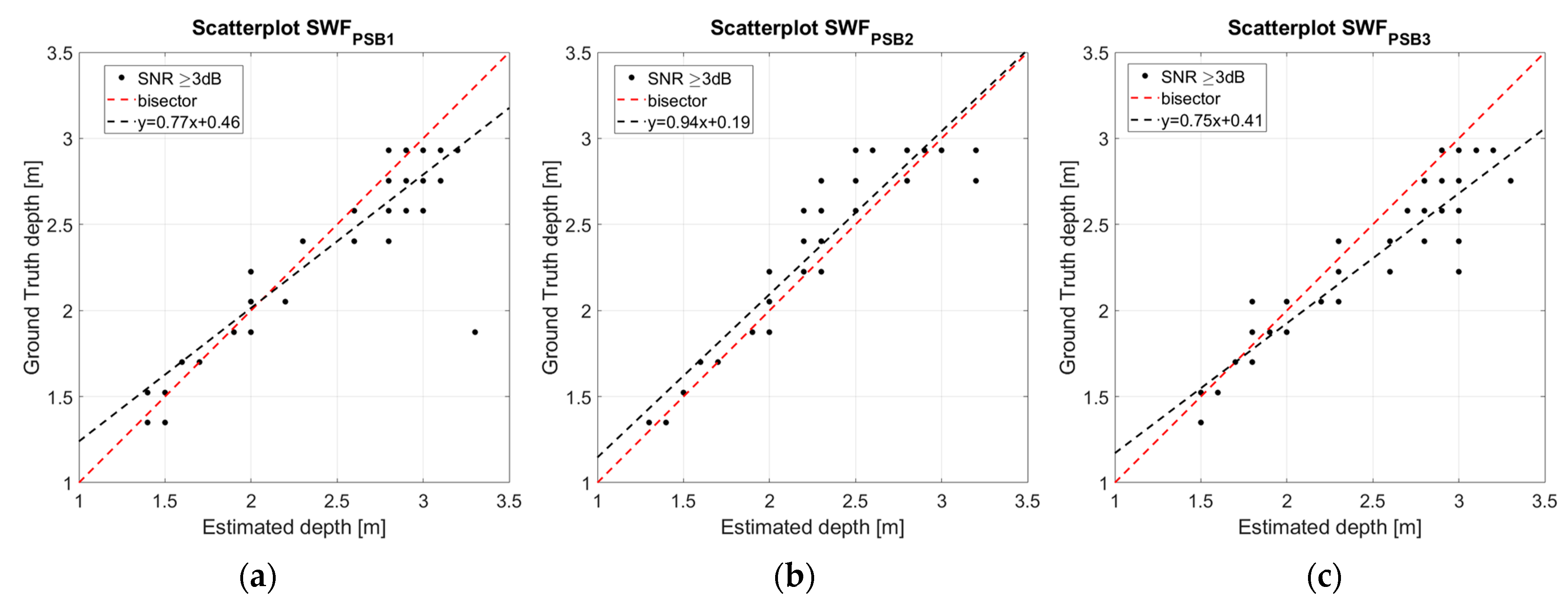
Figure 9.
Satellite image of the test site. The inset displays the radar’s positioning overlaid on a radar image. A1 and A2 show the location of two anemometric stations.
Figure 9.
Satellite image of the test site. The inset displays the radar’s positioning overlaid on a radar image. A1 and A2 show the location of two anemometric stations.
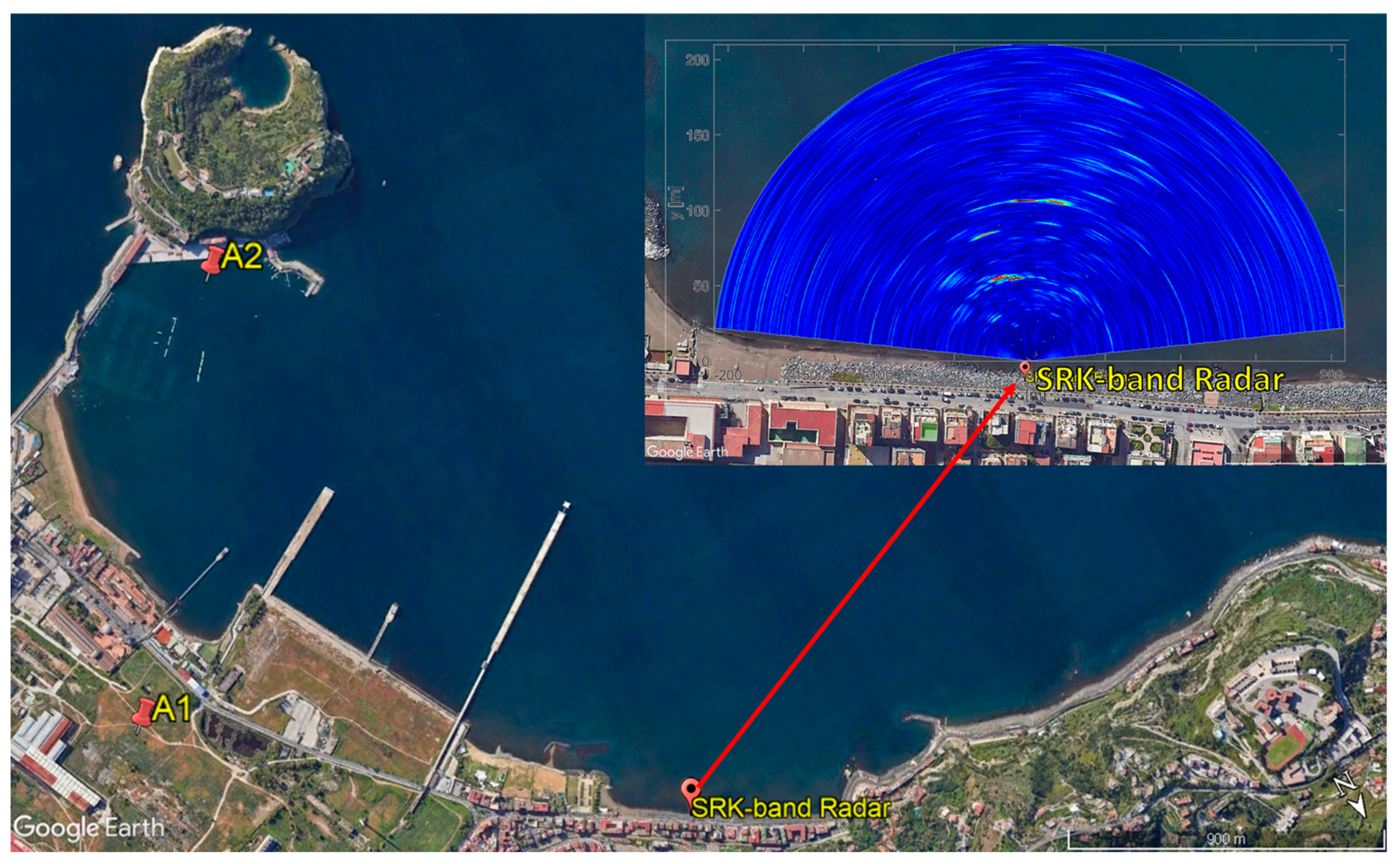
Figure 10.
(a) SRK-band radar system installation. (b) Cross-section of normalized 3D radar data spectrum (color scale [0,1]).
Figure 10.
(a) SRK-band radar system installation. (b) Cross-section of normalized 3D radar data spectrum (color scale [0,1]).

Figure 11.
(a) Bathymetry field estimated at Bagnoli Bay. The black solid line encloses the area where the SNR ≥ 3 dB. (b) Georeferenced SNR bathymetry field based on SNR ≥ 3dB criterion. The white line is the isobath at depth 2 m.
Figure 11.
(a) Bathymetry field estimated at Bagnoli Bay. The black solid line encloses the area where the SNR ≥ 3 dB. (b) Georeferenced SNR bathymetry field based on SNR ≥ 3dB criterion. The white line is the isobath at depth 2 m.


Table 1.
Main characteristic of SWFs.
| SWF1 | 1.5 | 1.54 | 0.24 | 1.21 | 20 |
| SWF2 | 1.0 | 1.82 | 0.33 | 0.86 | 12 |
| SWF3 | 0.8 | 2.08 | 0.44 | 0.71 | 8 |
Table 2.
Parameters defining the radar configuration.
| Parameter | Description | Value | Unit |
|---|---|---|---|
| fstart | Min. frequency | 24.00 | [GHz] |
| fstop | Max. frequency | 24.25 | [GHz] |
| Tc | Chirp duration | 200 | [μs] |
| PRF | Pulse repetition frequency | 2 | [Hz] |
| Nt | No. baseband samples | 1024 | - |
| fs | Baseband sampling frequency | 5 | [MHz] |
| Tw | Observation time window | 128 | [s] |
| AzFov | Azimuthal FoV | 150 | [°] |
| H | Radar height (above MSL) | 10 | m |
| Min. range (above MSL) | 34 | m | |
| x | Max. range (above MSL) | 149 | m |
Table 3.
MRPE values for estimated bathymetry with the SNR ≥ 3 dB criterion.
| SWF1 | 3.8 |
| SWF2 | 7.2 |
| SWF3 | 8.0 |
Table 4.
Main characteristic of SWFPSB.
| SWFPSB1 | 1.3 | 0.25 |
| SWFPSB2 | 1.7 | 0.35 |
| SWFPSB3 | 2.1 | 0.45 |
Table 5.
MRPE and R values for estimated bathymetry using the SNR ≥ 3 dB criterion.
| SWFPSB1 | 7.8 | 0.90 |
| SWFPSB2 | 5.6 | 0.91 |
| SWFPSB3 | 8.5 | 0.94 |
Disclaimer/Publisher’s Note: The statements, opinions and data contained in all publications are solely those of the individual author(s) and contributor(s) and not of MDPI and/or the editor(s). MDPI and/or the editor(s) disclaim responsibility for any injury to people or property resulting from any ideas, methods, instructions or products referred to in the content. |
© 2024 by the authors. Licensee MDPI, Basel, Switzerland. This article is an open access article distributed under the terms and conditions of the Creative Commons Attribution (CC BY) license (https://creativecommons.org/licenses/by/4.0/).
Share and Cite
MDPI and ACS Style
Ludeno, G.; Antuono, M.; Soldovieri, F.; Gennarelli, G. A Feasibility Study of Nearshore Bathymetry Estimation via Short-Range K-Band MIMO Radar. Remote Sens. 2024, 16, 261. https://doi.org/10.3390/rs16020261
AMA Style
Ludeno G, Antuono M, Soldovieri F, Gennarelli G. A Feasibility Study of Nearshore Bathymetry Estimation via Short-Range K-Band MIMO Radar. Remote Sensing. 2024; 16(2):261. https://doi.org/10.3390/rs16020261
Chicago/Turabian StyleLudeno, Giovanni, Matteo Antuono, Francesco Soldovieri, and Gianluca Gennarelli. 2024. "A Feasibility Study of Nearshore Bathymetry Estimation via Short-Range K-Band MIMO Radar" Remote Sensing 16, no. 2: 261. https://doi.org/10.3390/rs16020261
Note that from the first issue of 2016, this journal uses article numbers instead of page numbers. See further details here.