End-to-End Convolutional Network and Spectral-Spatial Transformer Architecture for Hyperspectral Image Classification

Abstract

Although convolutional neural networks (CNNs) have proven successful for hyperspectral image classification (HSIC), it is difficult to characterize the global dependencies between HSI pixels at long-distance ranges and spectral bands due to their limited receptive domain. The transformer can compensate well for this shortcoming, but it suffers from a lack of image-specific inductive biases (i.e., localization and translation equivariance) and contextual position information compared with CNNs. To overcome the aforementioned challenges, we introduce a simply structured, end-to-end convolutional network and spectral–spatial transformer (CNSST) architecture for HSIC. Our CNSST architecture consists of two essential components: a simple 3D-CNN-based hierarchical feature fusion network and a spectral–spatial transformer that introduces inductive bias information. The former employs a 3D-CNN-based hierarchical feature fusion structure to establish the correlation between spectral and spatial (SAS) information while capturing richer inductive bias and more discriminative local spectral-spatial hierarchical feature information, while the latter aims to establish the global dependency among HSI pixels while enhancing the acquisition of local information by introducing inductive bias information. Specifically, the spectral and inductive bias information is incorporated into the transformer’s multi-head self-attention mechanism (MHSA), thus making the attention spectrally aware and location-aware. Furthermore, a Lion optimizer is exploited to boost the classification performance of our newly developed CNSST. Substantial experiments conducted on three publicly accessible hyperspectral datasets unequivocally showcase that our proposed CNSST outperforms other state-of-the-art approaches.

1. Introduction

Hyperspectral images (HSIs) consist of hundreds of contiguous narrow spectral bands extending across the electromagnetic spectrum, from visible to near-infrared wavelengths [1], resulting in abundant SAS information. Effectively classifying SAS features is critical in HSI processing, which aims at categorizing the content of each pixel using a set of pre-defined classes. In recent years, HSIC has seen widespread adoption across various domains, including urban planning [2], military reconnaissance [3], agriculture monitoring [4], and ocean monitoring [5].

The advancement of deep learning (DL) in artificial intelligence has considerably improved the processing of remote sensing images. When compared with traditional machine learning techniques including support vector machines (SVMs) [6], morphological profiles [7], k-nearest neighbor [8], or random forests [9], DL-based approaches exhibit a powerful feature extraction capability, thus being able to learn discriminative and high-level semantic information. Therefore, DL-based techniques are extensively employed for HSIC [10]. For instance, a deep stacked autoencoder network has been suggested for the classification of HSIs by focusing on learning spectral features [11]. Chen et al. [12] employed a multi-layer deep neural network and a singular restricted Boltzmann machine for the purpose of capturing the spectral characteristics within HSI data. However, these approaches solely utilize spectral data information and overlook the importance of spatial-contextual information for enhancing classification performance. Hence, joint SAS feature extraction methods have been proposed to extract additional contextual semantic information from complex spatial structures, thus enhancing the model’s classification performance. Yang et al. [13] presented a two-branch SAS characteristic extraction network that employed a 1D-CNN for spectral characteristic extraction and a 2D-CNN for spatial characteristic extraction. The learned SAS information is linked and channeled into a fully connected (FC) layer, which extracts spectral–spatial characteristics to facilitate further classification. Yet, the 2D-CNN architecture could potentially result in the loss of spectral information within HSI. To proficiently capture SAS features, a 3D-CNN coupled with a regularization model has been proposed [14]. Roy et al. [15] combined a 2D-CNN and 3D-CNN to acquire spectral–spatial characteristics jointly represented from spectral bands using 3D-CNN, and then further learned spatial feature representations using 2D-CNN. Guo et al. [16] proposed a dual-view spectral and global spatial feature fusion network that utilized an encoder–decoder structure with channel and spatial attention to fully mine the global spatial characteristics, while utilizing a dual-view spectral feature aggregation model with a view attention for learning the diversity of the spectral characteristics and achieving a relatively good classification performance.

Despite the above CNN-based approaches achieving relatively good categorization results in the classification tasks, they did not exploit hierarchical SAS feature information across various layers. Furthermore, the excessive depth of convolutional layers may cause gradient vanishing and explosion problems. The dense connected convolutional network (DenseNet) offers an effective solution to mitigate these issues; it achieves this by promoting the maximal flow of information among different convolutional layers through connectivity operations, effectively fusing the hierarchical features between different layers [17]. Based on this, a comprehensive deep multi-layer fusion DenseNet using 2D and 3D dense blocks was presented in [18], which effectively improved the exploitation of HSI hierarchical signatures and handled the gradient vanishing problem. In [19], a fast dense spectral–spatial convolution network (FDSSC) was introduced, which combines two separate dense blocks and increases the network’s depth, allowing for a more straightforward utilization of feature information across different layers. By combining the advantages of CNN and graph convolutional network (GCN), Zhou et al. [20] proposed an attention fusion network based on multiscale convolution and multihop graph convolution to extract multi-level complex SAS features of HSI. Liang et al. [21] presented a framework that integrates a multiscale DenseNet with bidirectional recurrent neural networks, which adopted the multiscale DenseNet (instead of traditional CNNs) to strengthen the utilization of spatial characteristics across different convolutional layers. Despite the powerful ability of the above DenseNet-based approaches to retrieve SAS characteristics in HSI classification tasks, they still suffer from the limitation that CNNs typically only consider local SAS information between features, while ignoring global SAS information (failing to establish global dependencies across long-range distances among HSI pixels).

Recently, vision transformers have witnessed a surge in popularity within numerous facets of computer vision, including target recognition, image classification, and instance segmentation [22,23]. Transformers are primarily composed of numerous self-attention and feed-forward layers that inherit the global receptive field, which allows them to efficiently establish long-range dependencies among HSI pixels, compensating for the lack of CNNs in global feature extraction. Hence, vision transformers have attracted widespread attention in HSIC, in which the MHSA serves as the primary characteristic extractor of the transformer for learning the remote locations of HSI pixels and global dependencies between spectral bands [24,25]. Furthermore, the transformer emphasizes prominent features while concealing less significant information. He et al. [26] were pioneers in developing a bi-directional encoder representation of the transformer-based model for establishing global dependencies in HSIC. This approach primarily relies on the MHSA mechanism of the MHSA layer, where each head encodes a global contextual semantic-aware representation of the HSI for discriminative SAS characteristics. Hong et al. [27] proposed a framework for learning the long-range dependence information between spectral signatures using group spectral embedding and transform encoders by treating HSI data as sequential information, while fusing “soft” residuals across layers to mitigate the loss of critical signature information in the process of hierarchical propagation. Xue et al. [28] introduced a local transformer model in combination with the spatial partition restore network, which can effectively acquire the HSI global contextual dependencies and dynamically acquire the spatial attention weights through the local transformer to adapt to the intrinsic changes in HSI spatial pixels, thus augmenting the model’s ability to retrieve spatial–contextual pixel characteristics. Mei et al. [29] introduced a group-aware hierarchical transformer (GAHT) for HSIC, which incorporates a new group pixel embedding module that highlights local relationships in each HSI spectral channel, thus modeling global–local dependencies from a spectral–spatial point of view.

Although the above transformer-based models exhibit excellent abilities to model long-range dependencies among HSI pixels, they still suffer from some limitations in terms of extracting HSI characteristic information: (1) MHSA falls short in effectively considering both the positional and spectral information of the input HSI blocks when establishing the global dependencies of the HSI, which renders that the network lacks the utilization of the positional information among HSI pixels, and (2) some discriminative local SAS characteristic information that is helpful for HSIC purposes is not sufficiently exploited. Given that CNNs exhibit strong local characteristic learning abilities, a convolutional transformer (CT) network was proposed in [30], first employing central position coding to merge the spectral signatures and pixel positions to obtain the spatial positional signatures of the HSI patches, and then utilizing the CT block (containing two 2D-CNNs with 3 × 3 convolutional kernel sizes) to acquire the local–global characteristic information of HSIs, which significantly improved this model’s local–global feature acquisition ability. The spectral–spatial feature tokenization transformer (SSFTT) was introduced in [31], which converts the SAS characteristics learned by a simple 3D-CNN and 2D-CNN layer into semantic tokens, and inputs them into a transformer encoder to perform spectral–spatial characteristic representation. Although the above methodologies try to employ CNNs to strengthen the local characteristic extraction capabilities of the network, the simple CNN structure fails to adequately extract hierarchical features in various network layers. In this regard, Yan et al. [32] proposed a hybrid convolutional and ViT network classification approach, where one branch uses hybrid convolution and ViT to boost the capability of acquiring local–global spatial characteristics, and the other branch utilizes 3D-CNNs to retrieve spectral characteristics. However, separate extraction of SAS characteristics with a branch based on 2D-CNNs and a hybrid convolutional transformer network based on 3D-CNNs may ignore the intrinsic correlation between SAS signatures. A local semantic feature aggregation-based transformer approach was proposed in [33], which utilizes 3D-CNNs to simultaneously extract shallow spectral–spatial characteristics, and then merges pixel-labeled features using a local pixel aggregation operation to provide multi-scale characteristic neighborhood representations for HSIC. A two-branch bottleneck spectral–spatial transformer (BS2T) method was introduced in [34], which utilizes two 3D-CNNs DenseNet structures to separately abstract SAS properties to boost the extraction of the localized characteristics, as well as two transformers for establishing the long-range dependencies between HSI pixels. However, it may result in the model failing to adequately leverage the correlation between SAS information (this architecture contains two 3D-CNNs hierarchical structures and two transformers, and is relatively complex). Zu et al. [35] proposed exploiting a cascaded convolutional feature token to obtain joint spectral–spatial information and incorporate certain inductive bias properties of CNNs into the transformer. The densely connected transformer is then utilized to improve the characteristic propagation, significantly boosting the model’s performance.

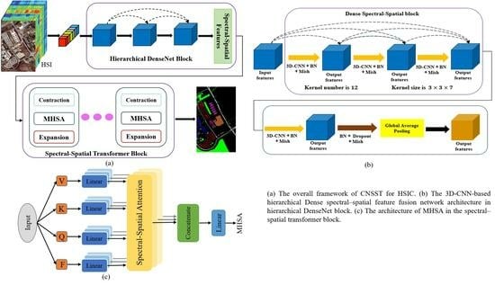
Inspired by the above, we propose a simply structured, end-to-end convolutional network and spectral–spatial transformer (CNSST) architecture for HSIC. It comprises two primary modules, a 3D-CNN-based hierarchical feature fusion network and a spectral–spatial transformer that introduces inductive bias properties information (i.e., localization, contextual position, and translation equivariance), which are used to boost the extraction of local feature information and establish global dependencies, respectively. Regarding the local spectral–spatial feature extraction, to acquire SAS hierarchical characteristic representations with more rich inductive bias information, a 3D-CNN-based hierarchical network strategy is utilized to capture SAS information simultaneously, so as to establish the correlation between the SAS information of HSI pixels and to obtain a more rich inductive bias (yet more discriminative spectral–spatial joint feature information). Meanwhile, the hierarchical feature fusion structure is utilized to boost the utilization of the HSI semantic feature information across different convolutional layers. In the spectral–spatial transformer network, the SAS hierarchical characteristics containing rich inductive bias information are introduced into the MHSA to make up for the shortcoming of insufficient inductive bias in the image features acquired by the transformer. This allows the transformer not only to effectively establish long-range dependencies among HSI pixels, but also to enhance the model’s location-aware and spectral-aware capabilities. Moreover, a Lion optimizer is exploited to enhance the performance of the model. A summary of the primary contributions of this research is as follows:

• We propose a simply structured, end-to-end convolutional network and spectral–spatial transformer (CNSST) architecture based on a 3D-CNN hierarchical feature fusion network and a spectral–spatial transformer that introduces rich inductive bias information in the HSI classification process.
• To obtain feature representations with richer inductive bias information, a 3D-CNN-based hierarchical network is utilized to capture SAS information simultaneously in order to establish the correlation between these two sources of information in HSI pixels, while the hierarchical structure is exploited to improve the utilization of the HSI semantic feature information in various convolutional layers.
• Spectral–spatial hierarchical features containing rich inductive bias information are introduced into MHSA, which enables the transformer to effectively establish long-range dependencies among HSI pixels, and to be more location-aware and spectral-aware. Moreover, a Lion optimizer is exploited to boost the categorization performance of the network.

The rest of this article is structured as follows. The related work is briefly described in Section 2. Section 3 provides an in-depth description of the general framework of the CNSST. Section 4 shows the experimental analysis and discussion. Finally, Section 5 wraps up the paper with concluding remarks and hints at future research directions.

2. Related Work

This section provides an introduction of the basic modules used in our CNSST architecture, including 3D-CNNs, hierarchical DenseNet, and the self-attention mechanism.

2.1. 3D-CNNs for HSI Classification

Here, 1D-CNNs can be applied to extract spectral signatures of HSI pixels, and 2D-CNNs are normally utilized to obtain spatial information. Yet, there is abundant SAS information contained in HSIs, which means that separate extraction of SAS characteristics may ignore the correlation between certain spatial characteristics and specific spectral characteristics. Compared with traditional pixel-based approaches, 3D-CNN-based approaches employ the target pixel and its neighboring pixels as inputs, which makes it possible to capture the rich spatial information surrounding the target pixel and fully leverages the correlation between SAS information, whereas pixel-based approaches solely employ a single pixel for network training. The input size of the 3D-CNN-based approach is p × p × b, where p × p and b stand for the number of neighboring pixels and spectral bands, respectively. Consequently, 3D-CNN is utilized as the foundational structure of the proposed CNSST model to obtain SAS feature information to fully capitalize on the correlation between certain spatial features and specific spectral features.

The inclusion of batch normalization in 3D-CNN modules is a common tool used in DL models to make the learning process fast and to reduce the dependence on initial values [36]. As a result, a batch normalization (BN) layer is incorporated into each 3D-CNN layer to increase numerical stability and suppress overfitting. As demonstrated in Figure 1, $n_i$ feature map (FM) of size $p_i\times p_i\times b_i$ is input into a 3D-CNN layer containing $m_{i+1}$ channels sized ${\alpha }_{i+1}\times {\alpha }_{i+1}\times d_{i+1}$, resulting in $n_{i+1}$ output FM of size $p_{i+1}+p_{i+1}+b_{i+1}$. The ith output of the $(i+1)$-th 3D-CNN layer with BN output can be computed as follows:

$$X_k^{i+1}=Af\left(\sum _{j=1}^{n_i}\frac{{X_j}^i-Ex\left(X_j^i\right)}{Vf\left(X_j^i\right)}\ast H_k^{i+1}+b_k^{i+1}\right),$$

(1)

where $Af(·)$ represents the activation function (AF) employed to introduce nonlinear properties to boost the representation of the network. The jth input FM of the $(i+1)$-th layer is denoted as $X_j^i\in R^{P\times P\times b}$, while $Ex(·)$ and $Vf(·)$ correspond to the expectation and variance function of the input feature tensor, separately. $H_k^{i+1}$ and $b_k^{i+1}$ stand for the weight parameters and bias values of the $(i+1)$-th 3D-CNN layer, respectively, while ∗ stands for the convolution operation.

2.2. Hierarchical DenseNet

Traditional CNNs merely transform FMs forward from one convolutional layer to the next one. They are unable to train the network using information from different layers. Typically, increasing the number of convolutional layers tends to enhance the network performance. However, an excessive number of layers may result in gradient disappearing and explosion problems. The hierarchical Densenet is used to effectively mitigate these issues. It connects each layer directly to the other ones and combines features in the channel dimension by concatenating them to ensure maximum information flow between layers. Every convolutional layer receives information from the preceding layer as an input and subsequently transmits its FM to the succeeding layer [17]. The architecture of the hierarchical DenseNet is depicted Figure 2. The dense block serves as the fundamental unit in the hierarchical DenseNet. Assuming that the lth layer’s output FM is $x_l$, the output of the l-th layer’s dense block may be represented as follows:

$$x_l=H_l\left[x_0,x_1,\cdots ,x_{l-1}\right],$$

(2)

where $H_l(·)$ denotes a functional module that comprises BN layers, convolution layers, and Mish AF layers. Additionally, $x_0,x_1,\cdots ,x_{l-1}$ denote the output FMs of the previous dense blocks.

The architecture of the dense block employed in our model is presented in Figure 3. Specifically, each convolutional layer consists of m kernels of shape $\alpha \times \alpha \times d$. Each layer then produces m FMs with dimensions $p\times p\times b$. The number of FMs corresponds to the number of convolutional kernels and a linear correlation exists between the number of channels in each layer and the convolutional layers. The number of channels $m_j$ in the dense block of the jth layer takes the value $(j-1)\times m+b$, with b representing the number of channels from the input FMs.

2.3. Self-Attention Mechanism

Attention mechanisms have their origins in the investigation of the human visual nervous system, which has always been able to selectively concentrate on the significant parts of all information, while ignoring other irrelevant parts. The same is true for the attention mechanism in DL. The self-attention mechanism (SA) has revolutionized various natural language processing (NLP) tasks by capturing dependencies and relationships among various elements in a sequence. It enables models to assess the significance of different elements dynamically, resulting in improved performance on tasks, including text translation [37], sentiment analysis [38], and NLP [39]. In the domain of HSIC, SA has also been widely exploited [26,27,28,29,30,31]. The SA can be represented as:

$$Attention(Q,K,V)=S(\frac{Q{K}^T}{\sqrt{d_K}})V,$$

(3)

where $S(·)$ denotes the softmax AF. Q, K, V, and $d_K$ represent the query, key, value, and dimension of the value K, correspondingly. The query holds the information to be extracted, the keyword serves as the index, and the value encapsulates the feature to be fetched. Attention is computed by obtaining the correlation between the query and the key, obtaining the attention graph, which is then utilized to derive the eigenvalues of the values. Figure 4 illustrates the detailed architecture of the SA. In HSIC, SA exhibits superior discrimination. Ge et al. [40] combined multiscale pyramidal convolutional blocks and polarized attention blocks to retrieve SAS characteristics from HSIs. Xia et al. [41] introduced a lightweight residual structure to replace the standard residual structure. This structure introduces an SA, enabling adaptive fusion of the input and output FMs, thereby further enhancing the feature extraction capability of the residual structure. [42] developed a novel high-order self-attention network that utilizes the SA module to capture long-range dependencies within scenes, facilitating the extraction of high-level semantic features. In the proposed method, to enhance the transformer’s location and spectral awareness, a novel MHSA with position coding is used to characterize the spatial location correlation and spectral–spatial correlation among hierarchical spectral–spatial features that contain rich induced bias information.

3. Methodology

The structure of the proposed CNSST model is schematically depicted in Figure 5. The CNSST architecture is formed by two primary components: a 3D-CNN-based hierarchical feature fusion network and a spectral–spatial transformer network that introduces inductive bias properties information. In terms of the 3D-CNN-based hierarchical feature fusion network, the 3D-CNN-based hierarchical network strategy is employed to capture SAS information simultaneously, so as to establish the correlation among the SAS information of the HSI and to obtain more abundant inductive bias. Moreover, the hierarchical DenseNet feature fusion structure is utilized to promote the utilization of the HSI semantic characteristic information in the respective convolutional layers, aiming to achieve a spectral–spatial hierarchical signature representation with richer inductive bias information. The spectral–spatial transformer network is employed to establish long-range dependencies between HSI pixels and to reinforce the local characteristic extraction capability. Specifically, the spectral–spatial hierarchical signatures containing rich inductive bias information are introduced into the multi-head spectral–spatial self-attention module to make up for the shortcomings of insufficient inductive bias in the image features acquired by the transformer, as well as to make the model more location-aware and spectral-aware. Finally, spectral–spatial feature fusion is conducted by the FC layer and then the probability prediction of each class is conducted by the Softmax AF. Moreover, a Lion optimizer is exploited to improve the categorization performance of the model. Next, we describe each of the modules in detail.

3.1. 3D-CNN-Based Hierarchical Dense Spectral-Spatial Feature Fusion Network

In this section, we provide a detailed description of the 3D-CNN-based hierarchical dense spectral–spatial feature fusion network module in CNSST. As shown in Figure 6, the structure primarily consists of a 3D-CNN-based hierarchical DenseNet spectral–spatial block. Unlike methods that obtain SAS characteristics by spectral branch and spatial branch, respectively, here, a 3D-CNN-based hierarchical DenseNet is adopted to extract the spectral–spatial characteristics simultaneously in order to establish the correlation between SAS information while capturing richer inductive bias and more discriminative local SAS hierarchical characteristic information. When the pixels containing abundant spectral–spatial characteristic information are introduced into the proposed structure, the proposed model with multiple nonlinear layers can effectively provide hierarchical feature representations. Furthermore, the utilization of multiple convolutional layers enables CNN to learn features more discriminatively under sparsity constraints. Regarding the network parameter settings, assuming that the input FM is of size $H\times W\times D$ with n channels, and the convolution layer comprises $m_o$ kernels with size $a_o\times a_o\times d_o$, then each layer calculates FMs as follows:

$$H_o=\frac{H+2P_{ad}-a_o}{s_o+1},$$

(4)

$$W_o=\frac{W+2P_{ad}-a_o}{s_o+1},$$

(5)

$$D_o=\frac{D+2P_{ad}-d_o}{s_o+1},$$

(6)

where $H_o,W_o$, and $D_o$ represent the corresponding sizes of the produced FMs. Parameter $P_{ad}$ denotes the padding applied during the resizing of the output FM, while $s_o$ signifies the stride of the filter used. Moreover, the corresponding number of channels within the resulting feature map can be expressed by $n+(j-1)\times m_o$, in which j pertains to the jth convolutional layer under consideration.

Specifically, the 3D-CNN-based hierarchical Dense spectral–spatial feature fusion model mainly consists of 4 convolutional layers, where each layer has a kernel size of $3\times 3\times 7$ and number of channels $m_o$ set to 12. In addition, we added a dropout layer between the last BN layer and the global average pooling layer to prevent overfitting. AF can enhance the efficiency of the counter-propagation and facilitate the network’s convergence. As shown in Figure 6, we adopted a self-regularized non-monotone AF Mish, which can preserve negative inputs as negative outputs, thereby effectively trading the input information and network sparsity. In the end, the local spectral–spatial characteristics extracted from the hierarchical dense spectral–spatial feature fusion network containing rich inductive bias and more discriminative characteristics are used as the inputs to the spectral–spatial transformer block.

3.2. Spectral–Spatial Transformer Network

As illustrated in Figure 5, the proposed spectral–spatial transformer block primarily contains a spectral–spatial MHSA module, as well as feature contraction and expansion modules. The MHSA module feeds the feature mapping into the spectral–spatial transformer module, which contains rich induced bias and hierarchical spectral–spatial characteristics, and then utilizes the spectral–spatial self-attention and positional coding modules to establish the global remote dependencies of the spectral–spatial characteristics in HSI pixels. To be specific, in the spectral–spatial transformer block, spectral–spatial hierarchical characteristics of size $H_o\times W_o\times D_o$ are first fed into the feature contraction module consisting of convolutions with a convolution kernels of size $1\times 1$ and BN operations. Following that, the new characteristics obtained after feature contraction are input into the MHSA module to establish long-range dependencies between the HSI pixels. Finally, the convolution kernel with a size of $1\times 1$ is employed in the feature expansion module for the dimensionality change, so the output features can be adapted to the structure of the network and are better combined between different levels of FMs.

Generally, positional coding is employed as a constraint to boost the attention sensitivity to positional information in transformer-based approaches [34,35]. Relative distance-aware position coding has great potential for describing the spatial content location of image pixels. The reason for this is that the attention considers not only the contextual feature information, but also the relative distances between the different positional features in pixels, which can effectively establish the correlation between the image feature information and positional awareness [43]. Hence, in our proposed CNSST, we used 2D relative position self-attention to realize the relative position encoding of HSI pixel features. The 2D relative height information $L_h$ and relative width information $L_w$ are computed for each HSI pixel feature to obtain a new spectral–spatial feature $F_N$ containing the relative position information.

In addition, MHSA is a mapping process that converts a query and a set of key–value pairs into an output. In this process, each input (query, key, and value) is represented as a vector and the output is a weighted sum of the values. The architecture of MHSA in the spectral–spatial transformer is presented in Figure 7. To enhance the location-awareness and spectral-awareness of the proposed CNSST, MHSA with relative position coding is utilized to co-describe the spatial–positional and spectral–spatial correlations between the HSI pixel patches. Firstly, the HSI pixel features F are processed by three convolutional layers to yield three new groups of features $Q,K,V\in R^{H\times W\times D}$. Meanwhile, the entire hierarchical spatial features on the channel are mapped to global features, utilizing the global pooling operation to produce the spectral signatures $F_o$ of $F_N$, which are then introduced into the attention mechanism, where the spectral–spatial attention $AM$ can be represented as follows:

$$AM=Attention(Q,K,V,F_o)=S\left(\frac{(L_h+L_w)Q{K}^T}{\sqrt{d_k}}\right)F_{o}V,$$

(7)

where $S(·)$ denotes the softmax AF. $L_h$ and $L_w$ stand for the height information and width information of the 2D relative position encoding, respectively. Q, K, V, $F_o$, and $d_K$ correspond to the query, key, value, spectral signatures, and dimension of the value K, correspondingly. These weight matrices and parameters were utilized to calculate MHSA, and the outcomes from each attention head are concatenated to obtain the output MHSA with H-heads, which can be expressed as follows:

$$MHSA(Q,K,V,F_o)=Concat(A{M}_1,A{M}_2,\cdots ,A{M}_H)W,$$

(8)

where W signifies the matrix parameters obtained from the linear layers, and H signifies the number of heads.

3.3. Lion Optimizer

The optimizer has a significant role in training DL models, and its primary aim is to help the model gradually learn and update the parameters to make it fit the data better and decrease its loss function. The Lion optimizer is a simple and efficient optimization algorithm, and it has achieved excellent performance in image classification, computer vision, and other areas [44]. Unlike traditional optimizers, that store 1st and 2nd order moments, Lion merely tracks momentum and utilizes symbolic function operations for calculating parameter updates, thereby not only boosting the performance of the model, but also reducing memory overhead. To improve the categorization performance of CNSST, the Lion optimizer is applied to the CNSST model instead of the traditional Adam optimizer. The Lion optimizer’s computational procedure can be expressed as follows:

$$g_t={▽}_{\vartheta }f\left({\vartheta }_{t-1}\right),$$

(9)

$${\vartheta }_t={\vartheta }_{t-1}-{\psi }_t\{sign[{\rho }_1{m}_{t-1}+(1-{\rho }_1)g_t]+\lambda {\vartheta }_{t-1}\},$$

(10)

$$m_t={\rho }_2{m}_{t-1}+(1-{\rho }_2)g_t,$$

(11)

where $g_t={▽}_{\vartheta }f\left({\vartheta }_{t-1}\right)$ is denoted as the gradient of the loss function at weight ${\vartheta }_{t-1}$ for the current sample. Equation (10) represents the weight reduction process of decoupling, in which ${\psi }_t$ denotes the step size and $sign(·)$ denotes the sign function. ${\rho }_1$ and ${\rho }_2$ denote the decay rates of the 1st and 2nd order moments, respectively, and their corresponding default values are set to 0.9 and 0.99. $m_t$ is the momentum vector of the t-th iteration. Equation (11) is employed for calculating the bias-corrected 1st and 2nd moments to offset the bias.

4. Experiments and Analysis

To assess the efficacy of the proposed CNSST approach, intensive experiments are performed using three familiar HSIC datasets. Next, we describe the datasets utilized, experimental settings, and then compare and experimentally analyze them in conjunction with several state-of-the-art models to exemplify the validity of the CNSST.

4.1. Datasets Description

In the experimental evaluations, four HSIC datasets are adopted to assess the CNSST approach we introduced. These datasets include the University of Pavia (UP), Salinas Scene (SV), Indian Pines (IP), and ZaoYan region (ZY). The corresponding pseudo-color and ground-truth images for these three datasets are depicted in Figure 8. Details about the categories and samples of the counterpart datasets are provided in Table 1, Table 2, Table 3 and Table 4. The details are shown below:

UP: It was acquired utilizing the ROSIS-3 sensor through an aerial survey performed over the Pavia region, Italy. It includes $610\times 340$ pixels, containing a combined count of 42,776 labeled samples distributed among 9 distinct classes. Notably, this dataset encompasses 103 spectral bands, spanning a wavelength range from 4.3 $\mathsf{\mu }\mathrm{m}$ to 8.6 $\mathsf{\mu }\mathrm{m}$.

SV: It was gathered utilizing the AVIRIS sensor—equipped with 224 spectrum bands—over Salinas Valley, USA. The dimensions of the images within this dataset are $512\times 217$ pixels. It contains 54,129 sample pixels labeled samples distributed among 16 distinct classes and encompasses 204 bands in the range of 0.4 $\mathsf{\mu }\mathrm{m}$ to 2.5 $\mathsf{\mu }\mathrm{m}$ wavelengths.

IP: It was gathered utilizing the AVIRIS sensor over the region of Indiana, USA. It includes 16 distinct classes in total, spanning a wavelength ranging from 0.4 $\mathsf{\mu }\mathrm{m}$ to 2.5 $\mathsf{\mu }\mathrm{m}$. The scene’s dimensions encompass $145\times 145$ pixels, 220 spectral bands, and a combined count of 10,249 samples are available within this dataset.

ZY: It was collected by the OMIS sensor over the Zaoyuan region, China. The sense contained $137\times 202$ pixels and 80 spectral bands with the first 64 spectral bands in the range of 0.4 $\mathsf{\mu }\mathrm{m}$ to 1.1 $\mathsf{\mu }\mathrm{m}$ and the last 16 covering the region of 1.06 $\mathsf{\mu }\mathrm{m}$ to 1.7 $\mathsf{\mu }\mathrm{m}$. The available ground-truth map contains only 23,821 labeled samples and 8 landcover classes.

Figure 8. Pseudo-color and ground-truth images of three datasets. Pseudo-color images of the UP, SV, IP, and ZY datasets are depicted in (a,c,e,g), while the counterpart ground-truth maps are displayed in (b,d,f,h).

Figure 8. Pseudo-color and ground-truth images of three datasets. Pseudo-color images of the UP, SV, IP, and ZY datasets are depicted in (a,c,e,g), while the counterpart ground-truth maps are displayed in (b,d,f,h).

Table 1. Details of the categories and sample numbers for UP dataset.

Category	Name	Total Number	Category	Name	Total Number
N1	Asphalt	6631	N6	Bare Soil	5029
N2	Meadows	18,649	N7	Bitumen	1330
N3	Gravel	2099	N8	Self-Blocking Bicks	3682
N4	Trees	3064	N9	Shadows Bare Soil	947
N5	Painted metal sheets	1345

Table 1. Details of the categories and sample numbers for UP dataset.

Category	Name	Total Number	Category	Name	Total Number
N1	Asphalt	6631	N6	Bare Soil	5029
N2	Meadows	18,649	N7	Bitumen	1330
N3	Gravel	2099	N8	Self-Blocking Bicks	3682
N4	Trees	3064	N9	Shadows Bare Soil	947
N5	Painted metal sheets	1345

Table 2. Details of the categories and sample numbers for SV dataset.

Category	Name	Total Number	Category	Name	Total Number
N1	Broccoli-green-weeds-1	2009	N9	Soil-vinyard-develop	6203
N2	Broccoli-green-weeds-2	3726	N10	Corn-senesced-green-weeds	3278
N3	Fallow	1976	N11	Lettuce-romaine-4wk	1068
N4	Fallow-rough-plow	1394	N12	Lettuce-romaine-5wk	1927
N5	Fallow-smooth	2678	N13	Lettuce-romaine-6wk	916
N6	Stubble	3959	N14	Lettuce-romaine-7wk	1070
N7	Celery	3579	N15	Vinyard-untrained	7268
N8	Grapes-untrained	11,271	N16	Vinyard-vertical-trellis	1807

Table 2. Details of the categories and sample numbers for SV dataset.

Category	Name	Total Number	Category	Name	Total Number
N1	Broccoli-green-weeds-1	2009	N9	Soil-vinyard-develop	6203
N2	Broccoli-green-weeds-2	3726	N10	Corn-senesced-green-weeds	3278
N3	Fallow	1976	N11	Lettuce-romaine-4wk	1068
N4	Fallow-rough-plow	1394	N12	Lettuce-romaine-5wk	1927
N5	Fallow-smooth	2678	N13	Lettuce-romaine-6wk	916
N6	Stubble	3959	N14	Lettuce-romaine-7wk	1070
N7	Celery	3579	N15	Vinyard-untrained	7268
N8	Grapes-untrained	11,271	N16	Vinyard-vertical-trellis	1807

Table 3. Details of the categories and sample numbers for the IP dataset.

Category	Name	Total Number	Category	Name	Total Number
N1	Alfalfa	46	N9	Oats	20
N2	Corn-notill	142	N10	Soybean-notill	972
N3	Corn-mintill	830	N11	Soybean-mintill	2455
N4	Corn	237	N12	Soybean-clean	593
N5	Grass-pasture	483	N13	Wheat	205
N6	Grass-trees	730	N14	Woods	1265
N7	Grass-pasture-mowed	28	N15	Buildings-Grass-Trees-Drives	386
N8	Hay-windrowed	478	N16	Stone-Steel-Towers	93

Table 3. Details of the categories and sample numbers for the IP dataset.

Category	Name	Total Number	Category	Name	Total Number
N1	Alfalfa	46	N9	Oats	20
N2	Corn-notill	142	N10	Soybean-notill	972
N3	Corn-mintill	830	N11	Soybean-mintill	2455
N4	Corn	237	N12	Soybean-clean	593
N5	Grass-pasture	483	N13	Wheat	205
N6	Grass-trees	730	N14	Woods	1265
N7	Grass-pasture-mowed	28	N15	Buildings-Grass-Trees-Drives	386
N8	Hay-windrowed	478	N16	Stone-Steel-Towers	93

Table 4. Details of the categories and sample numbers for ZY dataset.

Category	Name	Total Number	Category	Name	Total Number
N1	Vegetable	2625	N5	Corn	1425
N2	Grape	1302	N6	Terrace/Grass	1484
N3	Dry vegetable	3442	N7	Bush-Lespedeza	1808
N4	Pear	10,243	N8	Peach	1492

Table 4. Details of the categories and sample numbers for ZY dataset.

Category	Name	Total Number	Category	Name	Total Number
N1	Vegetable	2625	N5	Corn	1425
N2	Grape	1302	N6	Terrace/Grass	1484
N3	Dry vegetable	3442	N7	Bush-Lespedeza	1808
N4	Pear	10,243	N8	Peach	1492

4.2. Experimental Settings

To better compare the classification performance (experimental classification accuracy and classification visual maps) of different methods, during the selection of experimental training data, 1% of labeled samples are uniformly chosen for training from the UP and SV datasets, which contain a substantial number of labeled samples (42,776 and 54,129 labeled samples), while the remainder is for testing. However, for the IP and ZY datasets, which have relatively fewer labeled samples (10,249 and 23,821 labeled samples), 10% and 2.5% of the samples are respectively chosen for training, while the rest serve for testing. It’s worth noting that all experimental samples were chosen randomly. To evaluate the CNSST model’s performance, we assessed the outcomes using three well-established metrics: overall accuracy (OA), average accuracy (AA), and the Kappa coefficient (Ka). Every phase of model training and testing was performed on a computer system equipped with 64 GB RAM, RTX 3070Ti GPU, and Pytorch framework.

In addition, we performed a comparative analysis of the CNSST model, comparing it to several state-of-the-art classification approaches, including SVM [6], SSRN [45], CDCNN [46], FDSSC [19], DBMA [47], SF [27], SSFTT [31], GAHT [29], and BS2T [34]. The CNSST framework takes the original 3D HSI as input, without any pre-processing for dimensionality reduction. For optimizing the performance of CNSST, the optimal experimental parameters are empirically adopted. The batch size, epoch and learning rate are correspondingly set as 64, 200, and 0.0001. The convolution kernel size is set at $3\times 3\times 7$, and there are a total of 5 convolution layers in the architecture (the hierarchical Dense spectral-spatial feature fusion block consists of 4 layers, with each layer having 12 convolutional kernel channels). After repeating the test twenty times for each experimental method, the final classification outcome is determined by taking the average of the results from each test.

The spatial patch size has a significant influence on HSIC. As the size of the spatial patch in the CNN increases, the model can cover more pixel information. It helps to enhance the HSIC accuracy because a larger patch can collect more HSI characteristics and contextual information. However, too large spatial patches may also suffer from the problem of introducing too much irrelevant pixel information, which may cause confusion and misclassification [21]. Hence, the sizes of spatial were set to $5\times 5$, $7\times 7$, $9\times 9$, $11\times 11$, $13\times 13$, and $15\times 15$ to explore the influence on the categorization performance. The OA outcomes of the CNSST approach on UP, SV, IP and ZY datasets at various spatial sizes are reported in Figure 9. According to the classification accuracies under different spatial patch sizes in three datasets, the patch size of the proposed CNSST set as $11\times 11$.

4.3. Experiment Outcomes and Discussion Analysis

The results, categorized using various approaches for the UP dataset, are demonstrated in

Table 5. Classification accuracy $(\%)$ achieved by various approaches on the UP dataset with 1% training samples in each category. The bold denotes the highest value.

Category	SVM	SSRN	CDCNN	FDSSC	DBMA	SF	SSFTT	GAHT	BS2T	CNSST
N1	88.62	99.16	90.00	98.86	97.23	88.09	97.47	97.85	99.34	97.60
N2	92.06	98.47	94.73	99.37	98.58	99.75	99.11	99.54	99.41	99.98
N3	73.64	91.30	42.19	85.13	85.66	97.58	88.31	89.46	92.14	99.19
N4	93.95	99.98	97.47	99.08	98.65	91.06	96.86	97.37	98.34	99.21
N5	96.44	99.89	97.84	99.78	99.31	99.56	99.89	100.0	99.57	98.80
N6	84.91	97.97	84.09	99.02	98.45	99.59	97.97	97.87	99.02	99.79
N7	73.65	97.70	70.20	99.96	92.76	56.25	91.18	93.36	99.76	99.77
N8	81.72	86.14	75.28	93.10	86.50	94.63	92.28	95.02	91.29	98.67
N9	99.93	99.61	88.09	97.68	97.16	94.09	99.54	99.69	95.89	98.78
OA	88.69 ± 0.76	97.08 ± 0.71	87.90 ± 1.46	97.65 ± 1.21	96.00 ± 1.07	88.67 ± 1.01	97.23 ± 0.37	97.87 ± 0.10	98.93 ± 0.14	99.30 ± 0.16
AA	87.21 ± 1.34	96.69 ± 0.98	82.21 ± 2.17	96.89 ± 1.77	94.89 ± 1.30	83.80 ± 1.68	95.85 ± 0.58	96.68 ± 0.14	98.31 ± 0.18	99.08 ± 0.12
Ka	84.89 ± 1.06	96.13 ± 0.95	83.92 ± 1.93	96.89 ± 1.61	94.69 ± 1.42	84.88 ± 1.37	96.33 ± 0.49	97.17 ± 0.14	98.59 ± 0.17	99.07 ± 0.22

, with the highest category-specific precision highlighted in bold. It is observed that CNSST has the highest categorization accuracy with 99.30%, 99.08%, and 99.07% for OA, AA and Ka, respectively. The OA categorization accuracy of SVM is 88.69%, which is 8.39%, 8.96%, 7.31%, 8.54%, 9.18%, 10.24%, and 10.61% lower than the DL-based SSRN, FDSSC, DBMA, SSFTT, GAHT, BS2T, and CNSST approaches, respectively. The reason is that the DL-based approaches (except for CDCNN and SF) can automatically extract the SAS characteristic information of HSI pixels and are superior in their characteristic extraction capability to the traditional SVM approach based on manual feature extraction. However, the classification accuracies of the DL-based methods, CDCNN and SF, are only 87.90% and 88.67% (similar to the classification accuracies of SVM and lower classification accuracies relative to other DL-based methods). The reason may be that there are limitations in the network structure design of CDCNN based on ResNet and multi-scale convolution, which results in CDCNN’s poor characteristic extraction capacity. The SF approach merely utilizes the group spectral embedding and transform encoder to acquire long-range dependency information, which fails to adequately use the local spectral–spatial feature information of HSI. In contrast, the classification accuracies of SSFTT, BS2T, and CNSST are 8.56%, 10.26%, and 10.63% higher, respectively, than that of SF, because they are not only able to utilize the transformer to efficiently establish long-range dependencies between HSI pixels, but also utilize CNN to efficiently augment the model’s ability to capture the local spectral–spatial characteristic information. Moreover, the accuracies of BS2T and CNSST are 98.93% and 99.30%, respectively, which are both higher than SSFTT. This is because SSFTT merely adopts one 3D-CNN and one 2D-CNN layer for extracting the local spectral–spatial signature information, which fails to extract the local signature information of HSI at a deeper level. However, BS2T and CNSST adopt the DenseNet-based structure, which can efficiently exploit the hierarchical local signature information from different convolutional layers, while also capturing the long-range dependency between HSI pixels with the transformer.

The classification maps for various approaches on UP are depicted in Figure 10. FDSSC, BS2T, and CNSST have relatively fewer misclassified pixels and better intra-class homogeneity, generating relatively smoother classification visual maps. Meanwhile, the visual maps of the other methods have relatively more misclassified labels and poorer homogeneity. This may be because FDSSC using 3D-CNN dense SAS networks with various kernel sizes can adequately capture different hierarchical levels of detailed information on spectral–spatial characteristics. Meanwhile, BS2T and CNSST not only exploit the 3D-CNN DenseNet’s ability to efficiently extract local hierarchical features, but also the transformer’s ability to model the long-range global characteristics of HSI pixels, and thus their categorization performance is better than FDSSC. In addition, the categorization accuracy of the proposed CNSST is 0.37% higher than BS2T, and CNSST has significantly fewer misclassification labels than BS2T in the lower left corner of the classification map. This is because BS2T employs a two-branch DenseNet structure to acquire the SAS characteristics of HSI separately, which fails to efficiently build up the correlation between SAS characteristics, and may result in the loss of characteristic information. However, the proposed CNNST employs a single 3D-CNN-based hierarchical DenseNet structure to capture SAS information simultaneously, which not only establishes a correlation between the SAS information of the HSI pixels, and obtains richer inductive bias and more discriminative spectral–spatial joint feature information; this information (inductive bias and contextual positional information) is also input into the transformer, which enables the model to be more positional-aware and spectral-aware. In addition, CNNST also utilizes the new Lion optimizer to boost the categorization performance of the proposed CNSST.

From

Table 6. Classification accuracy $(\%)$ achieved by various approaches on the SV dataset with 1% training samples in each category. The bold denotes the highest value.

Category	SVM	SSRN	CDCNN	FDSSC	DBMA	SF	SSFTT	GAHT	BS2T	CNSST
N1	99.78	99.97	40.00	100.0	100.0	94.41	99.17	99.96	100.0	100.0
N2	98.97	97.74	74.97	97.00	99.97	99.44	99.84	100.0	99.95	100.0
N3	91.17	98.77	92.63	98.77	98.89	95.61	96.99	98.52	99.54	99.70
N4	97.75	95.87	95.21	96.55	94.85	93.36	99.44	98.75	97.53	98.13
N5	95.74	94.02	92.09	99.67	98.80	92.73	96.77	98.87	99.89	99.90
N6	99.90	99.83	98.68	99.98	99.27	99.07	99.71	99.92	99.94	99.99
N7	97.64	100.0	96.63	99.97	99.98	98.56	99.56	99.89	99.90	99.33
N8	73.81	87.76	76.34	95.56	92.34	82.63	89.77	93.04	97.64	99.18
N9	98.48	99.60	98.38	99.74	99.85	97.26	99.08	99.91	99.95	100.0
N10	88.22	97.95	87.78	99.50	98.19	90.87	94.57	97.40	98.92	99.39
N11	91.09	97.29	89.04	97.20	93.26	88.82	95.54	98.54	99.94	100.00
N12	96.37	99.35	90.22	99.72	98.70	98.72	99.89	99.90	99.94	100.00
N13	93.86	96.00	92.50	99.73	99.92	93.40	98.08	98.59	99.41	99.95
N14	96.19	97.95	97.27	98.84	95.82	97.25	94.68	97.82	98.00	99.04
N15	76.23	97.29	62.18	90.67	90.09	82.28	76.50	87.45	94.46	97.78
N16	98.11	99.35	99.11	100.0	100.0	93.20	96.58	97.67	99.98	100.00
OA	88.90 ± 0.80	94.75 ± 1.02	85.66 ± 3.44	96.81 ± 1.58	96.12 ± 1.43	91.38 ± 0.34	93.56 ± 0.74	96.36 ± 0.36	98.45 ± 0.40	99.35 ± 0.20
AA	93.33 ± 0.35	97.11 ± 0.87	86.45 ± 5.10	98.20 ± 0.61	97.33 ± 1.09	93.60 ± 0.65	96.01 ± 0.47	97.89 ± 0.19	98.92 ± 0.18	99.52 ± 0.11
Ka	87.60 ± 0.90	94.15 ± 1.14	83.96 ± 3.94	96.45 ± 1.76	95.68 ± 1.59	90.41 ± 0.38	92.82 ± 0.83	95.95 ± 0.40	98.27 ± 0.44	99.28 ± 0.23

, it can be seen that CNSST still achieves the optimal categorization accuracies of OA, AA and Ka, which are 99.35%, 99.52%, and 99.28%, respectively. Also, the classification accuracies of all the individual categories reached more than 99.04%, except for Vinyard-untrained (category N15) and Fallow-roughplow (category N4), which had classification accuracies of 97.78% and 98.13%, respectively. The classification accuracy of FDSSC based on 3D-CNN hierarchical DenseNet is 2.06% and 11.15% higher than SSRN and CDCNN based on the simple 3D-CNN structure, respectively. Similarly, the classification accuracies of CNSST and BS2T are significantly superior to SF, SSFTT, and GAHT in the transformer-based approaches. This further illustrates that the hierarchical DenseNet can effectively capture the characteristic information at different hierarchical levels, and has more powerful characteristic capture capabilities than methods based on simple CNN architectures. Moreover, the categorization accuracy of CNSST is 0.9% higher than BS2T on OA. This also illustrates that CNSST can effectively establish the correlation between the SAS feature information, reduce the loss of information, and obtain rich inductive bias information and spectral–spatial joint feature information. This information is then input into the spectral–spatial transformer with position encoding, which can effectively enhance the model’s spectral–spatial feature extraction capabilities.

The classification maps of various approaches on SV are depicted in Figure 11. As FDSSC based on 3D-CNN hierarchical DenseNet can fully exploit the SAS characteristic information of various convolutional layers, it significantly outperforms SSRN, CDCNN, and DBMA in the classification maps. The classification maps of FDSSC based on 3D-CNN hierarchical DenseNet are significantly better than SSRN, CDCNN, and DBMA. Among the transformer-based approaches, the SF, SSFTT and GAHT approaches suffer from obvious misclassified pixels and relatively poor homogeneity. The reason for this is that SF merely exploits the transformer to capture long-range dependence information. GAHT merely utilizes the group-aware hierarchical transformer to constrain MHSA to the local spatial–spectral context. However, there are some limitations in these approaches based on the transformer structure alone in obtaining localized characteristic information. Although SSFTT adopts 3D-CNN and 2D-CNN to enhance the extraction of local feature information, its structure is relatively simple, resulting in a limited capacity for local feature extraction by the model. Comparatively, the BS2T and CNNST approaches, which combine the advantages of transformer and DenseNet, have a better performance in classification visual maps. Moreover, CNNST has fewer misclassified labels and better smoothing than BS2T. This further illustrates the effectiveness of CNNST in establishing the correlation between SAS feature information, reducing information loss and enhancing spectral–spatial transformer feature extraction.

From

Table 7. Classification accuracy $(\%)$ achieved by various approaches on IP dataset with 10% training samples in each category. The bold denotes the highest value.

Category	SVM	SSRN	CDCNN	FDSSC	DBMA	SF	SSFTT	GAHT	BS2T	CNSST
N1	61.33	88.94	48.25	98.02	97.66	35.67	82.70	78.91	96.58	96.04
N2	71.15	98.60	73.53	99.24	91.84	81.10	96.46	98.82	98.61	99.24
N3	75.18	96.96	72.55	98.75	95.93	83.28	97.22	98.52	99.24	98.88
N4	59.43	93.19	70.03	98.21	95.70	72.84	94.94	97.47	97.33	97.42
N5	90.43	99.27	94.18	98.38	97.58	87.40	95.18	97.30	98.88	99.66
N6	88.12	99.56	95.06	99.46	98.73	97.63	99.45	99.79	99.22	99.86
N7	85.32	97.03	67.50	84.98	84.52	76.36	99.09	100.0	57.71	62.98
N8	89.61	99.68	88.21	99.94	99.01	97.12	99.31	100.0	100.0	100.0
N9	73.58	89.87	61.95	86.66	88.99	51.25	77.5	92.5	98.82	100.0
N10	74.85	96.76	70.91	97.00	92.79	85.37	96.68	97.99	97.43	97.65
N11	77.56	98.11	66.65	97.78	95.42	90.21	96.85	98.80	98.95	99.48
N12	71.27	98.14	64.87	97.26	93.97	70.18	94.02	97.05	98.37	98.82
N13	91.52	100.0	98.56	98.10	99.65	97.31	99.87	99.51	99.39	100.0
N14	91.68	98.85	87.13	99.14	98.49	95.94	99.26	98.99	99.09	98.27
N15	75.87	98.29	82.24	96.72	92.64	85.82	94.23	95.21	97.53	98.92
N16	97.24	96.87	97.21	94.29	97.67	97.02	98.63	98.64	93.68	97.82
OA	79.72 ± 0.75	98.06 ± 0.64	74.10 ± 3.66	98.17 ± 0.77	95.06 ± 2.08	87.46 ± 0.62	97.00 ± 0.67	98.41 ± 0.29	98.49 ± 0.13	98.84 ± 0.12
AA	79.63 ± 1.97	96.88 ± 0.55	77.43 ± 5.35	96.50 ± 1.29	94.92 ± 1.01	81.53 ± 1.52	95.09 ± 0.36	96.15 ± 1.25	95.69 ± 0.46	96.56 ± 0.32
Ka	76.75 ± 0.86	97.79 ± 0.73	69.90 ± 4.87	97.92 ± 0.88	94.37 ± 1.64	85.70 ± 0.70	96.58 ± 0.86	98.19 ± 0.33	98.28 ± 0.15	98.68 ± 0.14

, the proposed CNSST approach still achieves the highest accuracy of 98.84% on OA. SVM, CDCNN, and SF have the lowest accuracies on OA, which are 79.72%, 74.10%, and 87.46%, respectively. The classification maps of various approaches on IP are depicted in Figure 12. It is also obvious that they contain a lot of noise and mislabels. This further indicates the limitations of the network structure design of ResNet and multiscale CNN-based CDCNN with a poor feature extraction capability, even lower than the traditional hand-crafted SVM. Furthermore, SF, which is based on group spectral embedding and a transform encoder, fails to efficiently utilize the local feature information of the HSI pixels, even though it can acquire the long-range dependency information among HSI pixels. The DenseNet-based FDSSC achieves a classification accuracy of 98.17% with relatively few misclassified pixels in the classification visual map. However, the 3D-CNN DenseNet-based FDSSC fails to exploit the long-distance dependency between HSI pixels. BS2T and CNSST combine the strengths of both hierarchical DenseNet and transformers, and effectively realize the extraction of local–global SAS features. Moreover, CNNST not only outperforms BS2T with 0.35% in classification accuracy, but also has fewer misclassified labels on the classified visual maps and is relatively smoother. It proves the effectiveness of CNSST in enhancing the correlation between SAS feature information and in introducing rich inductive bias information into the transformer with position coding to strengthen the local–global feature extraction of the model.

From

Table 8. Classification accuracy $(\%)$ achieved by various approaches on the ZY dataset with 2.5% training samples in each category. The bold denotes the highest value.

Category	SVM	SSRN	CDCNN	FDSSC	DBMA	SF	SSFTT	GAHT	BS2T	CNSST
N1	88.17	99.45	87.49	99.34	96.00	93.50	96.46	96.76	97.97	98.49
N2	90.04	93.40	90.15	88.32	98.15	94.96	97.08	96.67	92.42	96.50
N3	88.59	95.06	83.76	98.77	97.75	95.77	97.36	98.41	98.89	97.80
N4	92.34	98.03	92.25	98.55	97.64	96.83	97.81	98.63	99.49	99.14
N5	67.00	88.87	67.97	94.92	94.57	92.15	92.00	96.13	93.44	97.05
N6	88.08	97.07	88.89	97.61	95.11	95.26	95.91	96.90	97.89	97.76
N7	94.51	96.99	94.37	96.68	96.74	94.90	96.41	95.60	96.74	96.91
N8	69.98	96.35	68.13	97.04	93.34	76.65	93.49	93.80	97.78	98.03
OA	88.24 ± 0.59	95.56 ± 0.91	87.69 ± 0.81	97.41 ± 0.87	96.77 ± 0.35	93.99 ± 0.50	96.61 ± 0.49	97.43 ± 0.25	98.01 ± 0.16	98.27 ± 0.23
AA	84.84 ± 1.13	95.65 ± 1.51	84.13 ± 1.74	96.40 ± 0.81	96.16 ± 0.98	92.50 ± 1.06	95.81 ± 1.01	96.61 ± 0.75	96.83 ± 0.54	97.70 ± 0.37
Ka	84.53 ± 0.75	95.48 ± 1.18	83.79 ± 1.10	96.59 ± 1.13	95.76 ± 0.44	92.15 ± 0.71	95.55 ± 0.63	96.64 ± 0.31	97.40 ± 0.18	97.73 ± 0.17

, it is obvious that the classification accuracy achieved by the proposed CNSST approach is still the highest, with OA, AA, and Ka of 98.27%, 97.70%, and 97.73%, respectively. In terms of OA, the classification accuracies of CNSST are higher than those of the GAHT, SSFTT, SF, and FDSSC approaches by 0.84%, 1.66%, 4.28%, and 0.86%, respectively. In addition to the classification results of the test labeled pixels in the reference map, we also considered background pixels (i.e., pixels that were not assigned any labels) for classification tests on the ZY dataset to show the consistency of the classification results from the classification visual map. From Figure 13, the CNSST method has significantly fewer misclassified labels than them and has better edge detail information preservation. This further demonstrates that the CNSST approach combining the hierarchical DenseNet and Transformers can more adequately realize the local-global SAS feature extraction for HSI pixels. Moreover, the proposed CNSST method significantly outperforms BS2T both in terms of the classification accuracy and classification visual map, which further demonstrates the validity of CNNST in strengthening the correlation between SAS features as well as introducing location information and rich inductive bias information into the transformer to reinforce the feature extraction capability of the model.

4.4. Performance with Various Percentages of Training Samples

To further verify the sample sensitivity of the CNSST method, a comparison experiment of the different methods at varying sample proportions was conducted. In the experiments, labeled samples amounting to 0.5%, 0.75%, 1%, 2%, and 3% were randomly chosen from the UP and SV datasets for training. Similarly, 6%, 7%, 8%, 9%, and 10% of the samples were randomly chosen from the IP dataset. For the ZY dataset, 0.5%, 1%, 1.5%, 2%, and 2.5% samples were randomly selected. The classification accuracies of the various approaches with various percentages of training samples on the UP, SV, IP and ZY datasets are presented in Figure 14. Notably, the SVM and CDCNN methods are too low (even below 80.0%) to achieve their classification accuracy on the ZY dataset under small samples. Therefore, some curves in subfigure (d) are not shown for a better visual comparison. As depicted in Figure 14, the categorization accuracy of all models rises with the increase in training samples. With a decrease in training samples, the classification accuracies of all models continue to decrease, and the curves of the other models (apart from CNSST) have relatively large variations on the UP and SV datasets. However, CNSST has a relatively smooth change and still maintains the optimal categorization accuracy on all four datasets. It also demonstrates that CNSST is relatively insensitive to the proportion of training samples and has a relatively good robustness.

4.5. Parameter Sizes and Runtimes

The parameter sizes and runtimes of the various methods on four datasets are shown in

Table 9. The parameter sizes and runtimes of the various methods on four datasets.

Category		Parameter Sizes and Runtimes
		SVM	SSRN	CDCNN	FDSSC	DBMA	SF	SSFTT	GAHT	BS2T	CNSST
UP	Par/M	-	0.217	0.628	0.651	0.321	0.164	0.484	0.927	1.490	2.957
	Train/s	20.79	702.3	34.21	3563.2	144.32	373.93	133.10	309.91	1102.3	528.23
	Test/s	8.78	35.79	17.25	84.46	122.83	90.56	22.49	71.65	391.64	226.48
SV	Para/M	-	0.370	1.082	1.251	0.618	0.303	0.950	0.973	1.674	4.578
	Train/s	38.20	1083.3	45.87	5655.5	429.43	693.82	344.03	453.24	1470.7	1223.2
	Test/s	14.05	72.86	28.32	185.38	277.86	100.45	28.25	44.59	413.92	557.11
IP	Par/M	000	0.364	1.064	1.227	0.606	0.343	0.932	1.366	1.666	4.513
	Train/s	374.23	2273.4	73.29	8275.7	772.29	1258.9	593.18	512.34	2607.2	2140.59
	Test/s	7.52	11.14	4.40	31.22	42.76	18.79	5.99	6.27	63.01	84.51
ZY	Par/M	-	0.180	0.525	0.507	0.257	0.139	0.378	1.224	1.447	2.568
	Train/s	61.24	802.6	25.03	3472.4	241.00	440.18	165.29	261.30	1890.1	469.25
	Test/s	9.33	15.98	6.27	38.80	54.88	9.16	2.48	6.61	213.89	95.64

, where Par denotes the size of the parameter. Obviously, it is shown that the good classification performance of our proposed CNSST method on the four datasets is obtained at the expense of the computational complexity of the model. Notably, despite the relatively large parameters of the CNSST model, its training time is not the longest. This is because, to reduce the training cost of the model and avoid model overfitting, the proposed CNSST method employs an early stopping strategy. Furthermore, the batch size of the proposed CNSST is 64, while that of the BoS2T and FDSSC methods is 16. Meanwhile, a larger batch size usually implies that more samples can be processed in parallel, allowing them to be simultaneously modeled by the forward propagation process, thus effectively reducing the inference time.

4.6. Ablation Experiments

To better validate the efficacy of the modules in the proposed CNSST approach, ablation experiments were conducted. The ablation experiment outcomes on various datasets are presented in Figure 15. Among them, SCNSST indicates that the proposed CNSST does not utilize hierarchical dense blocks to obtain hierarchical spectral–spatial characteristics from different convolutional layers, but rather utilizes the simple 3D-CNN structure (as shown in Figure 5, only the second stage is used, while the first stage is replaced with a conventional CNN network). The no-RPE means that the proposed CNSST does not utilize relative position encoding in the transformer. The no-RPT means that the proposed CNSST does not utilize the transformer with relative position encoding (considering only the first stage without the existence of the second stage, as seen in Figure 5, solely employing the first stage without the presence of the second stage). Also, no-Lion indicates that the traditional Adam optimizer is employed in the proposed CNSST instead of the new Lion optimizer.

From Figure 15, the CNSST approach achieves a significantly higher categorization accuracy than SCNSST, no-RPE, and no-RPT, which further demonstrates that CNSST with hierarchical DenseNet can adequately exploit the spectral–spatial joint characteristic information at various levels and acquire richer inductive bias information. Secondly, its introduction into the transformer with 2D-relative position encoding allows for a better characterization of the spatial position information of HSI pixels and strengthens the position-aware and spectral-aware capabilities of the model. Moreover, the spectral–spatial transformer with relative position encoding can effectively establish long-range dependencies between HSI pixels and enhance the feature extraction capabilities of the model. Moreover, the classification outcome of the proposed CNSST outperforms the no-Lion, which further demonstrates the effectiveness of the new Lion optimizer employed in this work in enhancing the model’s categorization performance.

5. Conclusions

In this study, we propose an end-to-end, yet structurally simple CNSST framework for spectral–spatial HSI classification, which organically integrates a 3D-CNN-based hierarchical feature fusion network with a spectral–spatial transformer structure that introduces inductive bias properties information. On the one hand, the 3D-CNN-based hierarchical network is utilized to establish the correlation between SAS information and capture richer inductive bias and spectral–spatial hierarchical feature information, effectively introducing abundant inductive bias in the hierarchical network into the transformer. On the other hand, the spectral and inductive bias information is synthesized into the MHSA of the spectral–spatial transformer to empower it with both spectral and positional awareness, which enables the transformer to not only efficiently utilize the long-range dependencies between HSI pixels, but also to improve the capture of local characteristic information. Experimental results performed on four HSIC datasets demonstrate that CNSST outperforms other state-of-the-art networks in both quantitative and visualization analyses, and maintains an excellent classification performance with small samples. Furthermore, extensive ablation experiments also further prove the effectiveness of the different components of CNSST, including the Lion optimizer, in improving HSIC performance.

However, the good classification results of the CNSST approach depend on a relatively large computational complexity. The further development of this work will investigate lightweight methodologies to decrease the computational cost of the model. In another future work, we will investigate how to develop self-supervised or semi-supervised spectral–spatial transformer networks for HSIC to alleviate the model’s dependence on the number of samples.

References

1. Paoletti, M.E.; Haut, J.M.; Plaza, J.; Plaza, A. A new deep convolutional neural network for fast hyperspectral image classification. ISPRS J. Photogramm. Remote Sens. 2018, 145, 120–147. [Google Scholar] [CrossRef]
2. Bioucas-Dias, J.M.; Plaza, A.; Camps-Valls, C.; Scheunders, P.; Nasrabadi, N.; Chanussot, J. Hyperspectral remote sensing data analysis and future challenges. IEEE Geosci. Remote Sens. Mag. 2013, 1, 6–36. [Google Scholar] [CrossRef]
3. Shimoni, M.; Haelterman, R.; Perneel, C. Hyperspectral imaging for military and security applications: Combining myriad processing and sensing techniques. IEEE Geosci. Remote Sens. Lett. 2019, 7, 101–117. [Google Scholar] [CrossRef]
4. He, L.; Qi, S.; Duan, J.; Guo, T.; Feng, W.; He, D. Monitoring of wheat powdery mildew disease severity using multiangle hyperspectral remote sensing. IEEE Trans. Geosci. Remote Sens. 2021, 59, 979–990. [Google Scholar] [CrossRef]
5. Duan, P.; Kang, X.; Ghamisi, P.; Li, S. Hyperspectral remote sensing benchmark database for oil spill detection with an isolation forest-guided unsupervised detector. IEEE Trans. Geosci. Remote Sens. 2023, 61, 5509711. [Google Scholar] [CrossRef]
6. Melgani, F.; Bruzzone, L. Classification of hyperspectral remote sensing images with support vector machines. IEEE Trans. Geosci. Remote Sens. 2004, 42, 1778–1790. [Google Scholar] [CrossRef]
7. Li, J.; Marpu, P.; Plaza, A.; Bioucas-Dias, J.M.; Benediktsson, J. Generalized composite kernel framework for hyperspectral image classification. IEEE Trans. Geosci. Remote Sens. 2013, 51, 4816–4829. [Google Scholar] [CrossRef]
8. Zhang, L.; Zhang, L.; Du, B. Deep learning for remote sensing data: A technical tutorial on the state of the art. Geosci. Remote. Sens. Mag. 2016, 4, 22–40. [Google Scholar] [CrossRef]
9. Wang, W.; Wang, C.; Liu, S.; Zhang, T.; Cao, X. Robust target tracking by online random forests and superpixels. IEEE Trans. Circuits Syst. 2018, 28, 1609–1622. [Google Scholar]
10. Paoletti, M.E.; Haut, J.M.; Plaza, J.; Plaza, A. Deep learning classifiers for hyperspectral imaging: A review. ISPRS J. Photogramm. Remote Sens. 2019, 158, 279–317. [Google Scholar] [CrossRef]
11. Lu, X.; Wang, B.; Zheng, X.; Li, X. Exploring models and data for remote sensing image caption generation. IEEE Trans. Geosci. Remote Sens. 2018, 56, 2183–2195. [Google Scholar] [CrossRef]
12. Chen, Y.; Zhao, X.; Jia, X. Spectral–Spatial Classification of Hyperspectral Data Based on Deep Belief Network. IEEE J. Sel. Top. Appl. Earth Observ. Remote Sens. 2015, 8, 2381–2392. [Google Scholar] [CrossRef]
13. Yang, J.; Zhao, Y.; Chan, J.C. Learning and transferring deep joint spectral–spatial features for hyperspectral classification. IEEE Trans. Geosci. Remote Sens. 2017, 55, 4729–4742. [Google Scholar] [CrossRef]
14. Chen, Y.; Jiang, H.; Li, C.; Jia, X.; Ghamisi, P. Deep feature extraction and classification of hyperspectral images based on convolutional neural networks. IEEE Trans. Geosci. Remote Sens. 2016, 54, 6232–6251. [Google Scholar] [CrossRef]
15. Roy, S.K.; Krishna, G.; Dubey, S.R.; Chaudhuri, B.B. HybridSN: Exploring 3-D–2-D CNN Feature Hierarchy for Hyperspectral Image Classification. IEEE Geosci. Remote Sens. Lett. 2020, 17, 277–281. [Google Scholar] [CrossRef]
16. Guo, T.; Wang, R.; Luo, F.; Gong, X.; Zhang, L.; Gao, X. Dual-View Spectral and Global Spatial Feature Fusion Network for Hyperspectral Image Classification. IEEE Trans. Geosci. Remote Sens. 2023, 61, 5512913. [Google Scholar] [CrossRef]
17. Huang, G.; Liu, Z.; Maaten, L.; Weinberger, K.Q. Densely connected convolutional networks. In Proceedings of the IEEE Conference on Computer Vision and Pattern Recognition (CVPR), Honolulu, HI, USA, 21–26 July 2017; pp. 2261–2269. [Google Scholar]
18. Li, Z.; Wang, T.; Li, W.; Du, Q.; Wang, C.; Liu, C.; Shi, X. Deep multilayer fusion dense network for hyperspectral image classification. IEEE J. Sel. Top. Appl. Earth Observ. Remote Sens. 2020, 13, 1258–1270. [Google Scholar] [CrossRef]
19. Wang, W.; Dou, S.; Jiang, Z.; Sun, L. A fast dense spectral-spatial convolution network framework for hyperspectral images classification. Remote Sens. 2018, 7, 1068. [Google Scholar] [CrossRef]
20. Zhou, H.; Luo, F.; Zhuang, H.; Weng, Z.; Gong, X.; Lin, Z. Attention Multihop Graph and Multiscale Convolutional Fusion Network for Hyperspectral Image Classification. IEEE Trans. Geosci. Remote Sens. 2023, 61, 5508614. [Google Scholar] [CrossRef]
21. Liang, L.; Zhang, S.; Li, J. Multiscale DenseNet meets with Bi-RNN for hyperspectral image classification. IEEE J. Sel. Top. Appl. Earth Observ. Remote Sens. 2022, 15, 5401–5415. [Google Scholar] [CrossRef]
22. Raffel, C.; Shazeer, N.; Roberts, A.; Lee, K.; Narang, S.; Matena, M.; Zhou, Y.; Li, W.; Liu, P.J. Exploring the limits of transfer learning with aunified text-to-text transformer. J. Mach. Learn. Res. 2020, 21, 1–67. [Google Scholar]
23. Srinivas, A.; Lin, T.Y.; Parmar, N.; Shlens, J.; Abbeel, P.; Vaswani, A. Bottleneck transformers for visual recognition. In Proceedings of the IEEE Conference on Computer Vision and Pattern Recognition (CVPR), Virtual Event, 21–24 July 2021; pp. 16519–16529. [Google Scholar]
24. Vaswani, A.; Shazeer, N.; Parmar, N.; Uszkoreit, J.; Jones, L.; Gomez, A.N.; Kaiser, L.; Polosukhin, I. Attention is all you need. In Proceedings of the 31st Annual Conference on Neural Information Processing Systems (NIPS), Long Beach, CA, USA, 4–9 December 2017. [Google Scholar]
25. Liang, L.; Zhang, Y.; Zhang, S.; Li, J.; Plaza, A.; Kang, X. Fast hyperspectral image classification combining transformers and SimAM-based CNNs. IEEE Trans. Geosci. Remote Sens. 2023, 61, 5522219. [Google Scholar] [CrossRef]
26. He, J.; Zhao, L.; Yang, H.; Zhang, M.; Li, W. HSI-BERT: Hyperspectral image classification using the bidirectional encoder representation from transformers. IEEE Trans. Geosci. Remote Sens. 2020, 58, 165–178. [Google Scholar] [CrossRef]
27. Hong, D.; Han, Z.; Yao, J.; Gao, L.; Zhang, B.; Plaza, A.; Chanussot, J. Spectralformer: Rethinking hyperspectral image classification with transformers. IEEE Trans. Geosci. Remote Sens. 2022, 60, 3130716. [Google Scholar] [CrossRef]
28. Xue, Z.; Xu, Q.; Zhang, M. Local transformer with spatial partition restore for hyperspectral image classification. IEEE J. Sel. Top. Appl. Earth Observ. Remote Sens. 2022, 15, 4307–4325. [Google Scholar] [CrossRef]
29. Mei, S.; Song, C.; Ma, M.; Xu, F. Hyperspectral image classification using group-aware hierarchical transformer. IEEE Trans. Geosci. Remote Sens. 2022, 60, 5539014. [Google Scholar] [CrossRef]
30. Zhao, Z.; Hu, D.; Wang, H.; Yu, X. Convolutional transformer network for hyperspectral image classification. IEEE Geosci. Remote Sens. Lett. 2022, 19, 6009005. [Google Scholar] [CrossRef]
31. Sun, L.; Zhao, G.; Zheng, Y.; Wu, Z. Spectral–spatial feature tokenization transformer for hyperspectral image classification. IEEE Trans. Geosci. Remote Sens. 2022, 60, 5522214. [Google Scholar] [CrossRef]
32. Yan, H.; Zhang, E.; Wang, J.; Leng, C.; Basu, A.; Peng, J. Hybrid Conv-ViT network for hyperspectral image classification. IEEE Geosci. Remote Sens. Lett. 2023, 20, 5506105. [Google Scholar] [CrossRef]
33. Tu, B.; Liao, X.; Li, Q.; Peng, Y.; Plaza, A. Local semantic feature aggregation-based transformer for hyperspectral image classification. IEEE Trans. Geosci. Remote Sens. 2022, 60, 5536115. [Google Scholar] [CrossRef]
34. Song, R.; Feng, Y.; Cheng, W.; Mu, Z.; Wang, X. BS2T: Bottleneck spatial—Spectral transformer for hyperspectral image classification. IEEE Trans. Geosci. Remote Sens. 2022, 60, 5532117. [Google Scholar] [CrossRef]
35. Zu, B.; Li, Y.; Li, J.; He, Z.; Wang, H.; Wu, P. Cascaded convolution-based transformer with Densely connected mechanism for spectral—Spatial hyperspectral image classification. IEEE Trans. Geosci. Remote Sens. 2023, 61, 5513119. [Google Scholar] [CrossRef]
36. Li, R.; Zheng, S.; Duan, C.; Yang, Y.; Wang, X. Classification of hyperspectral image based on double-branch dual-attention mechanism network. Remote Sens. 2020, 12, 582. [Google Scholar] [CrossRef]
37. Wu, X.; Shi, S.; Huang, H. RESA: Relation Enhanced Self-Attention for Low-Resource Neural Machine Translation. In Proceedings of the International Conference on Asian Language Processing (IALP), Singapore, 11–13 December 2021; pp. 159–164. [Google Scholar]
38. Li, F.; Yi, Y.; Tang, X. Text Sentiment Analysis Network Model Based on Self-attention Mechanism. In Proceedings of the IEEE International Conference on Advances in Electrical Engineering and Computer Applications (AEECA), Dalian, China, 25–27 August 2020; pp. 56–60. [Google Scholar]
39. Zhang, Z.; Wu, Y.; Zhou, J.; Duan, S.; Zhao, H.; Wang, R. SG-Net: Syntax Guided Transformer for Language Representation. IEEE Trans. Pattern Anal. Mach. Intell. 2022, 44, 3285–3299. [Google Scholar] [CrossRef] [PubMed]
40. Ge, H.; Wang, L.; Liu, M.; Zhao, X.; Zhu, Y.; Pan, H.; Liu, Y. Pyramidal Multiscale Convolutional Network With Polarized Self-Attention for Pixel-Wise Hyperspectral Image Classification. IEEE Trans. Geosci. Remote Sens. 2023, 61, 5504018. [Google Scholar] [CrossRef]
41. Xia, J.; Cui, Y.; Li, W.; Wang, L.; Wang, C. Lightweight Self-Attention Residual Network for Hyperspectral Classification. IEEE Geosci. Remote Sens. Lett. 2022, 19, 6009305. [Google Scholar] [CrossRef]
42. He, N.; Fang, L.; Li, Y.; Plaza, A. High-Order Self-Attention Network for Remote Sensing Scene Classification. In Proceedings of the IEEE International Geoscience and Remote Sensing Symposium (IGARSS), Yokohama, Japan, 28 July–2 August 2019; pp. 3013–3016. [Google Scholar]
43. Ashish, V.; Peter, S.; Jakob, U. Self-Attention with Relative Position Representations. arXiv 2018, arXiv:1803.02155v2. [Google Scholar]
44. Chen, X.; Liang, C.; Huang, D.; Real, E.; Wang, K.; Liu, Y.; Pham, H.; Dong, X.; Luong, T.; Hsieh, C.; et al. Symbolic discovery of optimization algorithms. arXiv 2023, arXiv:2302.06675. [Google Scholar]
45. Zhong, Z.; Li, J.; Luo, Z.; Chapman, M. Spectral-Spatial residual network for hyperspectral image classification: A 3-D deep learning framework. IEEE Trans. Geosci. Remote Sens. 2018, 56, 847–858. [Google Scholar] [CrossRef]
46. Lee, H.; Kwon, H. Going deeper with contextual CNN for hyperspectral image classification. IEEE Trans. Image Process. 2017, 26, 4843–4855. [Google Scholar] [CrossRef]
47. Ma, W.; Yang, Q.; Wu, Y.; Zhao, W.; Zhang, X. Double-Branch Multi-Attention Mechanism Network for Hyperspectral Image Classification. Remote Sens. 2019, 11, 1307. [Google Scholar] [CrossRef]
Figure 1. Configuration of 3D-CNN with a BN layer.
Remotesensing 16 00325 g001
Figure 2. Structure of the hierarchical DenseNet.
Remotesensing 16 00325 g002
Figure 3. Configuration of the dense block employed in the CNSST approach, where BN + Mish represents a BN layer and a Mish AF layer.
Remotesensing 16 00325 g003
Figure 4. The architecture of the self-attention mechanism, where Q, K, V, and d K represent the query, key, value, and dimension of the value K, respectively. The query holds the information to be extracted, the keyword serves as the index, and the value encapsulates the feature to be fetched. Softmax denotes the AF.
Remotesensing 16 00325 g004
Figure 5. General framework of CNSST for HSIC. The network is organized into two stages (the hierarchical DenseNet block and the spectral–spatial transformer block). The previous stage is utilized to extract the local SAS feature properties of the HSI pixels and to obtain more abundant inductive bias. In the latter stage, a spectral–spatial transformer is employed to effectively establish long-range dependencies among HSI pixels, and to improve their location-awareness and spectral-awareness capabilities.
Remotesensing 16 00325 g005
Figure 6. Structure of the 3D-CNN-based hierarchical Dense spectral–spatial feature fusion network.
Remotesensing 16 00325 g006
Figure 7. The architecture of MHSA in the spectral–spatial transformer.
Remotesensing 16 00325 g007
Figure 9. OA of the CNSST approach on UP, SV, IP, and ZY datasets for various spatial patch sizes.
Remotesensing 16 00325 g009
Figure 10. Classification maps of various approaches on UP dataset. (a) SVM (OA = 88.69%). (b) SSRN (OA = 97.08%). (c) CDCNN (OA = 87.90%). (d) FDSSC (OA = 97.65%). (e) DBMA (OA = 96.00%). (f) SF (OA = 88.67%). (g) SSFTT (OA = 97.23%). (h) GAHT (OA = 97.87%). (i) BS2T (OA = 98.93%). (j) CNSST (OA = 99.30%).
Remotesensing 16 00325 g010
Figure 11. Classification maps of various approaches on SV dataset. (a) SVM (OA = 88.90%). (b) SSRN (OA = 94.75%). (c) CDCNN (OA = 85.66%). (d) FDSSC (OA = 96.81%). (e) DBMA (OA = 96.12%). (f) SF (OA = 91.38%). (g) SSFTT (OA = 93.56%). (h) GAHT (OA = 96.36%). (i) BS2T (OA = 98.45%). (j) CNSST (OA = 99.35%).
Remotesensing 16 00325 g011
Figure 12. Classification maps of various approaches on IP dataset. (a) SVM (OA = 79.72%). (b) SSRN (OA = 98.06%). (c) CDCNN (OA = 74.10%). (d) FDSSC (OA = 98.17%). (e) DBMA (OA = 95.06%). (f) SF (OA = 87.46%). (g) SSFTT (OA = 97.00%). (h) GAHT (OA = 98.41%). (i) BS2T (OA = 98.49%). (j) CNSST (OA = 98.84%).
Remotesensing 16 00325 g012
Figure 13. Classification maps of various approaches on the ZY dataset. (a) SVM (OA = 88.24%). (b) SSRN (OA = 95.56%). (c) CDCNN (OA = 87.69%). (d) FDSSC (OA = 97.41%). (e) DBMA (OA = 96.77%). (f) SF (OA = 93.99%). (g) SSFTT (OA = 96.61%). (h) GAHT (OA = 97.43%). (i) BS2T (OA = 98.01%). (j) CNSST (OA = 98.27%).
Remotesensing 16 00325 g013
Figure 14. Accuracy of various approaches with various percentages of training samples on four datasets. (a) UP dataset. (b) SV dataset. (c) IP dataset. (d) ZY dataset.
Remotesensing 16 00325 g014
Figure 15. Outcome of ablation experiments on various datasets.
Remotesensing 16 00325 g015