Integrating Remote Sensing Data and CNN-LSTM-Attention Techniques for Improved Forest Stock Volume Estimation: A Comprehensive Analysis of Baishanzu Forest Park, China

Abstract

Forest stock volume is the main factor to evaluate forest carbon sink level. At present, the combination of multi-source remote sensing and non-parametric models has been widely used in FSV estimation. However, the biodiversity of natural forests is complex, and the response of the spatial information of remote sensing images to FSV is significantly reduced, which seriously affects the accuracy of FSV estimation. To address this challenge, this paper takes China’s Baishanzu Forest Park with representative characteristics of natural forests as the research object, integrates the forest survey data, SRTM data, and Landsat 8 images of Baishanzu Forest Park, constructs a time series dataset based on survey time, and establishes an FSV estimation model based on the CNN-LSTM-Attention algorithm. The model uses the convolutional neural network to extract the spatial features of remote sensing images, uses the LSTM to capture the time-varying characteristics of FSV, captures the feature variables with a high response to FSV through the attention mechanism, and finally completes the prediction of FSV. The experimental results show that some features (e.g., texture, elevation, etc.) of the dataset based on multi-source data feature variables are more effective in FSV estimation than spectral features. Compared with the existing models such as MLR and RF, the proposed model achieved higher accuracy in the study area (R² = 0.8463, rMSE = 26.73 m³/ha, MAE = 16.47 m³/ha).

1. Introduction

Forest stock volume (FSV) refers to the total amount of trunk growing in a certain area of forest, which is closely related to the aboveground biomass (AGB) and carbon storage of forest [1]. Through the change in FSV over a period of time, the dynamic change trend of forest carbon storage can be calculated, and then the carbon sink capacity of the forest ecosystem can be obtained [2]. As an important index to measure regional forest resources, forest quality, and forest carbon sequestration capacity [3,4,5,6], forest carbon sink can provide an important basis for the proposal and implementation of forest management and management policies. Therefore, the study of FSV is of great significance in the global carbon cycle. The traditional FSV estimation methods mainly include a standard wood method, volume table method, etc., which require field sampling to obtain tree parameters, and then calculate the volume, which requires a lot of manpower, material resources, and time, and can only realize the FSV estimation of a small area [7]. With the development of remote sensing technology, the FSV estimation model based on remote sensing data has become one of the current hot research directions, and has played an important role in forest resources and quality assessment [8,9,10], mainly including the FSV estimation model based on multi-spectral remote sensing data [11,12] and laser radar data [13].

As a passive remote sensing technology, optical remote sensing mainly extracts vegetation parameters and identifies forest types through the spectral information obtained by the reflection of solar radiation on ground objects. Based on various parameters (e.g., canopy height and canopy density) that can be used to describe the characteristics of vegetation canopy, FSV is retrieved [14]. When using optical remote sensing data to estimate FSV, the relationship between remote sensing data and forest parameters is first established, and then the inversion of forest volume is further carried out [15,16,17,18]. According to the area difference of the study area, optical remote sensing data sources with different resolutions can be selected for FSV estimation. Low-resolution optical remote sensing images (e.g., MODIS, ASTER, NOAA/AVHRR, etc.) are often used to study FSV estimation in national, intercontinental, and global large-scale research areas. Moderate-resolution optical remote sensing images (e.g., Landsat, Sentinel, etc.) have generally increased to 30 m at the resolution scale. At the urban scale, they can effectively extract forest tree species and types and estimate vegetation coverage. At present, medium-resolution optical remote sensing images are easy to obtain. High-resolution optical remote sensing images are generally improved to less than 10 m, and clearer remote sensing information (e.g., texture, vegetation index, spatial characteristics, and spectral information, etc.) can be observed. Therefore, the use of high-resolution remote sensing images for FSV inversion can achieve better results. However, when the resolution is too high, the relationship between spectral characteristics and forest volume is easily affected by terrain, atmosphere, and other factors, and the spectral characteristics are saturated. At the same time, the amount of image data required for large-area FSV estimation is huge, so there are some limitations in use [19,20,21].

As an active remote sensing technology, Laser radar (LiDAR) is mainly detected by photoelectric technology, and the distance between the target and the ground object is measured by calculating the running time of the emitted light to the ground reflection. The application of LiDAR in a forest resource survey is mainly to obtain the three-dimensional structural parameters of the forest, accurately measure the tree height and number of individual trees in the stand, and then obtain the forest structure information closely related to the FSV, such as the height and DBH of the ground trees [22,23,24], and then establish the FSV estimation model by extracting the forest parameters (e.g., canopy fluctuation rate, density variable, height variation, etc.) [25]. LiDAR can be divided into ground LiDAR, airborne LiDAR, and spaceborne LiDAR according to different platforms [26,27]. The research of FSV estimation using LiDAR data mainly uses airborne LiDAR and spaceborne LiDAR data. Spaceborne LiDAR can conduct an all-weather and all-day earth observation, and has a strong anti-interference ability, high vertical resolution, and low operating cost, which make it widely used in forest surveys, environmental monitoring, and land surveys and measurements [28]. Airborne LiDAR has the characteristics of high flexibility and high resolution, so it has been widely used in high-precision forest resource surveys and digital construction [29]. However, at present, there are few spaceborne LiDAR data, the acquisition cost of airborne LiDAR data is high, and the laser detection signal is greatly affected by weather and atmospheric conditions, which limits its widespread promotion and application in the field of forest stock remote sensing estimation [30].

The FSV estimation model based on remote sensing data can be divided into a parametric model and non-parametric model. The parameter model mainly studies the regression relationship between FSV and remote sensing characteristic variables and can be materialized by expression. The parameter model can be divided into linear and nonlinear parameter models. The regression equation of the linear parameter model is relatively simple, and the model parameters are easy to estimate. When simulating the nonlinear parameter model, it can be generally converted into linear model form, but the FSV estimation performance of this kind of parameter model is poor in a complex forest background. Non-parametric models include Support Vector Regression (SVR), Decision Trees, K-Nearest Neighbor (KNN), Random Forest Regression (RFR), and Artificial Neural Networks (ANN), etc. [31,32,33]. The non-parametric model does not establish a clear relationship and fitting equation between FSV and remote sensing feature variables, and can reflect the importance of each feature to FSV estimation and calculate it separately. Finally, the weighted calculation method is adopted to fit FSV. Therefore, it has great prospect and potential in the field of remote sensing FSV estimation. Stumpf et al. [34] used TM remote sensing image data and the KNN model algorithm to invert forest stock, and the accuracy of the KNN model was higher than that of the linear regression method. Based on Sentinel-1A microwave remote sensing data, Liu Xuelian et al. [35] established a random forest model to retrieve forest stock in the Simao District of Puer City, with the Coefficient of Determination (R²) reaching 0.80, but the accuracy needs to be improved in complex terrain areas. Based on airborne LiDAR data, Sun Zhongqiu et al. [36] used the RF algorithm to estimate the forest stock in Daxinggou, Jilin Province, combined with canopy height and canopy density modeling, with the Coefficient of Determination (R²) of 0.79, and improved the operational efficiency through variable screening.

In summary, in order to overcome the limitations of obtaining large-scale LiDAR data and estimating FSV by ground survey methods, this paper conducted a study on FSV estimation based on deep learning methods.

2. Study Area

This study was carried out in Baishanzu Forest Park, Zhejiang Province, China. The study area is located at the southern end of Lishui City, Zhejiang Province, China. The geographical coordinates are 118°57′49″–119°22′9″E, 27°32′25″–27°58′28″N, with a total area of 505 square kilometers. As shown in Figure 1, the altitude is distributed between 300 and 2000 m. The soil types in this area are mainly red soil and yellow soil. Among them, red soil is mainly distributed below 800 m, and yellow soil is mainly distributed above 800 m. Its annual average temperature is 12.8 °C, annual rainfall is 2341.8 mm, and annual relative average humidity is 84.0%. It is a typical representative of the subtropical forest ecosystem. Evergreen broad-leaved forest is a zonal vegetation type in the park. The main existing forest tree species are coniferous forests such as Cunninghamia lanceolata and Pinus taiwanensis Hayata, broad-leaved forests such as Oak, coniferous and broad-leaved mixed forests, and bamboo forests, with a forest coverage of more than 90%.

3. Materials and Methods

3.1. Forest Survey Data

The measured data of FSV used in this study are the second-class survey data of forest resources in Baishanzu Forest Park in 2016. According to the survey results, the forest area of Baishanzu Forest Park is 63,339.84 ha, the living forest stock volume is 5.58 million cubic meters, and the forest coverage rate is 89.45%. Mixed forest is the main forest type, including coniferous forest such as Cunninghamia lanceolata, Pinus massoniana, and Pinus taiwanensis, evergreen broad-leaved forest, coniferous and broad-leaved mixed forest, and bamboo forest. The main tree species and their planting area in the study area obtained from the survey data are shown in

Table 1. The main tree species and planting area in the study area.

Main Dominant Tree Species	Area/ha
Pinus taiwanensis	7583.66
Cunninghamia lanceolata	5981.86
Coniferous mixed forest	11,884.33
Theropencedrymion	11,282.87
Hardwood broad-leaved forest	8172.40
Broad-leaved mixed forest	2774.87
Oak	1687.20
Pinus massoniana	238.13
Soft broad-leaved forest	34.73

.

In this study, a total of 7563 samples were extracted from the second-class survey data. Each sample point contains the main information of tree species, number of plants, tree age, average tree height, average DBH, plot area, and stand volume. After excluding some samples from non-forest areas, a total of 7306 samples were retained. In total, 80% of the data were randomly selected as the training dataset, 10% as the validation dataset, and 10% as the test dataset.

3.2. Landsat 8 Data

The Landsat 8 image data were obtained from the U.S. Geological Survey website. This study used the Landsat 8 remote sensing data at the same time as the sample plot data, and selected seven bands B1~B7 related to the forest stock volume as the data source. The description, wavelength range, and resolution of each band are shown in the

Table 2. Information on each band of Landsat 8 used in the study.

Landsat 8 Bands	Description	Wavelength Range (μm)	Resolution (m)
B1	BLUE	0.435–0.451	30
B2	BLUE	0.452–0.512	30
B3	GREEN	0.533–0.590	30
B4	RED	0.636–0.673	30
B5	NIR	0.851–0.879	30
B6	SWIRI	1.566–1.651	30
B7	SWIRII	2.107–2.294	30

. The above 7 bands were preprocessed by radiometric calibration and FLAASH atmospheric correction to obtain the surface reflectance of the study area. As the original band factor characteristics, the relevant vegetation index can also be calculated.

In this study, at least three de-cloud images containing the study area were obtained every month from October 2016 to April 2017. The imaging time was consistent with the forest survey time, which could avoid the accuracy error caused by the inconsistency between the features extracted from the remote sensing image and the actual features due to the difference in spatial and temporal scales.

3.3. SRTM Data

SRTM (Shuttle Radar Topography Mission) data are a digital terrain elevation model covering more than 80% of the global land surface, which is jointly measured by NASA and NIMA. The SRTM data are divided into data files by latitude and longitude grids, with 1 arc-second and 3 arc-seconds accuracy, and the resolutions are 30 M and 90 M, respectively. In order to maintain the same spatial resolution scale as the Landsat 8 data, this study uses 30 M resolution SRTM data for FSV prediction modeling.

3.4. Characteristic Variable Extraction

Based on Landsat 8 remote sensing image, SRTM global digital elevation data, and survey data, this study extracted 81 characteristic variables in six categories: spectrum, vegetation index, texture, PCA, topography, and soil, which were used to estimate and model FSV in the study area.

3.4.1. Spectrum and Vegetation index Factor

Based on the Landsat 8 surface reflectance data obtained after radiometric calibration and atmospheric correction preprocessing, seven band reflectance (B1~B7) data, six commonly used vegetation indexes, and three Tasseled Cap Trasform (TCT) vegetation indexes were extracted.

Six of the vegetation indexes are: (1) Ratio vegetation index (RVI): RVI is highly correlated with the biomass and chlorophyll content of green plants, and can be used to estimate the biomass of leaf stems. When the vegetation coverage is high, RVI is very sensitive to vegetation. When the vegetation coverage is less than 50%, this sensitivity is significantly reduced; (2) Normalized vegetation index (NDVI): NDVI can enhance the difference between the radiation reflection of vegetation leaves in the near infrared band and the radiation absorption in the red band, and is positively correlated with the vegetation coverage, which can reflect the vegetation growth status and has a strong correlation with the stock amount; (3) Differential vegetation index (DVI): Also known as the agricultural vegetation index, it is sensitive to soil background changes, can better identify vegetation and water, and can effectively reflect the change in vegetation cover; (4) Enhanced vegetation index (EVI): EVI can reduce the influence of atmosphere and soil on vegetation reflectance at the same time, and can stably reflect the vegetation situation in the test area. The range of red and near-infrared bands is set narrower, which can improve the detection ability of sparse vegetation; (5) Perpendicular vegetation index (PVI): PVI represents the vertical distance between the vegetation pixel and soil brightness line in the two-dimensional coordinate system of the red band and near infrared band, which can effectively eliminate the influence of the soil background, but has low sensitivity to atmosphere; (6) Transformed vegetation index (TVI): Correct the error of NDVI in different terrain.

TCT transforms the original image projection into the three-dimensional feature space of three eigenvectors, Brightness, Greenness, and Wetness, by a fixed transformation matrix. It can reflect the information of vegetation cover, bare soil rock classification, and water content.

These vegetation indices and tasseled cap transformation characteristics are highly correlated with vegetation growth status and are widely used in forest growth assessment. The calculation method is shown in

Table 3. Vegetation index and calculation formula.

Vegetation Index	Computing Formula
RVI	$\mathrm{RVI}=\frac{B5}{B4}$
NDVI	$\mathrm{NDVI}=\frac{B5-B4}{B5+B4}$
DVI	$\mathrm{DVI}=B5-0.96916\times B4$
EVI	$\mathrm{EVI}=\frac{2.5\times \left(B5-B4\right)}{\left(B5+6\times B4-7.5\times B2+1\right)}$
PVI	$\mathrm{PVI}=\sqrt{{\left(0.355\times B5-0.149\times B4\right)}^2+{\left(0.355\times B4-0.8527\times B5\right)}^2}$
TVI	$\mathrm{TVI}=\sqrt{\mathrm{NDVI}+0.5}$
BVI	$\mathrm{BVI}=0.3029\times B2+0.2786\times B3+0.4733\times B4+0.5599\times B5+0.508\times B6-0.1872\times B7$
GVI	$\mathrm{GVI}=-0.2941\times B2-0.243\times B3-0.5424\times B4+0.7276\times B5+0.0713\times B6-0.1608\times B7$
WVI	$\mathrm{WVI}=0.1511\times B2+0.1973\times B3+0.3283\times B4+0.3407\times B5-0.7117\times B6-0.4559\times B7$

[37]. The nine normalized vegetation index images obtained through band operation are shown in Figure 2.

3.4.2. Principal Component Factor

Principal Component Analysis is a statistical method that filters out important variables by reducing the dimension of multiple variables after linear transformation. The transformed variables are called principal components. For remote sensing images, the single-band image of each band corresponds to an input variable of PCA. For multi-spectral data, principal component analysis is very useful for extracting effective information. In this paper, the principal component analysis tool of ENVI 5.3 software is used to screen the principal components through the characteristic contribution rate. The calculation formula is as follows:

$$R_i=\frac{{\lambda }_i}{{\displaystyle \sum _{i=1}^n{\lambda }_i}}$$

(1)

Among them, $R_i$ is the contribution rate of the i th principal component eigenvalue, ${\lambda }_i$ is the i th principal component eigenvalue, and n is the total number of eigenvalues.

The principal component feature window shown in Figure 3 is obtained after the principal component analysis of the Landsat 8 image. It can be seen from the figure that the image feature information is mainly distributed in the first, second, and third components, and the noise of the principal component image after the fourth component is larger. Therefore, this study used the first, second, and third principal component components to construct the forest stock volume estimation model of Baishanzu Forest Park.

3.4.3. Texture Transform Factor

In this study, eight kinds of texture features, contrast, correlation, dissimilarity, entropy, homogeneity, mean, second moment, and variance, were extracted by the gray level co-occurrence matrix shown as follows:

$$p\left(i,j\right)=\frac{V\left(i,j\right)}{{\displaystyle {\sum }_{i=0}^{n-1}{\displaystyle {\sum }_{j=0}^{n-1}V\left(i,j\right)}}}$$

(2)

where p(i,j) is the value of column j in row i of the normalized gray level co-occurrence matrix, and V(i,j) is the value of column j in row i of the moving window, and n is the number of rows and columns of the gray co-occurrence matrix.

The size of the texture feature calculation window will also affect the extracted features. If the window setting is too small, the internal texture features will be misdivided. If the window setting when calculating texture features is too large, the boundary texture features will be misdivided. In this study, the size of the moving window is 3 × 3, and the step size is 1.

The above eight types of texture features were extracted from each band of the preprocessed Landsat 8 remote sensing image in ENVI 5.3 software, and finally 56 texture feature factors were obtained for FSV modeling analysis.

3.4.4. Topographic and Soil Factors

In this study, two topographic factors, altitude, slope, and aspect, were used to estimate the FSV in the study area. The elevation and slope data of the study area were derived from the obtained SRTM elevation data using ARCGIS 10.2 software, as shown in Figure 4.

In addition to the parameters such as tree height, diameter at breast height, and stand volume that can directly reflect the amount of stock volume, there are many soil parameters in the survey data. Different types of soil and soil microbial content will affect the growth of vegetation, and the soil composition at the same position will not change for a long time. Some parameters can be extracted as characteristic factors for stock volume estimation. Based on this, this paper analyzes the survey data in Arcmap10.8, and extracts four soil parameters: soil texture, soil layer thickness, humus layer thickness, and soil category. Different soil textures and soil categories are distinguished by different digital codes to meet the input conditions of the network.

3.5. Variable Selection

Based on the Pearson correlation analysis method, this study examines the correlation between the characteristic variables, and screens them based on the correlation coefficient between the characteristic variables. The Pearson formula between the two characteristic variables is as follows:

$$r=\frac{{\displaystyle \sum _{i=1}^n\left(X_i-\overline{X}\right)\left(Y_i-\overline{Y}\right)}}{\sqrt{{\displaystyle \sum _{i=1}^n{\left(X_i-\overline{X}\right)}^2}}\sqrt{{\displaystyle \sum _{i=1}^n{\left(Y_i-\overline{Y}\right)}^2}}}$$

(3)

where $\overline{X}$ and $\overline{Y}$ are the sample averages of sample X and Y, $X_i$ and $Y_i$ are the sample values, and n is the total number of samples. The greater the absolute value of the correlation coefficient r, the higher the correlation between the dependent variable and the independent variable.

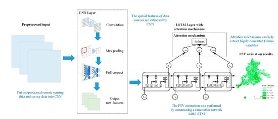
3.6. CNN-LSTM-Attention FSV Prediction Model

The FSV dataset based on multi-source remote sensing and survey data constructed in this study has the following characteristics: a large amount of spatial information and a time series based on survey time. The convolution kernel pooling operation unique to a convolutional neural network can extract the feature information of the data well, while LSTM has a strong memory and has a good effect on serialized data processing. Based on the advantages of the two neural network models, this study combines the two models to construct the FSV prediction model.

Using CNN to extract the potential features of FSV modeling variables can reduce the number of useless feature variables to compress the model training time and improve the prediction accuracy of FSV. The structure of the convolutional neural network is shown in Figure 5, including a convolution layer, a pooling layer for dimensionality reduction, and a fully connected layer. Firstly, all the feature variables extracted by preprocessing are normalized to ensure that the data scale input into CNN is the same. Then, the first feature fusion and extraction of variables are performed in the convolution layer through a 3 × 3 convolution kernel. Then, the maximum pooling method is used to extract the data twice through the pooling layer to reduce the amount of data required for FSV prediction. At the same time, the ReLU activation function is used after the pooling layer to enhance the ability of model learning. Finally, the secondary feature fusion and extracted data are re-formed into a one-dimensional array. The array is used as the input of the fully connected layer and is connected to the neurons of the upper structure to realize the transformation of the data dimension, while retaining the useful information of the data. Finally, the output of the new FSV prediction features is completed.

The long short-term memory network (LSTM) has great advantages in processing time series data, and it also has an excellent performance in establishing strong sequential and multivariate regression models. Adding an attention mechanism to LSTM can make the output layer of the network have higher discrimination to the output of the hidden layer, increase the weight of the strong correlation output, and improve the prediction accuracy of FSV. Therefore, this study constructs a FSV prediction model based on LSTM-Attention.

LSTM has a chain structure, which stores the state of neurons through the gate structure. The chain structure is shown in Figure 6. Each yellow box represents a neural network layer, which is composed of weight, bias, and the activation function; each green circle represents a pointwise operation; the arrows indicate the direction of the vector; the intersecting arrows represent the concatenation of vectors; and the bifurcated arrows represent the copy of the vector. LSTM has three inputs: cell state C_t−1 (blue circle), hidden layer state of the last moment h_t−1 (purple circle), and t time input vector x_t (blue circle), and the output has two: cell state at t time C_t and hidden layer state h_t. The information of the cell state C_t−1 is always transmitted on the line above. The hidden layer state h_t at time t and the input x_t will modify C_t appropriately and then pass it to the next moment. C_t−1 will participate in the calculation of the output h_t at time t. The information of the hidden layer state h_t−1 modifies the cell state through the gate structure of LSTM and participates in the calculation of the output. In general, the information of the cell state has been transmitted on the upper line, and the hidden layer state has been transmitted on the lower line. They interact with each other through the gate structure. In the three-gate structures, the results of 0~1 are calculated by the activation function σ to affect the proportion of the information access and abandonment of the previous neuron.

The gate structure increases the number of network iterations, and the error of the activation function can still be transmitted in reverse to avoid long-term dependence. At the same time, the output of the upper layer neurons is accepted by the three-gate structures of the forgetting gate, input gate, and output gate, and the effective information of the historical moment is selectively retained.

The forgetting gate calculation formula is as follows:

$$f_t=\sigma \left[w_f\left(h_{t-1},x_t\right)+b_f\right]$$

(4)

where w_f is the forgetting gate weight matrix and b_f is the forgetting gate bias.

The input gate calculation formula is as follows:

$$g_t=\sigma \left[w_g\left(h_{t-1},x_t\right)+b_g\right]$$

(5)

$${\tilde{P}}_t=\tanh \left[w_p\left(h_{t-1},x_t\right)+b_p\right]$$

(6)

$$P_t=f_t\cdot P_{t-1}+g_t\cdot {\tilde{P}}_t$$

(7)

where w_g is the input gate weight matrix, b_g is the input gate bias, ${\tilde{P}}_t$ is the input gate short-term state vector, w_p is the tanh layer weight matrix, b_p is the tanh layer bias, and P_t is the updated neuron state.

The output gate calculation formula is as follows:

$$y_t=\sigma \left[w_y\left(h_{t-1},x_t\right)+b_y\right]$$

(8)

$$h_t=y_t\cdot \tanh \left(P_t\right)$$

(9)

where y_t is the information to be output retained by the activation function σ, w_y is the output gate weight matrix, and b_y is the output gate bias.

For the FSV prediction model, the variables with a high correlation with FSV are found in many characteristic variables, and more weights are assigned to high correlation variables, which can improve the performance of model prediction. Therefore, the attention mechanism is introduced between the LSTM hidden layer and the output layer in this study.

Let the output data of the hidden layer be h_i, the weight value of the input data be a_i, and the final result calculated by the Attention mechanism be h*. The attention mechanism calculation formula is as follows:

$$h^{\ast }={\displaystyle \sum _{i=1}^t{a}_i{h}_i}$$

(10)

The correlation weight a_i of h_i and h* is calculated by the vector dot product scoring function. The greater the correlation is, the greater the result value of the scoring function is. The calculation formula is as follows:

$$s_i=f\left(h_i,h^{\ast }\right)=h_i\cdot h^{\ast }$$

(11)

After that, the weight value a_i is calculated by the weighted average of the Softmax function, and the sum of the weight values of all h_i is 1. The calculation formula is as follows:

$$a_i=softmax\left(s_i\right)$$

(12)

The structure between the hidden layer and the output layer of LSTM with an attention mechanism is shown in Figure 7.

Where x₀, x₁, x₂,…,x_t denotes the input characteristics of FSV; h₀, h₁, h₂,…,h_t represents the output value of the LSTM hidden layer; and a₀, a₁, a₂…,a_t represents the attention weight value of the attention mechanism to the output of the LSTM hidden layer. Calculate the weight a_i of the hidden layer output h_i to h* at each time. Then the weighted average calculation is carried out to obtain $V={\displaystyle \sum _{i=1}^t{a}_i{h}_i}$ and pass it to the softmax layer. The full connection calculation is carried out to obtain the output value of the output layer, that is, the FSV prediction value. The calculation formula is as follows:

$$y=softmax\left(W_{v}V+b_v\right)$$

(13)

where W_v is the weight matrix and b_v is the bias.

Finally, the model input of this study is the normalized data after Pearson correlation analysis and one-dimensional CNN preprocessing, which is input into the LSTM-Attention model [38]. The attention mechanism is introduced into the hidden layer to obtain the weighted average weight coefficient of the hidden layer output, and then the weight coefficient is multiplied by the output of the LSTM hidden layer to sum, and the result is input into the output layer of the LSTM for a full connection calculation. Finally, the output result is inversely normalized to obtain the prediction result of FSV [39]. The workflow of the entire model is shown in Figure 8.

3.7. Evaluating Indicator

In this study, all FSV estimation models were implemented in Python, and the training set and validation set were extracted through ten cross-validations of five replicates to evaluate the performance of the model and ensure the stability of all FSV estimation model results. The accuracy measurement of FSV in the test set includes four criteria, including the coefficient of determination (R²), mean square error (MSE), mean absolute error (MAE), and root mean square error (rMSE) between the observed and predicted FSV values. The formula is as follows:

$$R^2=\frac{{\displaystyle \sum _{i=1}^n{\left({\widehat{Y}}_i-\overline{Y}\right)}^2}}{{\displaystyle \sum _{i=1}^n{\left({\widehat{Y}}_i-\overline{Y}\right)}^2}}$$

(14)

$$MAE=\frac{1}{n}{\displaystyle \sum _{i=1}^n\left|{\widehat{y}}_i-y_i\right|}$$

(15)

$$MSE=\frac{1}{n}{\displaystyle \sum _{i=1}^n{\left({\widehat{y}}_i-y_i\right)}^2}$$

(16)

$$rMSE=\sqrt{\frac{1}{n}{\displaystyle \sum _{i=1}^n\left|{\widehat{y}}_i-y_i\right|}}$$

(17)

where n is the sample size, Y_i is the true value of the FSV of the i th sample, $\overline{y}$ is the mean value of the true value of the FSV of all samples, and ${\widehat{y}}_i$ is the FSV prediction value of the model for the ith sample.

The value of the coefficient of determination (R²) is between 0 and 1, which can reflect the correlation between the survey data of the forest stock volume and the predicted value of the model. The closer to 1, the higher the inversion accuracy. The average absolute error (MAE) is obtained by taking the mean of the absolute error, and its value is a natural number greater than or equal to 0, which can reflect the overall prediction error. The root mean square error (MSE) is opened to obtain the root mean square error (rMSE). The root mean square error is consistent with the dimension of the predicted value, which can reflect the degree of deviation between the predicted value and the true value. The smaller the value, the better the quality of the model and the higher the prediction accuracy.

4. Results and Analysis

All models and variable screening methods in this study are based on Python language and built with Tensorflow framework. The operating system is 64-bit Windows11, and the hardware configuration includes AMD Ryzen 7 5800 H 3.20 GHz (Advanced Micro Devices, Santa Clara, CA, USA), NVIDIA GeForce RTX 3060 (NVIDIA, Santa Clara, CA, USA), and 16.0 GB RAM.

4.1. Correlation Analysis and Variable Screening of Characteristic Variables

After preprocessing the remote sensing image data, this study uses the feature variables extracted from the LansSat8 image and SRTM data as potential predictors related to FSV. Through the Pearson correlation coefficient test in SPSS 22 software, the correlation analysis and screening of modeling factors were carried out for the obtained characteristic variables. The Pearson correlation coefficient can be used to describe the correlation between the characteristic variables and the ground real FSV data. In this study, the Pearson correlation coefficients between the survey FSV and all the extracted feature variables were calculated.

Among all 81 characteristic variables, 69 characteristic variables were significantly correlated with the stock volume when the confidence level (bilateral) was 0.01, and 5 feature variables were significantly correlated with FSV when the confidence level (bilateral) was 0.05. They are the B1 band of spectral features, the B5 difference feature of texture features, the homogeneity feature of B6 and B7 bands, and the third component of principal component features. Seven feature variables were not significantly correlated, namely, the B6 and B7 bands of spectral features, the correlation features of B1, B5, B6, and B7 bands of texture features, and the difference features of B2 bands.

In order to analyze the contribution of different feature variable types to stock estimation among the 69 retained feature variables, 6 different species feature variables were combined into 7 different datasets, as shown in

Table 4. Datasets and their characteristic factors.

Variable Sets	Types of Characteristic Variables
DataSet1	Vegetation index, Texture, PCA, Topography, Soil
DataSet2	Spectrum, Texture, PCA, Topography, Soil
DataSet3	Spectrum, Vegetation index, PCA, Topography, Soil
DataSet4	Spectrum, Vegetation index, Texture, Topography, Soil
DataSet5	Spectrum, Vegetation index, Texture, PCA, Soil
DataSet6	Spectrum, Vegetation index, Texture, PCA, topography
DataSet7	Spectrum, Vegetation index, Texture, PCA, Topography, Soil

, which are: (1) datasets including the vegetation index feature, texture feature, principal component feature, topographic feature, and second-class survey feature as independent variables; (2) datasets containing spectral features, texture features, principal component features, topographic features, and second-class survey features as independent variables; (3) datasets containing spectral features, vegetation index features, principal component features, topographic features, and second-class survey features as independent variables; (4) datasets containing spectral features, vegetation index features, texture features, terrain features, and second-class survey features as independent variables; (5) datasets containing spectral features, vegetation index features, texture features, principal component features, and second-class survey features as independent variables; (6) datasets containing spectral features, vegetation index features, texture features, principal component features, and topographic features as independent variables; (7) contains datasets that retain all feature variables as independent variables.

4.2. Evaluation of Contribution Degree of Characteristic Variables

The CNN-LSTM-Attention model is used to test the above six datasets, respectively. The estimated accumulation of each dataset on the model is shown in

Table 5. The evaluation indexes of each dataset.

Variable Sets	R2	MAE	MSE	RMSE
Dataset1	0.6481	25.2271	1625.2519	40.3144
Dataset2	0.6208	25.5053	1751.4848	41.8507
Dataset3	0.7311	22.0368	1241.9801	35.2417
Dataset4	0.8299	17.4181	785.5955	28.0284
Dataset5	0.7633	21.5353	1093.2510	33.0643
Dataset6	0.8519	16.7629	683.8263	26.1501
Dataset7	0.8544	15.0753	672.3985	25.9306

and Figure 9.

According to the test results of different kinds of feature factor combinations shown in Figure 10, it can be seen that the highest coefficient of determination(R²) of dataset7 with the most types of characteristic variables is 0.8544; the second is dataset6 that lacks the information of soil characteristics. The coefficient of determination is 0.8519, and the root mean square error between the two datasets is only within 0.3 m³/ha, which may be due to the fact that the soil in the study area is generally not very different, which weakens the influence of the soil environment on vegetation growth. Among all kinds of characteristic variables, the original spectral characteristics of remote sensing images and the vegetation index characteristics that can directly reflect the vegetation growth status have the greatest impact on the estimation of volume. In the dataset lacking spectral characteristics and vegetation index characteristics, the root mean square error of the model is larger than that of other datasets, reaching 40.3144 m³/ha and 41.8507 m³/ha, respectively. The coefficient of determination(R²) decreased to 0.6481 and 0.6208. It can be seen that spectral data is the characteristic factor that can directly reflect the growth status of ground vegetation, and has a high contribution in the characteristic variables of volume estimation.

4.3. Comparison of FSV Prediction Results of Different Models

Based on the dataset composed of feature variables selected in the previous section, MLR, RF, LSTM, and CNN-LSTM-Attention models were used to predict the FSV of Baishanzu Forest Park. The overall FSV prediction results of the four models of MLR, RF, BP neural network, and CNN-LSTM-Attention on the test set after training on the dataset are shown in the Figure 11. The green area indicates the sample with a difference between the predicted FSV and the actual FSV less than 50 m³/ha. The blue area represents the sample with a difference of more than 50 m³/ha between the predicted FSV and the actual FSV.

Table 6. Evaluation indexes of different models.

Models	R2	MAE	MSE	RMSE
MLR	0.4071	35.9544	2738.3639	52.3293
RF	0.4754	33.1304	2422.7285	49.2212
BP	0.5518	30.6080	2070.1305	45.4986
CNN-LSTM-Attention	0.8519	16.7629	683.8263	26.1501

shows the results of four different models using a combination of feature variables based on correlation analysis filtered Landsat 8 images, SRTM digital elevation data, and survey data. The CNN-LSTM-Attention model showed the highest inversion accuracy, and both rMSE and MAE values were minimized (R² = 0.8519, rMSE = 26.1501 m³/ha, MAE = 16.7629 m³/ha). The inversion accuracy of BP model without parameter optimization decreases, the Coefficient of Determination (R²) is 0.5518. Compared with the neural network model, the accuracy of RF and MLR models is greatly decreased, and their Coefficient of Determination (R²) are less than 0.5, which can not be applied to practical tasks.

4.4. FSV Mapping of the Study Area

Based on the four different FSV estimation models, we estimate the FSV for the entire study area. The results are shown in

Table 7. FSV mapping results of different models.

Models	Minimum FSV (m3/ha)	Maximum FSV (m3/ha)	Total FSV (m3)	Accurate (%)
MLR	9.76	396.85	6,331,850.47	66.74
RF	4.13	359.17	3,017,532.16	71.40
BP	1.27	724.68	5,798,483.77	72.88
CNN-LSTM-Attention	4.83	402.38	5,066,562.23	83.41
Survey data	6.95	414.6	4,226,019.56	1

. After removing the non-forest samples, the model estimates that the minimum FSV of the Baishanzu Forest Park is 4.83 m³/ha, and the maximum is 402.38 m³/ha. The minimum FSV of the actual stand was 6.95 m³/ha, and the maximum was 414.6 m³/ha. The estimated total amount of FSV is 4,226,019.56 m³. According to the forest survey data, the total amount of FSV in Baishanzu Forest Park is 5,066,562.23 m³. Therefore, the accuracy of CNN-LSTM-Attention in predicting the FSV in Baishanzu Forest Park reached 83.41%.

It can be seen that the CNN-LSTM-Attention model has the highest accuracy for FSV estimation in the whole study area. So, based on the CNN-LSTM-Attention model, we drew the FSV of Baishanzu Forest Park, as shown in Figure 12, where (a) is the FSV drawn based on forest survey data and (b) is the FSV drawn according to the model estimation results.

By comparing the DEM data of the study area, it can be seen that the high FSV area in the study area is mainly concentrated in the low altitude area, mainly 600~800 m, and the vegetation in this range is mainly evergreen broad-leaved forest. As the altitude increases, the temperature gradually decreases, and the environmental climate is no longer suitable for the growth of most vegetation, so the FSV gradually decreases. In the area above the altitude of 1200 m, vegetation is mainly coniferous forest and its distribution is relatively sparse.

5. Conclusions and Discussion

This paper takes Baishanzu Forest Park in China as the research object, selects Landsat 8 and SRTM as the remote sensing data sources, and takes the spectrum, vegetation index, texture, PCA, topography, and soil from the two remote sensing data and survey data as the modeling factors. Firstly, the Pearson correlation analysis method is used to retain the factors with a high correlation with FSV and discard the low correlation and collinearity factors. Secondly, seven datasets were constructed based on the retained factors to evaluate the importance of different types of factors to FSV estimation. Finally, the CNN-LSTM-Attention model is proposed to estimate the FSV, and the accuracy of prediction results is compared with the MLR, RF, and BP models widely used at present. The experimental results show that the CNN-LSTM-Attention model, which combines the advantages of the CNN layer to extract deep features and LSTM to solve long-term dependence problems, is superior to other existing models in both prediction accuracy and prediction time.

However, there are still some aspects that need further study and improvement. Although the proposed method combined with convolution can fuse input features to make the network use remote sensing variables more effectively, the performance of the network under different hyperparameters still varies with the increase in the number of input variables, which indicates that the targeted adjustment of network parameters according to the type of input characteristic variables can further improve the prediction accuracy. In addition, the parameters used in this experiment may not be applicable to other datasets, which indicates that the further study of spectral features expressed by forest remote sensing images in different regions is needed to improve the robustness of the network.

With the continuous improvement of computer computing power, the regression model based on neural network can not only be applied to other problems other than FSV estimation, but also can be built in small servers such as home servers due to the lightweight of the model. Therefore, it is necessary for future research to combine more machine learning algorithms and innovative machine learning methods. In addition, the main method to predict FSV by combining multi-source remote sensing data is to combine active remote sensing data with single optical remote sensing data. However, compared to optical remote sensing data, active remote sensing data are relatively expensive and difficult to obtain. As a result, the limitation of this study is that only Landsat and SRTM passive remote sensing data are combined. In future experiments, more different bands of heterogeneous remote sensing data can be attempted for image fusion, which may obtain better FSV prediction results.

References

1. Seidl, R.; Schelhaas, M.J.; Rammer, W.; Verkerk, P.J. Increasing forest disturbances in Europe and their impact on carbon storage. Nat. Clim. Chang. 2014, 4, 806–810. [Google Scholar] [CrossRef] [PubMed]
2. Pugh, T.A.M.; Lindeskog, M.; Smith, B.; Poulter, B.; Arneth, A.; Haverd, V.; Calle, L. Role of forest regrowth in global carbon sink dynamics. Proc. Natl. Acad. Sci. USA 2019, 116, 4382–4387. [Google Scholar] [CrossRef] [PubMed]
3. Hu, Y.; Xu, X.; Wu, F.; Sun, Z.; Xia, H.; Meng, Q.; Huang, W.; Zhou, H.; Gao, J.; Li, W.; et al. Estimating forest stock volume in Hunan Province, China, by integrating in situ plot data, Sentinel-2 images, and linear and machine learning regression models. Remote Sens. 2020, 12, 186. [Google Scholar] [CrossRef]
4. Le Toan, T.; Quegan, S.; Davidson, M.W.J.; Balzter, H.; Paillou, P.; Papathanassiou, K.; Plummer, S.; Rocca, F.; Saatchi, S.; Shugart, H.; et al. The BIOMASS mission: Maping global forest biomass to better understand the terrestrial carbon cycle. Remote Sens. Environ. 2011, 115, 2850–2860. [Google Scholar] [CrossRef]
5. Xu, X.; Lin, H.; Liu, Z.; Ye, Z.; Li, X.; Long, J. A combined strategy of improved variable selection and ensemble algorithm to map the growing stem volume of planted coniferous forest. Remote Sens. 2021, 13, 4631. [Google Scholar] [CrossRef]
6. Fang, G.; Fang, L.; Yang, L.; Wu, D. Comparison of Variable Selection Methods among Dominant Tree Species in Different Regions on Forest Stock Volume Estimation. Forests 2022, 13, 787. [Google Scholar] [CrossRef]
7. Astola, H.; Häme, T.; Sirro, L.; Molinier, M.; Kilpi, J. Comparison of Sentinel-2 and Landsat 8 imagery for forest variable prediction in boreal region. Remote Sens. Environ. 2019, 223, 257–273. [Google Scholar] [CrossRef]
8. Jiang, F.; Kutia, M.; Ma, K.; Chen, S.; Long, J.; Sun, H. Estimating the aboveground biomass of coniferous forest in Northeast China using spectral variables, land surface temperature and soil moisture. Sci. Total Environ. 2021, 785, 147335. [Google Scholar] [CrossRef]
9. Fassnacht, F.; Hartig, F.; Latifi, H.; Berger, C.; Hernández, J.; Corvalán, P.; Koch, B. Importance of sample size, data type and prediction method for remote sensing-based estimations of aboveground forest biomass. Remote Sens. Environ. 2014, 154, 102–114. [Google Scholar] [CrossRef]
10. Lu, D. The potential and challenge of remote sensing-based biomass estimation. Int. J. Remote Sens. 2006, 27, 1297–1328. [Google Scholar] [CrossRef]
11. Tanaka, S.; Takahashi, T.; Nishizono, T.; Kitahara, F.; Saito, H.; Iehara, T.; Kodani, E.; Awaya, Y. Stand volume estimation using the k-NN technique combined with forest inventory data, satellite image data and additional feature variables. Remote Sens. 2014, 7, 378–394. [Google Scholar] [CrossRef]
12. Puliti, S.; Saarela, S.; Gobakken, T.; Ståhl, G.; Næsset, E. Combining UAV and Sentinel-2 auxiliary data for forest growing stock volume estimation through hierarchical model-based inference. Remote Sens. Environ. 2018, 204, 485–497. [Google Scholar] [CrossRef]
13. Sánchez-Ruiz, S.; Moreno-Martínez, Á.; Izquierdo-Verdiguier, E.; Chiesi, M.; Maselli, F.; Gilabert, M.A. Growing stock volume from multi-temporal landsat imagery through google earth engine. Int. J. Appl. Earth Obs. Geoinf. 2019, 83, 101913. [Google Scholar] [CrossRef]
14. Chrysafis, I.; Mallinis, G.; Tsakiri, M.; Patias, P. Evaluation of single-date and multi-seasonal spatial and spectral information of Sentinel-2 imagery to assess growing stock volume of a Mediterranean forest. Int. J. Appl. Earth Obs. Geoinf. 2019, 77, 1–14. [Google Scholar] [CrossRef]
15. Sun, H.; Wang, Q.; Wang, G.; Lin, H.; Luo, P.; Li, J.; Zeng, S.; Xu, X.; Ren, L. Optimizing kNN for mapping vegetation cover of arid and semi-arid areas using landsat images. Remote Sens. 2018, 10, 1248. [Google Scholar] [CrossRef]
16. Sichangi, A.W.; Makokha, G.O. Monitoring water depth, surface area and volume changes in Lake Victoria: Integrating the bathymetry map and remote sensing data during 1993–2016. Model. Earth Syst. Environ. 2017, 3, 533–538. [Google Scholar] [CrossRef]
17. Dube, T.; Mutanga, O.; Abdel-Rahman, E.M.; Ismail, R.; Slotow, R. Predicting Eucalyptus spp. stand volume in Zululand, South Africa: An analysis using a stochastic gradient boosting regression ensemble with multi-source data sets. Int. J. Remote Sens. 2015, 36, 3751–3772. [Google Scholar] [CrossRef]
18. Mura, M.; Bottalico, F.; Giannetti, F.; Bertani, R.; Giannini, R.; Mancini, M.; Orlandini, S.; Travaglini, D.; Chirici, G. Exploiting the capabilities of the Sentinel-2 multi spectral instrument for predicting growing stock volume in forest ecosystems. Int. J. Appl. Earth Obs. Geoinf. 2018, 66, 126–134. [Google Scholar] [CrossRef]
19. Soomro, B.N.; Xiao, L.; Huang, L.; Soomro, S.H.; Molaei, M. Bilayer elastic net regression model for supervised spectral-spatial hyperspectral image classification. IEEE J. Sel. Top. Appl. Earth Obs. Remote Sens. 2016, 9, 4102–4116. [Google Scholar] [CrossRef]
20. Marino, E.; Ranz, P.; Tomé, J.L.; Noriega, M.; Esteban, J.; Madrigal, J. Generation of high-resolution fuel model maps from discrete airborne laser scanner and Landsat-8 OLI: A low-cost and highly updated methodology for large areas. Remote Sens. Environ. 2016, 187, 267–280. [Google Scholar] [CrossRef]
21. Gasparini, P.; Di Cosmo, L.; Rizzo, M.; Giuliani, D. A stand-level model derived from National Forest Inventory data to predict periodic annual volume increment of forests in Italy. J. For. Res. 2017, 22, 209–217. [Google Scholar]
22. Cao, L.; She, G.H. Inversion of Forest Stand Characteristics Using Small-Footprint Full-Waveform Airborne Li DAR in a Subtropical Forest. Sci. Silvae Sin. 2015, 51, 81–92. [Google Scholar]
23. Fu, L.; Liu, Q.; Sun, H.; Wang, Q.; Li, Z.; Chen, E.; Pang, Y.; Song, X.; Wang, G. Development of a system of compatible individual tree diameter and aboveground biomass prediction models using error-in-variable regression and airborne LiDAR data. Remote Sens. 2018, 10, 325. [Google Scholar] [CrossRef]
24. Sheridan, R.D.; Popescu, S.C.; Gatziolis, D.; Morgan, C.L.S.; Ku, N.-W. Modeling forest aboveground biomass and volume using airborne LiDAR metrics and forest inventory and analysis data in the Pacific Northwest. Remote Sens. 2014, 7, 229–255. [Google Scholar] [CrossRef]
25. Sefercik, U.G.; Yastikli, N.; Dana, I. DEM extraction in urban areas using high-resolution TerraSAR-X imagery. J. Indian Soc. Remote Sens. 2014, 42, 279–290. [Google Scholar] [CrossRef]
26. Varvia, P.; Lähivaara, T.; Maltamo, M.; Packalen, P.; Tokola, T.; Seppänen, A. Uncertainty quantification in ALS-based species-specific growing stock volume estimation. IEEE Trans. Geosci. Remote Sens. 2016, 55, 1671–1681. [Google Scholar] [CrossRef]
27. Dos Reis, A.A.; Franklin, S.E.; de Mello, J.M.; Junior, F.W.A. Volume estimation in a Eucalyptus plantation using multi-source remote sensing and digital terrain data: A case study in Minas Gerais State, Brazil. Int. J. Remote Sens. 2019, 40, 2683–2702. [Google Scholar] [CrossRef]
28. Xiao, W.; Vallet, B.; Brédif, M.; Paparoditis, N. Street environment change detection from mobile laser scanning point clouds. ISPRS J. Photogramm. Remote Sens. 2015, 107, 38–49. [Google Scholar] [CrossRef]
29. Silva, C.A.; Hudak, A.T.; Vierling, L.A.; Klauberg, C.; Garcia, M.; Ferraz, A.; Keller, M.; Eitel, J.; Saatchi, S. Impacts of airborne lidar pulse density on estimating biomass stocks and changes in a selectively logged tropical forest. Remote Sens. 2017, 9, 1068. [Google Scholar] [CrossRef]
30. Lu, D.; Chen, Q.; Wang, G.; Liu, L.; Li, G.; Moran, E. A survey of remote sensing-based aboveground biomass estimation methods in forest ecosystems. Int. J. Digit. Earth 2016, 9, 63–105. [Google Scholar] [CrossRef]
31. Zhang, Y.; Ma, J.; Liang, S.; Li, X.; Li, M. An evaluation of eight machine learning regression algorithms for forest aboveground biomass estimation from multiple satellite data products. Remote Sens. 2020, 12, 4015. [Google Scholar] [CrossRef]
32. Pham, T.D.; Yokoya, N.; Xia, J.; Ha, N.T.; Le, N.N.; Nguyen, T.T.T.; Dao, T.H.; Vu, T.T.P.; Pham, T.D.; Takeuchi, W. Comparison of machine learning methods for estimating mangrove above-ground biomass using multiple source remote sensing data in the red river delta biosphere reserve, Vietnam. Remote Sens. 2020, 12, 1334. [Google Scholar] [CrossRef]
33. Gao, Y.; Lu, D.; Li, G.; Wang, G.; Chen, Q.; Liu, L.; Li, D. Comparative analysis of modeling algorithms for forest aboveground biomass estimation in a subtropical region. Remote Sens. 2018, 10, 627. [Google Scholar] [CrossRef]
34. Haapanen, R.; Tuominen, S. Data combination and feature selection for multi-source forest inventory. Photogramm. Eng. Remote Sens. 2008, 74, 869–880. [Google Scholar] [CrossRef]
35. Oliveira, L.Z.; Vibrans, A.C. Evaluating Trade-Offs between Using Regional and Site-Specific Allometric Models to Predict Growing Stock Volume of Subtropical Atlantic Forests. For. Sci. 2022, 68, 365–375. [Google Scholar] [CrossRef]
36. Torre-Tojal, L.; Bastarrika, A.; Boyano, A.; Lopez-Guede, J.M.; Graña, M. Above-ground biomass estimation from LiDAR data using random forest algorithms. J. Comput. Sci. 2022, 58, 101517. [Google Scholar] [CrossRef]
37. Huete, A.; Justice, C.; Liu, H. Development of vegetation and soil indices for MODIS-EOS. Remote Sens. Environ. 1994, 49, 224–234. [Google Scholar] [CrossRef]
38. Padilla-Martínez, J.R.; Paul, C.; Husmann, K.; Corral-Rivas, J.J.; von Gadow, K. Grouping tree species to estimate basal area increment models in temperate multispecies forests in Durango, Mexico. For. Ecosyst. 2023, 11, 100158. [Google Scholar] [CrossRef]
39. Zhou, Y.; Feng, Z. Estimation of Forest Stock Volume Using Sentinel-2 MSI, Landsat 8 OLI Imagery and Forest Inventory Data. Forests 2023, 14, 1345. [Google Scholar] [CrossRef]
Figure 1. Overview of study area.
Remotesensing 16 00324 g001
Figure 2. Nine vegetation index grayscale in the study area: (a) BVI; (b) DVI; (c) EVI; (d) GVI; (e) NDVI; (f) PVI; (g) RVI; (h) TVI; (i) WVI.
Remotesensing 16 00324 g002
Figure 3. Eigenvalues of each principal component.
Remotesensing 16 00324 g003
Figure 4. Topographic factors in the study area: (a) DEM and (b) slope.
Remotesensing 16 00324 g004
Figure 5. CNN structure diagram.
Remotesensing 16 00324 g005
Figure 6. Expansion diagram of LSTM structure: (a) chain structure of LSTM; (b) the vector direction inside the LSTM’s three-gate structure.
Remotesensing 16 00324 g006
Figure 7. LSTM model with attention mechanism.
Remotesensing 16 00324 g007
Figure 8. CNN-LSTM-Attention FSV estimation model.
Remotesensing 16 00324 g008
Figure 9. Estimated result of each dataset: (a) Dataset1; (b) Dataset2; (c) Dataset3; (d) Dataset4; (e) Dataset5; (f) Dataset6; (g) Dataset7.
Remotesensing 16 00324 g009aRemotesensing 16 00324 g009b
Figure 10. MSE of each dataset: (a) Dataset1; (b) Dataset2; (c) Dataset3; (d) Dataset4; (e) Dataset5; (f) Dataset6; (g) Dataset7.
Remotesensing 16 00324 g010aRemotesensing 16 00324 g010b
Figure 11. FSV prediction results of different models: (a) MLR; (b) RF; (c) BP; (d) CNN-LSTM-Attention.
Remotesensing 16 00324 g011aRemotesensing 16 00324 g011b
Figure 12. FSV inversion results: (a) real FSV and (b) predicted FSV.
Remotesensing 16 00324 g012