
A Case Study of Wave–Wave Interaction South to Dongsha Island in the South China Sea


1
College of Marine Technology and Environment, Dalian Ocean University, Dalian 116023, China
2
Frontier Science Center for Deep Ocean Multispheres and Earth System (FDOMES) and Physical Oceanography Laboratory, Ocean University of China, Qingdao 266100, China
3
School of Mathematical Sciences, Ocean University of China, Qingdao 266100, China
*
Author to whom correspondence should be addressed.
Remote Sens. 2024, 16(2), 337; https://doi.org/10.3390/rs16020337
Submission received: 22 November 2023
/
Revised: 29 December 2023
/
Accepted: 8 January 2024
/
Published: 15 January 2024
(This article belongs to the Special Issue Advances in Oceanic Dynamics by SAR and Numeric Model in Tropical Cyclone)
Abstract
:In a SAR image acquired by the ERS-2 satellite, crossed “X-shape” internal solitary waves (ISWs) south to Dongsha Island are found to be a wave–wave interaction composed of five solitons: two head waves, two tail waves, and the overlapped part. To explain this remote sensing phenomenon, based on a high-resolution three-dimensional MIT general circulation model (MITgcm) using realistic topography and tidal forcing, the “X-shape” internal waves are reproduced at the same location. The development processes of the waves indicate that the “X-shape” ISWs are two waves diffracted from one internal wave southeast to Dongsha Island. During the propagation, the amplitude of their overlapped part of the “X-shape” ISWs becomes significantly larger than the sum of the amplitudes of both head waves, which proves that nonlinear wave–wave interaction has occurred. Based on wave–wave interaction theory, the theoretical maximum value of the amplitude of the overlapped part at the initial moment is calculated as 14.12 m, which is in good agreement with the model results of 14 m. Meanwhile, the variation of the theoretical amplitude of the overlapped part is basically consistent with that of the modeled one, confirming the occurrence of the wave–wave interaction. Besides, when the waves propagate over varying water depths, the type of the wave–wave interaction can change rather than being fixed from the start.
1. Introduction
The ocean is a key component of the earth’s climate system, and mixing processes are critical in determining its distribution of salt and heat [1]. As an important marine dynamic process, internal waves (IWs) are one of the major sources of mixing in the ocean. It has a significant influence on mass transportation in the ocean [2]. In terms of energy in the ocean, the energy transfer and exchange between marine phenomena occur on different temporal and spatial scales. The IW, a mesoscale and sub-mesoscale dynamic phenomenon, plays an important role in the whole energy cascade of the ocean. However, it is usually difficult to monitor IWs for long-term and large-area observations by conventional observation methods. Therefore, satellite remote sensing has gradually become one of the most important ways to study IWs. Compared with visible light and infrared sensors, SAR (synthetic aperture radar) has more advantages for observing IWs because it usually has high resolution and is not affected by clouds or bad weather.
Wave–wave interaction may occur when two IWs meet. Under certain conditions, a new IW will be generated in the interaction zone. The amplitude of the newly generated IW can be up to four times that of the pre-interacting IWs [3,4]. During the whole interaction process, the shape, amplitude, and propagation velocity of the pre-interacting IWs may change substantially. Therefore, wave–wave interaction not only has an important impact on the distribution of salt and heat fields and the dynamic structure of the ocean but also greatly enhances the destructive power of the ocean engineering structures and the threat to the safety of underwater vehicles. It has become a frontier topic in the fields of nonlinear science, ocean engineering, and even ecological environment in recent years [5,6,7,8,9]. Figuring out the evolution of physical characteristics of internal waves such as shape, amplitude, and energy in the process of wave–wave interaction can help us better understand the propagation of the internal waves and also steepen our understanding of energy cascades at middle and small scales in the ocean. The wave–wave interaction theory was first proposed by Miles [3,4]. The interaction of two surface solitary waves of equal amplitude was studied based on the Korteweg–de Vries (KdV) equation [10] and Boussinesq-type equations [11]. It was found that the change in the amplitude or the angle between the two interacting waves would lead to different forms and transmission characteristics of the waves. In particular, when the interacting angles met certain conditions, a new wave with a larger amplitude arose from the interaction zone, which was called the Mach stem. This theory was confirmed by laboratory experiments [12], numerical simulations [13], and theoretical analyses [14]. Nevertheless, it is relatively recent that this theory was extended to the conditions of small-but-finite angles, as the Kadomtsev–Petviashvili (KP) equation was introduced in [15]. The KP equation can be regarded as a two-dimensional version of the KdV equation, although formally only for weak transverse effects. It was first proposed by Kadomtsev and Petviashvili [16]. However, the theory of wave–wave interaction has seldom been applied to the internal solitary waves in realistic oceans until now. Some studies on the wave–wave interaction are based on the KP equation [17,18,19] to evaluate how effective the theory is when applied to the IWs in the ocean. The interactions of IWs under realistic oceanic conditions are a little bit different from those of surface solitary waves because there are more factors at play. The main influencing factors include strong linearity [20], topography, and Earth’s rotation [21]. Shimizu et al. [22] take these factors into account and add them to the KP equation to explore how much these terms affect. The results show that the solutions to the modified KP equation are almost consistent with those of the traditional Miles theory.
For in-situ observations of the wave–wave interaction, it is difficult to satisfy the requirements for both horizontal and temporal coverage and resolution for underwater measurements. Therefore, the in-situ measurement-based study of the wave–wave interaction has been very limited up to now. For instance, Wang and Pawlowicz [23] conducted measurements on the wave–wave interactions of near-surface internal waves in the Strait of Georgia, but the results are not quite consistent with the wave–wave interaction theory.
Another way to study the wave–wave interaction is the numerical modeling approach. However, the numerical studies targeted at wave–wave interactions are also few so far. Shimizu et al. [22] conducted a series of numerical sensitivity simulations to investigate the influence of factors such as topography on the wave–wave interaction in the Andaman Sea. The results are mentioned above.
The northern South China Sea is one of the oceans with the most frequent IWs in the world. Previous studies [24,25,26,27,28] have shown that IWs in the northern South China Sea originate from the Luzon Strait. These IWs propagate westward, pass through the deep basin, shoal on the shelf near Dongsha Island, and finally dissipate. The seabed topographies have been shown to have significant impacts on water waves [29,30]. The topography near Dongsha Island is complicated with many small seamounts and ridges, which can diffract the westward propagating IWs into two branch waves [31]. Then the south branch and north branch waves may meet and cross when they propagate further westward after the diffraction. In the propagation process, IWs can cause local upwelling and downwelling, which affect the distribution of the sea surface flow field and then change the distribution of micro-scale surface waves, resulting in changes in sea surface roughness. In this way, remote sensing satellites will receive reflected signals of different intensities, forming bright and dark stripes on the satellite image [32]. Therefore, remote sensing satellites, especially SAR satellites, can be used to detect the spatial position of internal waves and the characteristics of wave crests. SAR images have shown a lot of crossed crest lines of IWs near Dongsha Island, indicating that wave–wave interaction may happen [33]. Several papers [31,34,35] have studied wave–wave interaction near Dongsha Island using SAR data; however, explanations of the SAR-based wave–wave interaction in the northern South China Sea are still lacking.
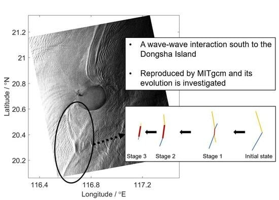
In a SAR image obtained by ERS-2 (Figure 1a), crossed “X-shape” ISWs south to Dongsha Island are found. The waves are composed of five solitons: two head waves, two tail waves, and the overlapped part. The overlapped part is a stem-like wave, and its backscattering coefficient is larger than those of other solitons (two head waves and two tail waves), which suggests that a wave–wave interaction occurs here.
This satellite image reveals perfect evidence of the wave–wave interaction but cannot provide information on the interior structure of the IWs and its associated evolution processes. Three interesting questions arise here: First, how does the wave–wave interaction in Figure 1 forms? Second, how do the shape and characteristic parameters, such as the amplitude of the internal waves, change during the wave–wave interaction? Third, what about the corresponding energy change during the wave–wave interaction? To answer these questions, a numerical model and the wave–wave interaction theory will be used in this paper.
The paper is organized as follows: Section 2 introduces the numerical model configuration and validation. In Section 3, the wave–wave interaction in the SAR image is reproduced by using the ocean model, and the physical parameters such as shape, amplitude, and energy flux in the whole evolution process are calculated and described by combining the wave–wave interaction theory. Section 4 makes detailed comparisons between the theory and model results, analyzes the evolution characteristics of this wave–wave interaction, and draws conclusions.
2. Model Setup and Validation
2.1. Model Setup
The MITgcm (Massachusetts Institute of Technology General Circulation Model) is able to simulate multi-scale ocean processes, including internal waves, and will be applied in this research. The MITgcm uses finite volume methods and orthogonal curvilinear coordinates horizontally. The model domain (115.5°E–122.4°E and 17.7°N–22.4°N) is shown in Figure 1b. Since the propagation directions of IWs in the northern South China Sea are mainly northwestward and westward [24], and this paper focuses on the area around Dongsha Island, the horizontal resolution is set to 150 m (west to 117.5°E)/300 m (east to 117.5°E) in the zonal direction and 400 m in the meridional direction. Besides, a transition zone of 15 grid points is settled along 117.5°E. In the transition zone, the zonal width difference between adjacent grids is 10 m, which gradually decreases from 300 m in the west to 150 m in the east. There are 150 model layers in vertical, with higher resolution in the upper ocean (1 m near the surface layer) to better characterize the IWs and coarser resolution in the deeper ocean (200 m near the bottom layer) to save on calculation costs. Topographic data from the GEBCO dataset (General Bathymetric Chart of the Oceans, https://www.gebco.net/data_and-_products/historical_data_sets/#gebco_2014, accessed on 12 June 2022) is interpolated linearly to match the girds. The minimum water depth is set at 1 m, while the maximum water depth is 5160 m.
Initial conditions are horizontally uniform stratification and no flow. The salinity and temperature data are from the climatological data of June from the WOA dataset (World Ocean Atlas, https://www.nodc.noaa.gov/OC5/woa13/, accessed on 5 December 2019) and input into the model after being horizontally averaged in the study area. Boundary conditions are no stress at the surface, no slip at the bottom, and no buoyancy flux through the surface or the bottom. At four open boundaries, eight barotropic tides (K1, O1, P1, Q1, M2, S2, K2, and N2) forced the model from 20 to 25 June 2005. The amplitudes and phases of these tides are acquired from the TPXO8-atlas dataset (https://www.tpxo.net/global/tpxo8-atlas, accessed on 18 May 2021) [37]. Meanwhile, a sponge boundary treatment [38] with a width of 50 grid points is adapted to avoid the reflection of IWs. The KPP scheme, whose mixing below the surface mixed layer is represented by a background viscosity/diffusivity (assumed constants) and a viscosity/diffusivity based on shear instability, is used. For the horizontal mixing scheme, the Leith scheme [39] is used to provide enough viscous dissipation to damp divergence and vorticity at the grid scale. The time interval for output data is 10 min.
2.2. Model Validation
2.2.1. Comparison with In-Situ Measurements
In the WISE/VANS project [36], the tidal current velocity at mooring L1 (20.5897°N and 121.9187°E, shown as the red circle in Figure 1) is observed by using upward-looking 300 kHz ADCP mounted in a cage 4 m off the bottom-sampled 4 m bins every 15 min from 25 April to 28 October 2005. The instrument depth is 455 m. The measured depth range of velocity is 380 m to 450 m, so we select the model data from the same depth range to make the comparisons. The vertically averaged values of the measurements and model results from 17 to 30 June 2005 are shown in Figure 2a. It can be seen that even though there are some differences between the maximum values of the model results and the measured results from 21 to 24 June, the overall trend of variation of the model results is consistent with that of the measured results, so we think that the model results are valid and can be used for further analysis.
2.2.2. Comparison with SAR Image
Using SAR satellite images, the location of IWs and the distribution of wave crests can be tracked. Figure 2b shows a SAR snapshot, which includes two IWs west of the Luzon Strait. One is around 118.1°E and has an arc shape with tail waves, while the other is around 117.2°E and is a soliton. For the model results, we apply a method similar to Zhang et al. [38] to locate the IWs. We calculate the sea surface height gradient (SSHG):
where ζ (x, y) is the height of the sea surface at a certain moment. In our model, the x and y, respectively, indicate the zonal and meridional directions. Figure 2c shows the SSHG at 39 h of model time (hereafter “model time” is omitted). There are two sets of IWs west of the Luzon Strait, and we name them W1 and W2. W1 is a wave train and located around 118.2°E, while W2 is a soliton and located at about 117.3°E. The forms of both waves are slightly different from those in the SAR image. The tail waves of W1 are weaker and more concentrated. The northern part of W2 (north of about 21.5°N) is more westerly, and the SSHG decreases rapidly to the north of 21.8°N, while the white stripes in SAR images can still be distinguished to the north of 22.0°N. Overall, the simulated results are consistent with the SAR sensing results.
3. Results
3.1. Model-Produced Amplitudes of the Internal Waves
Based on the model results, to describe the propagation processes of IWs near Dongsha Island, the SSHG is calculated at each moment. It is found that the IWs at 52 h 20 min (Figure 3a) are closest to those from the SAR image in Figure 1a. Although their positions are not exactly identical, their main characteristics are the same. First, both have stem-like waves at the overlapped part and whose values (backscatter intensity in the SAR image and SSHG in the model results) are larger than rest solitons. Second, the values of the head waves are larger than those of the tail waves. These two arguments suggest that wave–wave interaction has occurred here. Therefore, it is necessary to calculate the amplitudes of each soliton, that is, two head waves, two tail waves, and the interaction zone, to see how the interaction is. As the model results include salinity, temperature, and current velocity, we follow the method proposed by Buijsman et al. [40] to calculate the waves’ amplitudes. The detailed decomposition and solution are given in Appendix A, and a brief introduction is given below. An IW can be viewed as consisting of a series of different modes and partial tides. From the point of view of a mathematical equation, the problem of internal wave vertical structure can be reduced to the Sturm-Liouville eigenvalue problem [41]. For an IW of a certain frequency, it has the characteristics of stratification in the whole water depth range, so we can use the temperature, salinity, and velocity data at different layers in our model to calculate the different modes of the IW [42]. By solving the Sturm-Liouville equation, the coefficients of each mode and partial tides can be determined, and thus the amplitudes are acquired for any wave of a specific mode.
The M2 tide is dominant near Dongsha Island, and here, we use the M2, M4, M6, and M8 frequencies. Meanwhile, we use the first 10 modes to calculate the isopycnal displacement term. Figure 3b shows the results of the first three vertical modes at section IZ at 52 h and 20 min. Similarly, we calculate the isopycnal displacement term at sections H1, H2, T1, and T2, as listed in Table 1. Note that the water depth is acquired at the midpoint of the cross-section.
It can be seen that the amplitude of the interaction zone (section IZ) is larger than the sum of the amplitudes of the two head waves (sections H1 and H2), which indicates that the two waves do have nonlinear interaction at the overlapped part, which forms a stem-like wave.
3.2. Spatial and Temporal Variation of the Wave–Wave Interaction
As an important characteristic parameter of IW, the baroclinic energy flux is calculated using our modeled temperature, salinity, and velocity data to depict the process of this wave–wave interaction. The position and shape of the waves can be determined from the pattern of the wave energy flux, through which the propagation of the interaction can be tracked. The depth-integrated baroclinic wave energy flux at each moment is calculated as follows [25,43,44]:
The first term is the pressure work that contributes to the energy flux, and the second to fourth terms represent the energy advection; the fifth and sixth terms indicate the horizontal diffusion. For a certain grid point, , , and w are, respectively, the baroclinic zonal, meridional, and vertical velocities along the x, y, and z coordinates. The baroclinic horizonal velocities are computed as , where the barotropic velocity is the vertical averaged (u, v). The perturbation pressure is computed as , where is the pressure at the surface and can be acquired by integrating from surface to bottom equaling 0. The kinetic energy is , where is the reference density, and here, we choose 1000 kg/m3. The KE0 is computed as . The linearly available potential energy is , where g is the gravitational acceleration. The perturbation density is , where is the density at the stationary state. The buoyancy frequency is . The Ah and Kh are the horizontal diffusion coefficient and the viscosity coefficient in the model configuration, respectively.
The pattern of energy flux at several selected moments is superimposed together to track the wave propagation, as shown in Figure 4a. It is found that this wave–wave interaction comes from the oblique crossing of two diffracted branch waves after the diffraction of one internal solitary wave at a seamount near 117.1°E and 20.3°N (the magenta circle in Figure 4a).
The whole process of the wave–wave interaction lasts about 16 h until both waves are nearly dissipated. At 45 h 50 min, the south branch and north branch meet after the diffraction. Later, the process can be divided into three main stages. We draw a diagram of the evolution of the shape of the waves, as shown in Figure 4b. The thickness of the line segment represents the strength of the energy flux. Stage 1 is mainly from 46th to 56th h. In this stage, the two branches intersect and propagate westward, while the propagation direction changes a little. The overlapped part of both branches (i.e., two head waves) changes from a point to a stem-like wave. Meanwhile, the length of its wave front increases as they propagate westward. Stage 2 is mainly from 56th–60th h. The waves turn northward when the waves propagate west to 116.5°E; meanwhile, their energy dissipates obviously due to bottom friction and other reasons, and both tail waves become indistinguishable. In stage 3, the two head waves also disappear, leaving only the overlapped part propagating westward until it dissipates.
In addition to the shape, the variation in amplitudes of each soliton is also an important parameter to depict the interaction processes. Here, we mainly focus on both head waves and the overlapped part and calculate their amplitudes at each moment, according to the method mentioned in Section 2.2. Before the calculation, it is necessary to determine the propagation path for each soliton. The determining process is sensitive to the segments of the waves used. Therefore, we check the sensitivity by randomly choosing the lower and upper bounds of the segments within reasonable ranges. Here, we take the result at 52 h 10 min as an example. We calculate the energy value and consider the gray parts representing the head waves, as shown in Figure 5. Then, the location of the midpoint of this part is obtained. The curve acquired by connecting the midpoints at each moment is considered to be the propagation path, and we acquire the paths of both head waves and the overlapped part, named CS1, CS3, and CS2, as shown in Figure 4a. Vertical modal decomposition is carried out at the points on CS1, CS2, and CS3 to calculate the isopycnal displacements. In the calculation, the velocity at the point half an hour before the arrival of the IW is regarded as the background flow. Note that we consider only the first mode of the IW in this paper.
We calculate the temporal variation of the isopycnal displacements on sections CS1, CS2, and CS3 (Figure 4a), as shown in Figure 6. Focusing on the red boxes in Figure 6a,c, it can be found that the change processes of the amplitudes of the head waves (shown by the red arrows) and tail waves (shown by the black arrows) are not the same. The tail waves exist only for part of the whole interaction process: the south tail wave appears at about 116.8°E and disappears at around 116.4°E, while the north tail wave appears at about 116.9°E and disappears at around 116.5°E. But both the south head wave and the north head wave nearly last for the whole process, and their amplitudes are always larger than those of the tail waves, although they show a downward trend throughout the process. In comparison, the change in the interaction zone is different. It increases as the waves propagate westward after the meeting of the two diffracted branches, reaches its maximum at about 116.6°E, and then gradually decreases (red box in Figure 6b).
In order to better display the change in the amplitudes, we extracted the changes in the amplitudes of the head waves and the interaction zone from Figure 6, as shown in Figure 7a. We consider the meeting of the two diffracted branches at about 117.1°E as the initial state of the process of this wave–wave interaction. At this moment, the amplitudes of the interaction zone, south head wave, and north head wave are, respectively, 14 m, 8 m, and 4 m. The initial amplitude of the interaction zone is close to the sum of the amplitudes of both head waves. As the waves propagate westward, the amplitude of the interaction zone gradually increases and reaches a peak at around 116.7°E. Then, it has a sharp decrease until around 116.6°E. After that, it improves again and begins to descend at about 116.5°E. The variation of the amplitudes of the head waves is similar to that of the interaction zone but also has some differences. The amplitude of the south head wave has a substantial decrease after the initial state and starts to increase at about 116.9°E. The amplitude of the north head wave does not improve again after falling from the peak. Note that the amplitudes of the south head wave and north head wave are 9 m and 6 m, respectively, when the interaction zone is at its peak. The sum of them is nearly half of the amplitude of the interaction zone, which confirms the nonlinear effect of this wave–wave interaction.
3.3. The Theoretical Amplitudes at the Initial State
For the oblique wave–wave interaction, if the amplitude and the intersection angle of two IWs are known, the theoretical amplitude of the interaction zone can be calculated through the wave–wave interaction theory (see Appendix B).
Although the wave–wave interaction theory is suitable for surface solitary waves, Shimizu et al. [22] found that the results obtained when the theory is applied to IWs in the Andaman Sea are not much different from their numerical simulation results. Since there is no specific theory for calculating IWs in the realistic ocean, we still use the theory in Appendix B for the following calculation and compare it with our model results. We also hope it provides a reference for future research on the application of this theory in a realistic ocean. A brief introduction of the theory and the calculations using our model results are as follows:
We assume two interacting IWs with amplitudes of, respectively, A1 and A2, and half the angle between the propagation directions of these two waves, ψ. Then, the mean amplitude of these two waves is defined as:
and the parameter κ, which reflects the intersecting angle, is defined as:
where is the linear wave velocity. The parameter κ also determines the type of wave–wave interaction. For different types of wave–wave interaction, the amplitude of the interaction zone has different theoretical maximums.
For the initial state of the wave–wave interaction in our case, that is, when the two refracted waves meet at the model time of 45 h 50 min, we acquire the amplitude of the south head wave A1 = 8 m, the north head wave A2 = 4 m, and half the angle between the propagation directions of two head waves ψ = 29°. Therefore, we obtain the parameter κ = 1.26. κ > 1 means the wave–wave interaction is of the (2143)-type at this moment (a detailed introduction of the types can be found in Section 4 and in Appendix B). Furthermore, the theoretical maximum value of the amplitude of the interaction zone is calculated as 14.12 m, which is in good agreement with the model result of 14 m. Thus, in terms of the initial state of the wave–wave interaction, the theory is effective compared to our model results.
4. Discussions and Conclusions
This study investigated the wave–wave interaction from a SAR image via high-resolution three-dimensional MITgcm simulations under realistic conditions near Dongsha Island. Meanwhile, the theoretical amplitude calculated using the wave–wave interaction theory is consistent with the model result at the initial state. However, it is important to note that the wave–wave interaction theory can only be applied in the case of an unchanged water depth, that is, the h0 in Equation (A5) is a constant. In the real ocean and in our numerical simulation, the water depth hardly remains unchanged during the propagation of IWs. Besides, in this paper, the angle between both head waves always changes as the waves propagate westward (see Figure 7b). Therefore, in the practical application of the Miles theory, we assume the water depth within a small area to be a constant. In this way, the parameter κ and amplification factor as during the period of the interaction are calculated according to the varying angle and depth (Figure 7c) for each moment of the model results, as shown in Figure 7d,e.
It can be seen from Figure 7b that the angle parameter ψ is relatively stable at the start and then begins to decrease obviously at about 116.7°E until both head waves disappear at around 113.4°E. The water depth along section CS2 is between 300 m and 800 m and has a sharp variation at the initial stage. Based on these changes, the calculated κ also varies substantially during the whole interaction process. The parameter κ reflects the size of the intersection angle between the two interacting IWs and also determines the type of the wave–wave interaction. κ > 1 means the angle is relatively large, and the two waves interact without producing a Mach stem. This type is called (2143)-type. The numbers 1 to 4 are used to refer to different solitons; for example, the two head waves of (2143)-type are referred to as (1,2)-soliton and (3,4)-soliton, respectively [2,3,15]. Detailed explanations for the types of wave–wave interaction can be found in Appendix B. Another common type is the (3142)-type when the parameter κ meets σ < κ < 1. In this type, the intersection angle is relatively small but not too small, and the interaction of the two waves produces a Mach stem. In this case, the two head waves are indicated as (1,3)-soliton and (2,4)-soliton. In our model result, the parameter κ increases from the beginning and exceeds 2 at around 116.9°E, and then it has a sharp decrease but is still larger than 1 until 116.56°E, except slightly lower than 1 for a short time at around 116.7°E. However, it is exactly at around 116.7°E, where κ ≈ 1, that the amplification factor as reaches its theoretical maximum value of 4, which also means the amplitude increase in the interaction zone caused by the nonlinear effect reaches its theoretical maximum according to the wave–wave interaction theory.
Since κ = 1 is the dividing line between the two types mentioned above, the type of this wave–wave interaction in general changes from (2143) at the beginning to (3142) at the end, and the two types change back and forth shortly at around 116.7°E. Therefore, in terms of the mathematical calculation of κ, the type of the wave–wave interaction in the ocean can change rather than being fixed from the start. And the varying water depth is an important reason for the change in κ. The varying water depth not only directly affects the value of the parameter κ but also has indirect effects by changing the direction of IWs in their shoaling. This is because if there is no external force, the wave fronts would gradually tend to be parallel to the isobath as they are shallowing in the surroundings of Dongsha Island [26]. However, this speculation needs more numerical simulations or in-situ observations to quantify how much influence the varying water depth has on this wave–wave interaction.
We calculate the theoretical amplitude of the interaction zone by multiplying the as and , shown as the cyan curve line in Figure 7a. In general, the variation of the theoretical values is basically consistent with the model results, especially at around 116.7°E, where both reach their respective peaks. But in the rest of the process of the interaction, the theoretical value is smaller than the model results. This suggests that there are other factors that increase the amplitude of the interaction zone other than the nonlinear effects of the interaction.
We also investigate the energy variations during the interaction processes. The temporal variation of energy flux on the three sections CS1, CS2, and CS3 (Figure 4a) is shown in Figure 8. Meanwhile, the changes in energy flux of both head waves and the interaction zone are extracted, as shown in Figure 7f. The variations of the energy fluxes are not consistent with the amplitudes in the three sections CS1, CS2, and CS3. The energy fluxes of both head waves are in a descending trend due to the energy dissipation caused by the bottom friction, but their amplitudes do not have a substantial decrease. The interaction zone increases at the beginning and reaches its maximum at around 116.9°E. After that, it decreases but then has a small growth until around 116.7°E, where the maximum of the theoretical amplitude of the interaction zone is. In the process of wave propagation, the energy fluxes of both head waves gradually decrease until they become 0, but the energy flux of the interaction zone at the end is not much different from the initial value, which indicates that in the whole process of the wave–wave interaction, the interaction zone does develop and gain energy, and part of this energy counteracts the energy dissipation caused by friction.
In conclusion, our model results verify the existence of the wave–wave interaction in the SAR satellite image (Figure 1a) and reproduce the whole evolution process of this wave–wave interaction. Meanwhile, the calculated results of the wave–wave interaction theory are basically consistent with the results of our model. The type of wave interaction changed from the initial (2143)-type to the final (3142)-type. Due to the bottom friction, the wave energy has been dissipated in the whole propagation process, but the energy flux of the interaction zone does increase in the early stages of this wave–wave interaction.
Author Contributions
Conceptualization, Z.Z., X.C. and C.Y.; methodology, Z.Z.; formal analysis, Z.Z., X.C. and J.S.; writing—original draft preparation, Z.Z.; writing—review and editing, X.C. All authors have read and agreed to the published version of the manuscript.
Funding
This research was funded by the NSFC (National Natural Science Foundation of China) project (Grant No. 42276011).
Data Availability Statement
The SAR images acquired by the ERS-2 satellite and the ENVISAT satellite are downloaded from https://earth.esa.int/eogateway (accessed on 5 May 2021).
Acknowledgments
We thank the China National Super Computing Center in Ji’nan for providing the computing resources and technology support. We also thank the data support from the National Marine Scientific Data Center (Dalian) and the National Science and Technology Infrastructure of China (http://odc.dlou.edu.cn/, accessed on 6 June 2021) for providing valuable information.
Conflicts of Interest
The authors declare no conflict of interest. The funders had no role in the design of the study; in the collection, analyses, or interpretation of data; in the writing of the manuscript; or in the decision to publish the results.
Appendix A. Modal Harmonic Decomposition for Calculating Amplitudes of Internal Waves
For a certain IW signal, it can be regarded as the sum of a series of partial tides with different modes [40]. The wavefield φ(z, t) can be decomposed into a modal-harmonic form:
Here, subscript m indicates the tidal frequency number, subscript n indicates the vertical mode number, φmn indicates the modal-harmonic amplitude, ωm represents the angular frequency, and Wmn indicates the eigenfunction obtained by solving the Sturm-Liouville equation (Wmn(0) = Wmn(−h) = 0) for given profiles of buoyancy frequency N(z)
Then, an integer number of M2 cycles of φ(x,z,t) is least squares fitted to , where is the temporal-averaged value, and here we use the M2, M4, M6, and M8 frequencies. The pm and qm are linearly least squares fitted to and using the first 10 modes. Finally, the modal-harmonic amplitude can be calculated as for each x and a given mode n. In this paper, we consider the amplitude to be positive for a wave of depression.
Appendix B. Theory for the Oblique Interaction of Internal Waves
The KP equation for the equilibrium state can be written as [15]:
The single-soliton solution of Equation (A6) is [18]:
The subscript [i, j] refers to a soliton solution represented by parameters (Pi, Pj), and Pi > Pj is assumed. θ0 is the phase shift. The line indicates the ridge of the soliton. For the [i, j]-soliton, the amplitude and inclination are given by [15]:
Assuming the amplitudes of the two interacting waves are A1 and A2 (A2 > A1), the parameter of mean amplitude is defined as Equation (3) in the main text. And the different parameters are defined as:
Furthermore, the parameter σ is defined as:
When the interaction is sufficiently long, the amplitude of the overlapped part can be calculated by the amplification factor:
The interactions can present different forms, among which two relatively simple types are called (3142)-type and (2143)-type. For the former one, σ < κ < 1, the incident angle is relatively small but not too small, and the oblique interaction of two solitons creates a Mach stem. Therefore, there are five solitons, which can be regarded as two head waves (1,3) and (2,4), two tail waves (1,2) and (3,4), and the overlapped part, namely the Mach stem (1,4). This interaction is an unstable state, in which the amplitude of the Mach stem reaches a constant value while its width increases linearly with time as the wave propagates. The amplitude of the Mach stem is
For the case κ > 1, the interaction angle is relatively larger. This type is called (2143)-type. The phase shift between the two waves still exists, and the amplitude of the overlapped part still increases as the wave propagates, but the width of the overlapped part does not broaden linearly with time. Under these circumstances, the interaction zone cannot be called a Mach stem anymore, but this interaction is steady compared to the (3142)-type. In this case, the maximum amplitude of the overlapped part is given by:
References
- Brandt, P.; Alory, G.; Awo, F.M.; Dengler, M.; Djakouré, S.; Imbol Koungue, R.A.; Jouanno, J.; Körner, M.; Roch, M.; Rouault, M. Physical processes and biological productivity in the upwelling regions of the tropical Atlantic. Ocean Sci. 2023, 19, 581–601. [Google Scholar] [CrossRef]
- Gill, A.E. On the Behavior of Internal Waves in the Wakes of Storms. J. Phys. Oceanogr. 1984, 14, 1129–1151. [Google Scholar] [CrossRef]
- Miles, J.W. Obliquely Interacting Solitary Waves. J. Fluid Mech. 1977, 79, 157–169. [Google Scholar] [CrossRef]
- Miles, J.W. Resonantly interacting solitary waves. J. Fluid Mech. 1977, 79, 171–179. [Google Scholar] [CrossRef]
- Gao, J.; Ma, X.; Zang, J.; Dong, G.; Zhou, L. Numerical investigation of harbor oscillations induced by focused transient wave groups. Coast. Eng. 2020, 158, 103670. [Google Scholar] [CrossRef]
- Zhang, M. Research Advancement on the Degradation Mechanism and Ecological Restoration Technology of Coastal Salt-marsh: A Review. J. Dalian Ocean Univ. 2022, 37, 539–549. [Google Scholar] [CrossRef]
- Shao, W.; Hu, Y.; Jiang, X.; Zhang, Y. Wave retrieval from quad-polarized Chinese Gaofen-3 SAR image using an improved tilt modulation transfer function. Geo-Spat. Inf. Sci. 2023. [Google Scholar] [CrossRef]
- Shao, W.; Yu, W.; Jiang, X.; Shi, J.; Wei, Y.; Ji, Q. Analysis of Wave Distributions Using the WAVEWATCH-Ⅲ Model in the Arctic Ocean. J. Ocean Univ. China 2022, 21, 15–27. [Google Scholar] [CrossRef]
- Shao, W.; Jiang, X.; Sun, Z.; Hu, Y.; Marino, A.; Zhang, Y. Evaluation of wave retrieval for Chinese Gaofen-3 synthetic aperture radar. Geo-Spat. Inf. Sci. 2022, 25, 15. [Google Scholar] [CrossRef]
- Korteweg, D.J.; De Vries, G. On the change of form of long waves advancing in a rectangular canal, and on a new type of long stationary waves. Lond. Edinb. Dublin Philos. Mag. J. Sci. 1895, 39, 422–443. [Google Scholar] [CrossRef]
- Gao, J.; Ma, X.; Chen, H.; Zang, J.; Dong, G. On hydrodynamic characteristics of transient harbor resonance excited by double solitary waves. Ocean Eng. 2021, 219, 108345. [Google Scholar] [CrossRef]
- Melville, W.K. On the Mach reflexion of a solitary wave. J. Fluid Mech. 1980, 98, 285–297. [Google Scholar] [CrossRef]
- Funakoshi, M. Reflection of Obliquely Incident Solitary Waves. J. Phys. Soc. Jpn. 1980, 49, 2371–2379. [Google Scholar] [CrossRef]
- Johnson, R.S. On the oblique interaction of a large and a small solitary wave. J. Fluid Mech. 2006, 120, 49–70. [Google Scholar] [CrossRef]
- Kodama, Y. KP solitons in shallow water. J. Phys. A Math. Theor. 2010, 43, 434004. [Google Scholar] [CrossRef]
- Kadomtsev, B.B.; Petviashvili, V.I. On the stability of solitary waves in weakly dispersive media. In Doklady Akademii Nauk; Russian Academy of Sciences: Moscow, Russia, 1970; pp. 753–756. [Google Scholar]
- Wenwen, L.I.; Harry, Y.; Yuji, K. On the Mach reflection of a solitary wave: Revisited. J. Fluid Mech. 2011, 672, 326–357. [Google Scholar]
- Xue, J.; Graber, H.C.; Romeiser, R.; Lund, B. Understanding Internal Wave–Wave Interaction Patterns Observed in Satellite Images of the Mid-Atlantic Bight. IEEE Trans. Geosci. Remote Sens. 2014, 52, 3211–3219. [Google Scholar] [CrossRef]
- Yeh, H.; Kodama, Y. The KP theory and Mach reflection. J. Fluid Mech. 2016, 800, 766–786. [Google Scholar]
- Oikawa, M.; Tsuji, H. Oblique interactions of weakly nonlinear long waves in dispersive systems. Fluid Dyn. Res. 2006, 38, 868–898. [Google Scholar] [CrossRef]
- Grimshaw, R.; Guo, C.; Helfrich, K.; Vlasenko, V. Combined Effect of Rotation and Topography on Shoaling Oceanic Internal Solitary Waves. J. Phys. Oceanogr. 2014, 44, 1116–1132. [Google Scholar] [CrossRef]
- Shimizu, K.; Nakayama, K. Effects of topography and Earth’s rotation on the oblique interaction of internal solitary-like waves in the Andaman Sea. J. Geophys. Res. Ocean. 2017, 122, 7449–7465. [Google Scholar] [CrossRef]
- Wang, C.; Pawlowicz, R. Oblique wave-wave interactions of nonlinear near-surface internal waves in the Strait of Georgia. J. Geophys. Res. 2012, 117, C06031. [Google Scholar] [CrossRef]
- Alford, M.H.; Peacock, T.; MacKinnon, J.A.; Nash, J.D.; Buijsman, M.C.; Centurioni, L.R.; Chao, S.-Y.; Chang, M.-H.; Farmer, D.M.; Fringer, O.B. The formation and fate of internal waves in the South China Sea. Nature 2015, 521, 65–69. [Google Scholar] [CrossRef] [PubMed]
- Buijsman, M.C.; Legg, S.; Klymak, J. Double-Ridge Internal Tide Interference and Its Effect on Dissipation in Luzon Strait. Am. Meteorol. Soc. 2012, 42, 1337–1356. [Google Scholar] [CrossRef]
- Farmer, D.; Li, Q.; Park, J.H. Internal wave observations in the South China Sea: The role of rotation and non-linearity. Atmos. Ocean 2009, 47, 267–280. [Google Scholar] [CrossRef]
- Ramp, S.R.; Tang, T.Y.; Duda, T.F.; Lynch, J.F.; Liu, A.K.; Chiu, C.S.; Bahr, F.L.; Kim, H.R.; Yang, Y.J. Internal solitons in the northeastern south China Sea. Part I: Sources and deep water propagation. IEEE J. Ocean. Eng. 2004, 29, 1157–1181. [Google Scholar] [CrossRef]
- Xu, Z.; Liu, K.; Yin, B.; Zhao, Z.; Wang, Y.; Li, Q. Long-range propagation and associated variability of internal tides in the South China Sea. J. Geophys. Res. Ocean. 2016, 121, 8268–8286. [Google Scholar] [CrossRef]
- Gao, J.; Shi, H.; Zang, J.; Liu, Y. Mechanism analysis on the mitigation of harbor resonance by periodic undulating topography. Ocean Eng. 2023, 281, 114923. [Google Scholar] [CrossRef]
- Gao, J.; Ma, X.; Dong, G.; Chen, H.; Zang, J. Investigation on the effects of Bragg reflection on harbor oscillations. Coast. Eng. 2021, 170, 103977. [Google Scholar] [CrossRef]
- Hsu, M.-K.; Liu, A.K.; Liu, C. A study of internal waves in the China Seas and Yellow Sea using SAR. Cont. Shelf Res. 2000, 20, 389–410. [Google Scholar] [CrossRef]
- Alpers, W. Theory of radar imaging of internal waves. Nature 1985, 314, 245–247. [Google Scholar] [CrossRef]
- Cai, S.; Xie, J. A propagation model for the internal solitary waves in the northern South China Sea. J. Geophys. Res. 2010, 115, C12074. [Google Scholar] [CrossRef]
- Chen, G.Y.; Liu, C.T.; Wang, Y.H.; Hsu, M.K. Interaction and generation of long-crested internal solitary waves in the South China Sea. J. Geophys. Res. Ocean. 2011, 116, C06013. [Google Scholar] [CrossRef]
- Jia, T.; Liang, J.; Li, Q.; Sha, J.; Li, X. Generation of shoreward nonlinear internal waves south of the Hainan Island: SAR observations and numerical simulations. J. Geophys. Res. Ocean. 2021, 126, e2021JC017334. [Google Scholar] [CrossRef]
- Ramp, S.R.; Yang, Y.J.; Bahr, F.L. Characterizing the nonlinear internal wave climate in the northeastern South China Sea. Nonlinear Process. Geophys. 2010, 17, 481–498. [Google Scholar] [CrossRef]
- Egbert, G.D.; Erofeeva, S.Y. Efficient Inverse Modeling of Barotropic Ocean Tides. J. Atmos. Ocean. Technol. 2002, 19, 183–204. [Google Scholar] [CrossRef]
- Zhang, Z.; Fringer, O.B.; Ramp, S.R. Three-dimensional, nonhydrostatic numerical simulation of nonlinear internal wave generation and propagation in the South China Sea. J. Geophys. Res. Ocean. 2011, 116, C05022. [Google Scholar] [CrossRef]
- Leith, C. Stochastic models of chaotic systems. Phys. D Nonlinear Phenom. 1996, 98, 481–491. [Google Scholar] [CrossRef]
- Buijsman, M.C.; Kanarska, Y.; McWilliams, J.C. On the generation and evolution of nonlinear internal waves in the South China Sea. J. Geophys. Res. 2010, 115, C02012. [Google Scholar] [CrossRef]
- Miles, J.W. Internal waves generated by a horizontally moving source. Geophys. Fluid Dyn. 1971, 2, 63–87. [Google Scholar] [CrossRef]
- Gerkema, T.; Zimmerman, J. An introduction to internal waves. Lect. Notes R. NIOZ Texel 2008, 207, 207. [Google Scholar]
- Buijsman, M.C.; Klymak, J.M.; Legg, S.; Alford, M.H.; Farmer, D.; MacKinnon, J.A.; Nash, J.D.; Park, J.-H.; Pickering, A.; Simmons, H. Three-dimensional double-ridge internal tide resonance in Luzon Strait. J. Phys. Oceanogr. 2014, 44, 850–869. [Google Scholar] [CrossRef]
- Kang, D.; Fringer, O. Energetics of Barotropic and Baroclinic Tides in the Monterey Bay Area. J. Phys. Oceanogr. 2012, 42, 272–290. [Google Scholar] [CrossRef]
Figure 1.
(a) The SAR image acquired by the ERS-2 satellite at 14:39 on 17 April 2007 UTC; the wave–wave interaction is indicated in the red rectangle. (b) The topography used in our numerical simulation (see Section 2.1); curves with numbers are isobaths (units: m), the red dot L1 is an in-situ station measuring current velocity in the WISE/VANS project [36], and the SAR image in (a) is overlapped on the map of the topography.
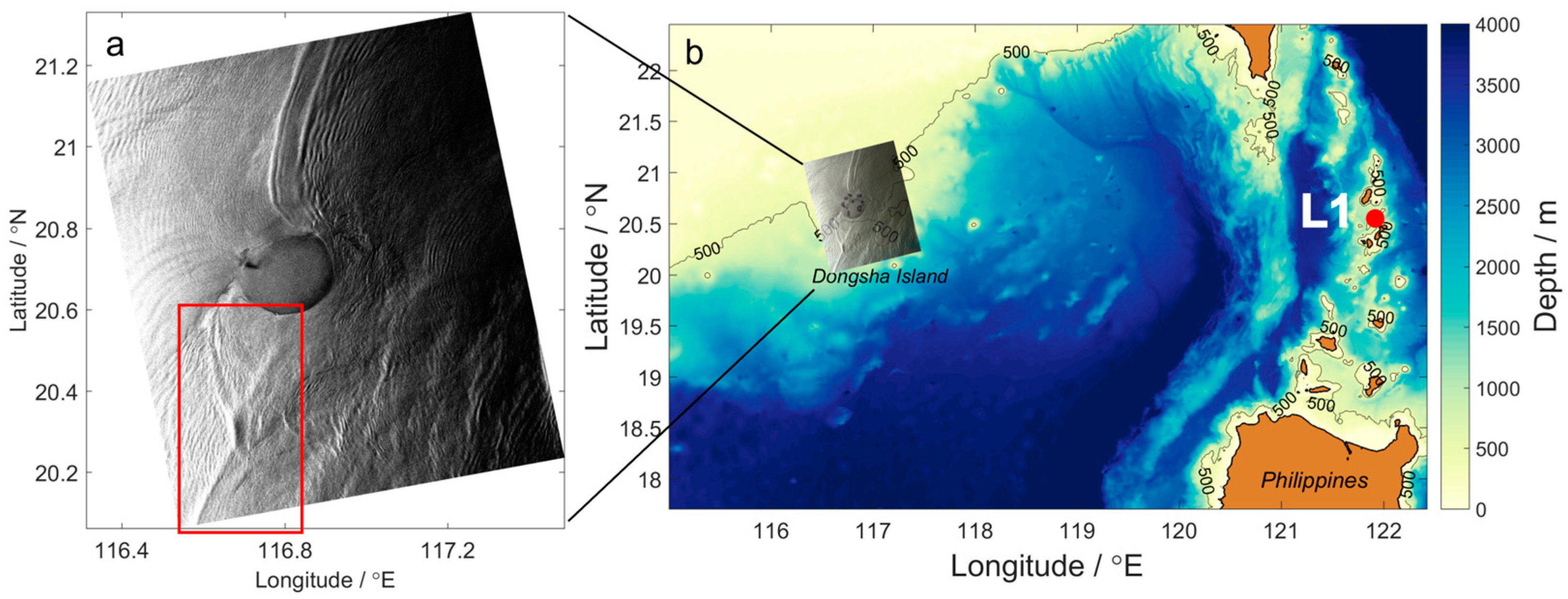
Figure 2.
(a) Vertically averaged zonal velocity over 380 to 450 m depth of the L1 station (eastward is positive): the blue solid line is the simulated model result, and the black dashed line is the observed data [36] (Ramp et al., 2010). (b) SAR image acquired by the ENVISAT satellite at 14:04 on 16 August 2008 UTC; the two red circles indicate the two observed IWs. (c) Map of sea surface height gradient (SSHG) at 39 h of model time; W1 and W2 indicate two IWs.
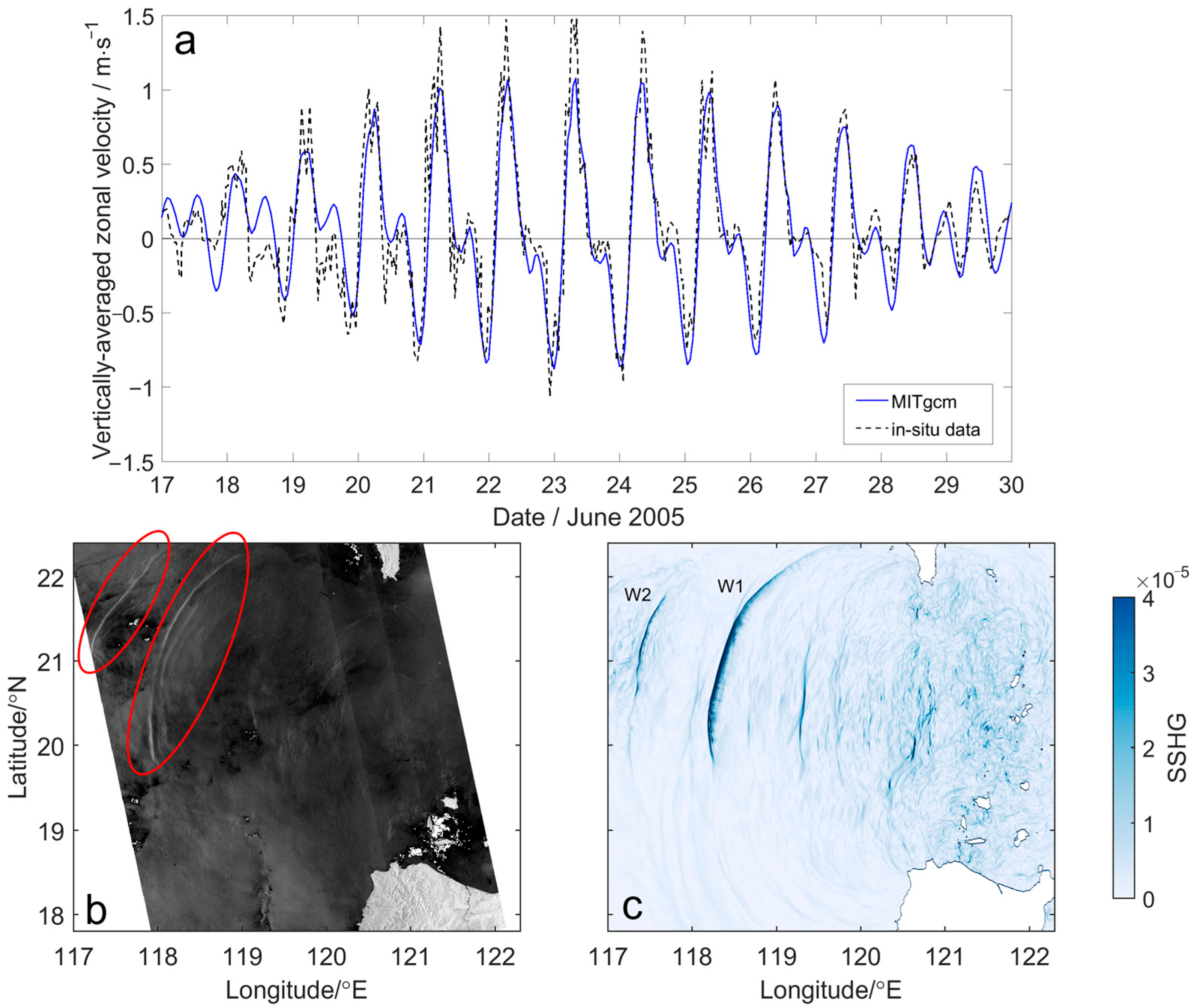
Figure 3.
(a) Map of the sea surface height gradient (SSHG) near Dongsha Island at 52 h 10 min of model time; H1, H2, T1, T2, and IZ, respectively, indicate the cross-sections of two head waves, two tail waves, and the interaction zone. (b) The first three vertical modes of the IWs at cross-section IZ at 52 h 10 min; the red, green, and blue lines, respectively, represent the first, second, and third modes; the black dot indicates the depth of the maximum value of the first mode.
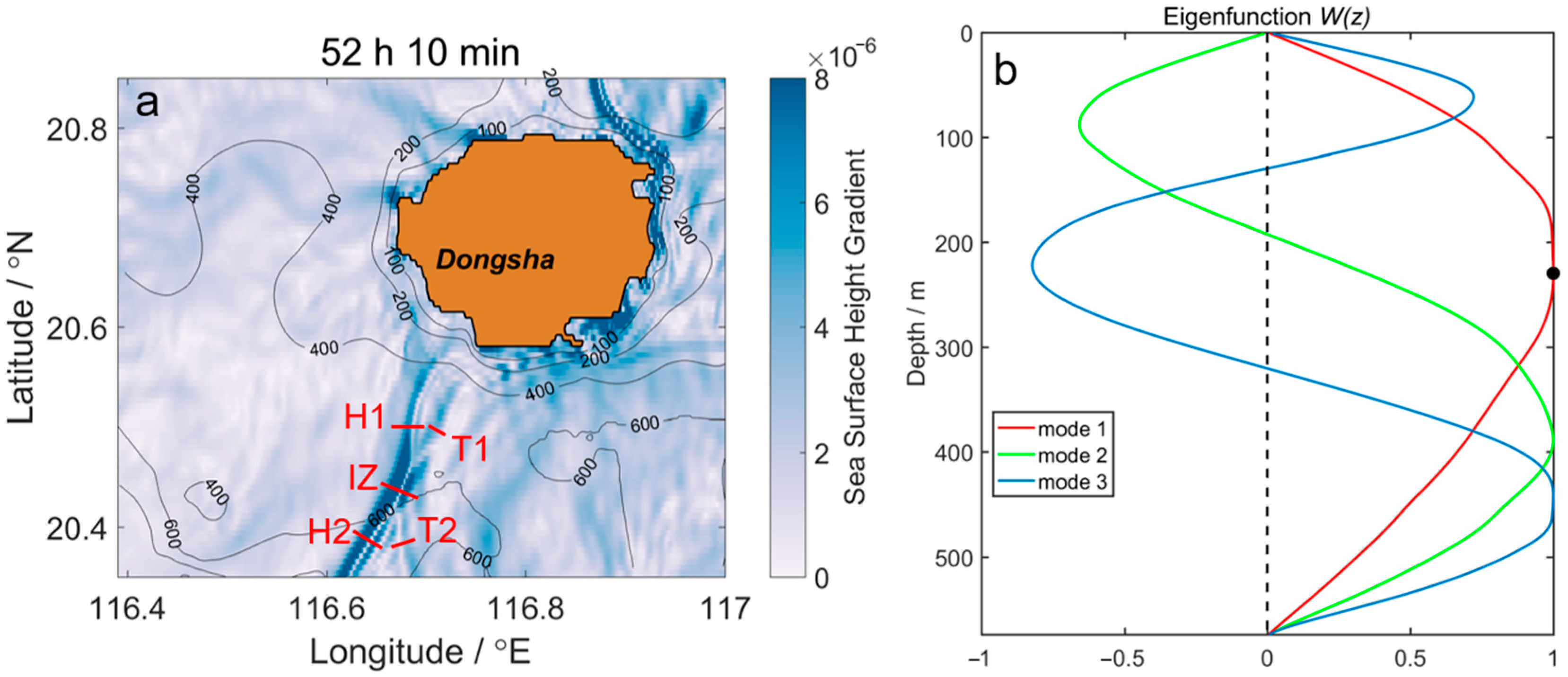
Figure 4.
(a) Overlapped maps of the energy flux at different model times; CS1, CS2, and CS3 are, respectively, the propagation paths of the south head wave, the interaction zone, and the north head wave; purple lines indicate the initial position of the interacted waves. (b) Diagram of the variation of the shape of the waves; orange, blue, and red lines, respectively, represent the north head wave, the south head wave, and the interaction zone, and the thicker the line, the larger the energy flux; the variations are mainly divided into three stages, of which stages 1 and 2 are indicated in brackets with the corresponding time periods in (a).
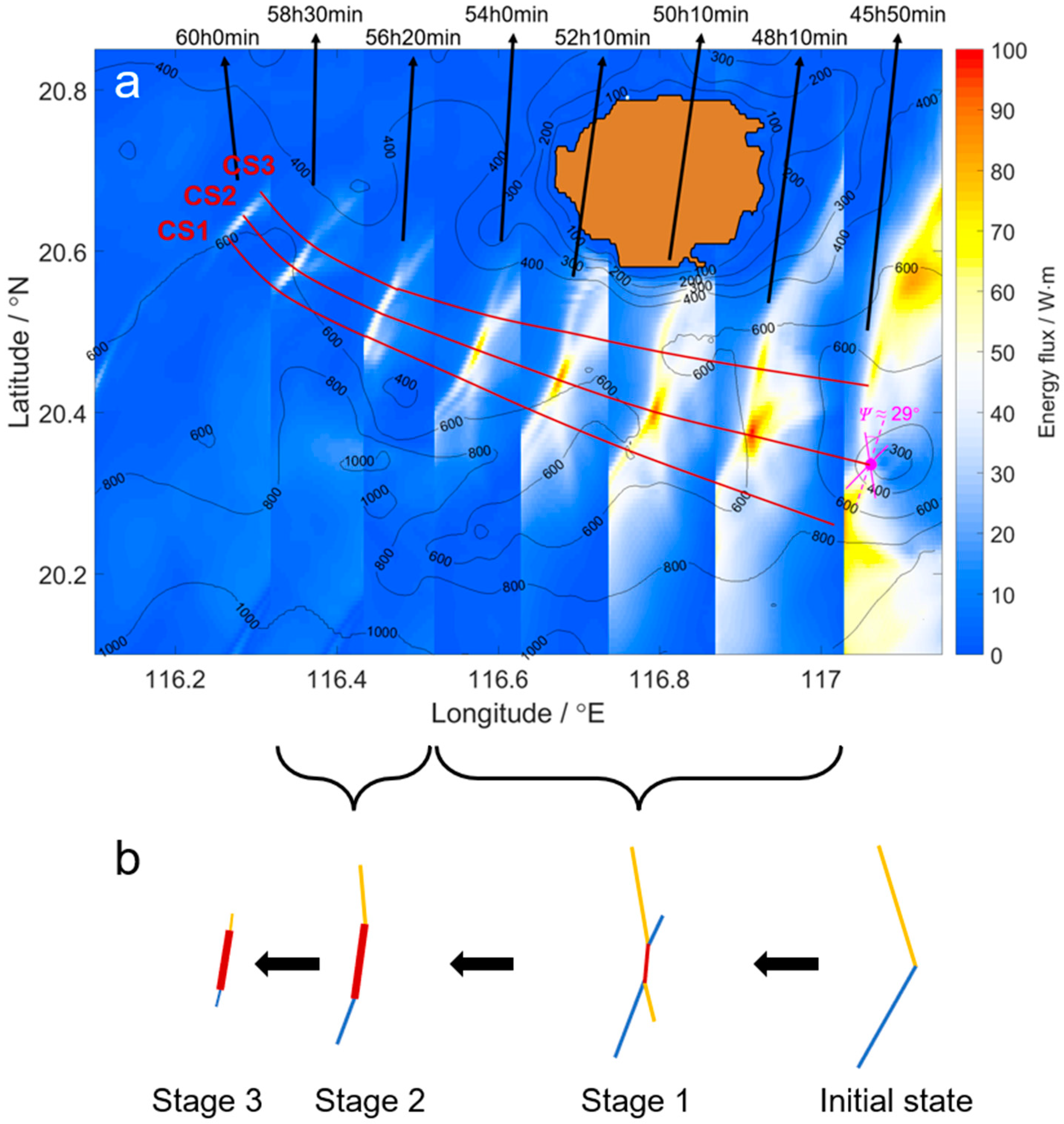
Figure 5.
Map of the energy flux at 52 h 10 min; the two arrows indicate the propagation direction of the gray areas.
Figure 5.
Map of the energy flux at 52 h 10 min; the two arrows indicate the propagation direction of the gray areas.
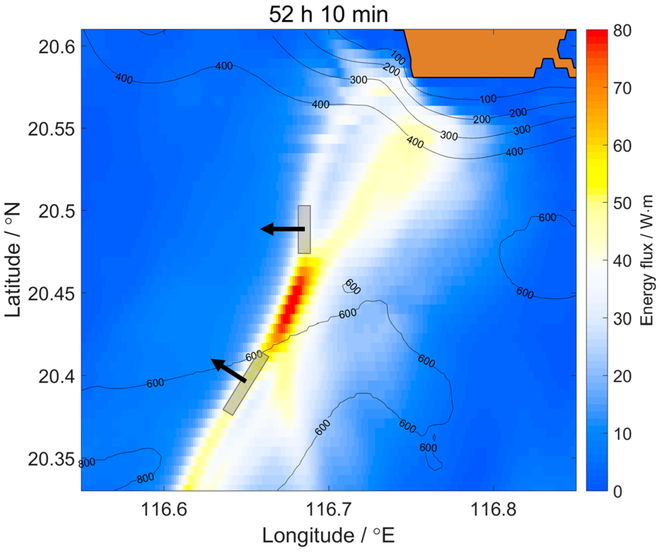
Figure 6.
The temporal variation of the isopycnal displacements (positive value means depression wave) on the sections: (a) CS1, (b) CS2, and (c) CS3 in Figure 4a; the three red rectangles highlight the variation of the interacted waves; the red and black arrows, respectively, indicate the head waves and the tail waves.
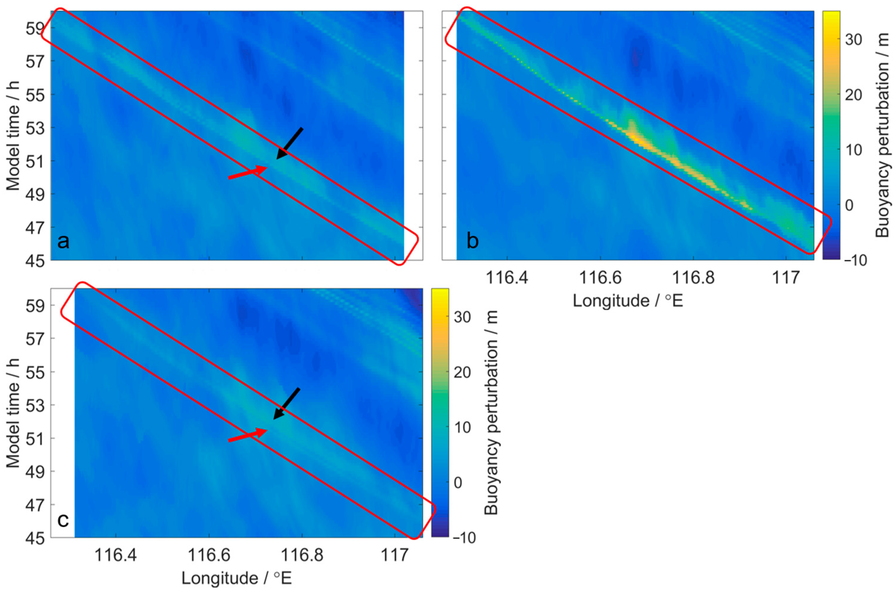
Figure 7.
The variation of (a) the amplitudes of both head waves (model results) and the interaction zone (model result and theoretical value), (b) the angle parameter ψ, (c) the water depth of the section CS2 in Figure 4a, (d) the wave–wave interaction parameter κ; the dashed line means κ = 1; (e) the amplitude amplification parameter as, and (f) the energy flux of the sections CS1, CS2, and CS3 in Figure 4a.
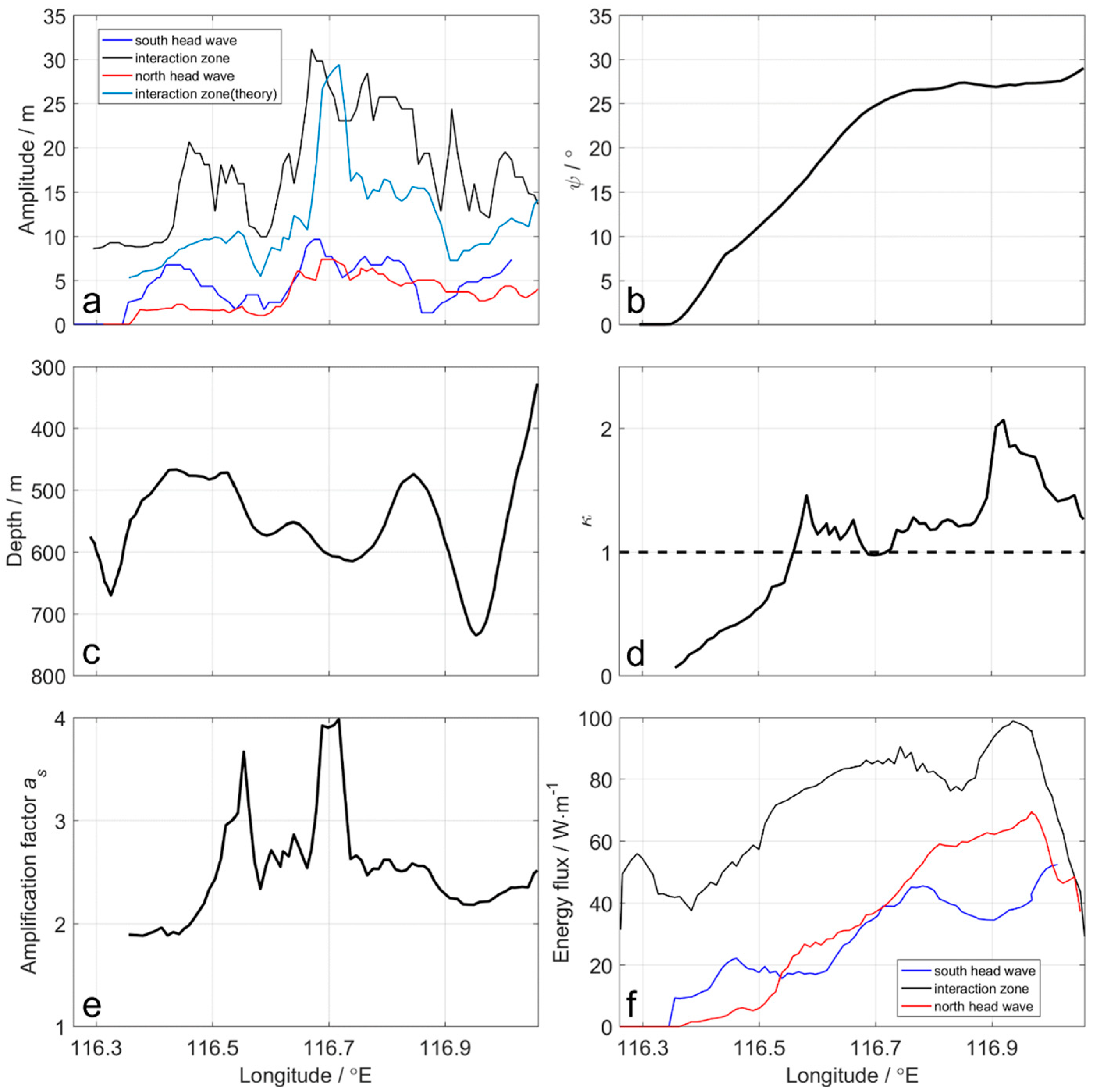
Figure 8.
The temporal variation of the energy flux on the sections: (a) CS1, (b) CS2, and (c) CS3 in Figure 4a; the three red rectangles highlight the variation of the interacted waves.
Figure 8.
The temporal variation of the energy flux on the sections: (a) CS1, (b) CS2, and (c) CS3 in Figure 4a; the three red rectangles highlight the variation of the interacted waves.


Table 1.
Parameters of sections H1, H2, T1, T2, and IZ in Figure 3a.
Table 1.
Parameters of sections H1, H2, T1, T2, and IZ in Figure 3a.
| Section | Water Depth/m | Depth of the Maximum Value of the First Mode/m | Isopycnal Displacement/m |
|---|---|---|---|
| H1 | 492.1 | 208 | 6 |
| H2 | 661.2 | 249 | 9 |
| T1 | 489.4 | 208 | 4 |
| T2 | 633.5 | 244 | 4 |
| IZ | 574.2 | 229 | 30 |
Disclaimer/Publisher’s Note: The statements, opinions and data contained in all publications are solely those of the individual author(s) and contributor(s) and not of MDPI and/or the editor(s). MDPI and/or the editor(s) disclaim responsibility for any injury to people or property resulting from any ideas, methods, instructions or products referred to in the content. |
© 2024 by the authors. Licensee MDPI, Basel, Switzerland. This article is an open access article distributed under the terms and conditions of the Creative Commons Attribution (CC BY) license (https://creativecommons.org/licenses/by/4.0/).
Share and Cite
MDPI and ACS Style
Zeng, Z.; Chen, X.; Yuan, C.; Song, J. A Case Study of Wave–Wave Interaction South to Dongsha Island in the South China Sea. Remote Sens. 2024, 16, 337. https://doi.org/10.3390/rs16020337
AMA Style
Zeng Z, Chen X, Yuan C, Song J. A Case Study of Wave–Wave Interaction South to Dongsha Island in the South China Sea. Remote Sensing. 2024; 16(2):337. https://doi.org/10.3390/rs16020337
Chicago/Turabian StyleZeng, Zhi, Xueen Chen, Chunxin Yuan, and Jun Song. 2024. "A Case Study of Wave–Wave Interaction South to Dongsha Island in the South China Sea" Remote Sensing 16, no. 2: 337. https://doi.org/10.3390/rs16020337
Note that from the first issue of 2016, this journal uses article numbers instead of page numbers. See further details here.