Extracting Shrubland in Deserts from Medium-Resolution Remote-Sensing Data at Large Scale

Abstract

Shrubs are important ecological barriers in desert regions and an important component of global carbon estimation. However, the shrubland in deserts has been hardly presented, although many high-quality land cover datasets with a 10 m scale based on remote-sensing data have been publicly released products. Therefore, the underestimation of carbon storage is inevitable with the absence of desert shrublands. The existing land-cover datasets have been analyzed and compared, and it has been found that the reason for missing the shrubland in deserts is mainly indued by the absence of shrubland samples, which are easy to neglect and difficult to retrieve. In this study, we developed a semi-automatic method to extract shrubland samples in deserts as the updated input for the machine-learning method. Firstly, the initial samples of desert shrublands were identified from the very high spatial-resolution (0.3~0.5 m) imagery on GEE, and the maximum NDVI from Sentinel-2 was used for double-checking. Secondly, a feature-based method was used to learn the feature from the initial samples and a similarity-based searching method was employed to automatically expand the samples. Finally, the expanded samples and their corresponding time-series satellite images were inputted into different machine-learning methods at a large region (1.63 × 10⁶ km²) for extracting the shrubland in the desert. It was found that different combinations of feature variables and time-series combinations have different impacts on the overall accuracy (OA) of the classification results, as well as the performance of identifying and classifying the different land-cover types. Compared to the existing global-scale land-cover products, the proposed method can better identify the shrubland in deserts and show better overall accuracy.

1. Introduction

Perennial shrubs form simple plant communities occupying a large area in desert regions, and they show a unique ability to adapt to the harsh environment of desert ecosystems, which plays an important role in ecosystem stability [1,2]. The monitoring and evaluation of desertification has been a world hotspot and an important way to effectively prevent and control desertification [3]. Desertification research has become a hot issue in multidisciplinary research, and the ability to obtain desert vegetation information quickly and accurately is the basis and key to desertification research. Therefore, mapping the shrub cover in desert areas is of great significance for desertification research.

With the ready availability of remote-sensing data and the advantage of a large area coverage, they have been used for shrub mapping. Since the spatial coverage of shrubs in deserts is usually small [4,5], most of the studies for mapping shrub cover are based on UAV platforms [6,7,8,9] for small areas [5,10,11], which show good results. However, shrub mapping in deserts is usually for much large areas, which is both difficult and very expensive to access UAV data. Therefore, it is economical and practical to produce large-area shrub maps in desert areas through using medium-resolution remote-sensing data.

Laliberte monitored changes of vegetation over time by image segmentation and object-based classification and mapped shrub encroachment in southern New Mexico from 1937 to 2003 [12]. Beck mapped shrub coverage on the North Slope of Alaska at 30 m resolution using a random forest algorithm and compared it with two existing vegetation classification products in the Alaskan Arctic [13]. Baumann demonstrated that a model using both hyperspectral data and SAR images performed much better in mapping shrub coverage than a model using a single image [14]. Bayle used the red-edge band to calculate the normalized anthocyanin reflection index (NARI) and compared its validity with the normalized vegetation index (NDVI) as a basis for shrub vegetation mapping and found that the NARI-based model performed better than the NDVI-based model [15]. Vanselow found that the combination of statistical models and remote-sensing data is more effective in mapping vegetation in arid mountain environments by using the spectral vegetation index MSAVI2 and random forest algorithm [16]. Although these methods have been applied successfully at a specific area, they have not been used at national, continental, and global scales.

Fortunately, some global land-cover products with a medium resolution (10 m or 30 m) are available, such as (1) FROM-GLC10 [17], (2) GLC-FCS30 [18], (3) GlobeLand30 [19], and (4) ESA World Cover [20], which include shrubland. Figure 1 shows the four land-cover maps in Northwestern China covering a large area of desert. It can be seen that the distribution and area of shrubland from each dataset are largely different, which limited the further use of these datasets for research on desertification. Furthermore, all the datasets seem to largely underestimate the areas of the shrubland in deserts. In order to quantitatively evaluate the difference among the above land-cover datasets, we manually interpreted the sampling points based on high-resolution remotely sensed imagery, annual median, and maximum NDVI. The confusion matrix of the land-cover products is listed in

Table A1. Confusion matrix of the land-cover products.

Name	Land Cover Types	OT	BL	GL	SL	PA
GLC-FCS	OT	293	1	30	0	0.904
	BL	205	779	100	20	0.706
	GL	20	0	376	0	0.95
	SL	43	172	17	11	0.005
	UA	0.522	0.818	0.719	0.355
	OA	0.706
FROM-GLC	OT	243	34	47	0	0.75
	BL	6	1084	14	0	0.982
	GL	16	17	361	2	0.912
	SL	1	238	3	1	0.004
	UA	0.914	0.789	0.849	0.333
	OA	0.817
GlobeLand30	OT	286	8	29	1	0.883
	BL	11	944	146	3	0.855
	GL	34	8	349	5	0.881
	SL	1	206	36	0	0
	UA	0.861	0.81	0.623	0
	OA	0.764
ESA World Cover	OT	274	22	24	4	0.846
	BL	5	1062	37	0	0.962
	GL	20	2	374	0	0.944
	SL	0	235	6	2	0.008
	UA	0.916	0.804	0.848	0.333
	OA	0.828

OT = others; BL = bare land; GL = grassland; SL = shrublands; PA = producer accuracy; UA = user accuracy; OA = overall accuracy.

. The overall classification accuracies of GLC-FCS, FROM-GLC, GlobeLand30, and ESA World Cover were 0.706, 0.817, 0.764, and 0.828, respectively. The four land-cover products had a high accuracy in classifying grassland, bareland, and others, but they had variables and low accuracy in classifying shrubland. The above land-cover products are not well-adapted and accurate in the field of desert shrub mapping due to different data sources, classification schemes, and classification methods. Therefore, it remains a challenge to map shrubs in the desert with medium-resolution (10–100 m) remote-sensing data, and it is necessary to study desert shrub mapping by exploring various remote-sensing data and classification algorithms.

The major reasons for identifying the shrubland in the desert at a large scale, such as the global land-cover products, may be concluded as follows:

(1)

Desert shrubs are relatively sparse and have low aggregation, so they are very difficult to be identified through medium-resolution remote-sensing imagery and even high-resolution remote-sensing imagery;

(2)

The areas of shrublands within deserts are very small, so very few samples have been collected while mapping the global land cover by using machine-learning methods, and the samples are too few to learn the characteristics of the shrubland in deserts;

(3)

Although shrub is vegetation, and tools such as the higher vegetation index will show the features of vegetation, the dry conditions in the desert usually depress these features; the input data for global land-cover mapping usually cannot cover the key date of vegetation variation.

In order to better map shrubland in deserts with medium-resolution remote-sensing data, accurately and efficiently collecting the shrubland samples in desert areas is key. In this study, the following steps are made:

Firstly, looking for accurate shrubland samples by using both the very high spatial-resolution data and the time-series data manually.

Secondly, based on the manually retrieved shrubland samples, a method is designed to automatically expand shrubland samples at large scale.

Finally, different machine-learning methods are tested to find the better one for mapping.

2. Study Area and Materials

2.1. Study Area

The study area is in Northern China, which includes Gansu and Qinghai provinces and parts of Inner Mongolia and Xinjiang (Figure 2). The total area is 1.63 × 10⁶ km² with an elevation of −156.8–6834.6 m. There are large areas of low vegetation cover, such as desert, Gobi, and bare soil, as well as areas of high vegetation cover such as grassland and farmland. The climate is mid-temperate continental, with severe cold winters and hot summers, as well as large annual and daily temperature differences.

2.2. Remote-Sensing Data and the Land-Cover Datasets

We selected remote-sensing data at 10 m and 30 m spatial resolution for mapping shrub coverage in desert areas. We collected surface reflectance data from Sentinel-2 for the period from March to October 2020 with less than 30% cloud cover. Sentinel-2 is an Earth observation mission from the Copernicus programme of the European Space Agency and contains two identical satellites: Sentinel-2A and Sentinel-2B. Its spatial resolution of the visible and near-infrared bands is 10 m [21]. The 20 m resolution bands were resampled to 10 m. Data collection and preprocessing is conducted through online code writing on the Google Earth Engine (GEE) cloud platform.

In this study, images with two different kinds of resolution were employed. The very high spatial-resolution images from GEE were used to look for the shrubland in deserts through the texture, and the verified ones corresponded to the Sentinel-2/MSI image through location and the vegetation index variation.

The Copernicus DEM is a Digital Surface Model (DSM), which represents the surface of the Earth including buildings, infrastructure, and vegetation. Digital elevation data were collected and processed on the GEE platform.

ESA World Cover is a global land-cover product at 10 m resolution for 2020, based on both Sentinel-1 and Sentinel-2 data. FROM-GLC is a 10 m resolution global land-cover product derived from the classification of 2017 Sentinel-2 imagery using the Random Forest method. GLC-FCS is a global 30 m resolution surface-coverage product for 2020 based on the 2019–2020 time-series Landsat surface reflectance data, Sentinel-1 SAR data, DEM terrain elevation data, and global thematic ancillary datasets. GlobeLand30 is the 30 m spatial-resolution global surface-coverage data for the year 2020.

3. Methods

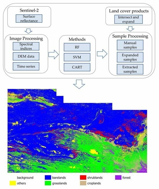
The study is based on remote-sensing classification algorithms and remote-sensing data provided by the GEE cloud platform to map desert shrub coverage. The major procedure of the algorithm is very similar to those algorithms for global land-coverage mapping using Sentinel-2 or Landsat imagery. The major processes include the construction of feature space, machine-learning modules, training data retrieving strategies, and mapping result evaluations. The data processing and analysis flow chart of this study is shown in Figure 3. Besides the similar processes, several modifications have been made in this study specifically for mapping shrublands within deserts, and the modifications include: (1) a small portion of the shrub samples in the deserts are identified manually by using very high spatial-resolution satellite data, and an automatic expansion method is designed for retrieving more shrub samples, which are neglected by most of the global land-cover mapping algorithms; (2) instead of using satellite data with limited temporal information, the time series of images from April to October are employed as the input data; and (3) several machine-learning methods are compared to choose the one with better results.

3.1. Feature Construct

Six remote-sensing spectral indices were calculated to assess the impact of spectral indices on shrub-cover mapping, including normalized difference vegetation index (NDVI) [22], the enhanced vegetation index (EVI) [23], the normalized difference water index (NDWI) [24], the bare soil index (BSI) [25], the normalized difference built-up index (NDBI) [26], and the ratio vegetation index (RVI) [27]. The calculation formulas for each index are as follows:

$$\mathrm{N}\mathrm{D}\mathrm{V}\mathrm{I}=\frac{{\mathrm{R}}_{\mathrm{N}\mathrm{I}\mathrm{R}}-{\mathrm{R}}_{\mathrm{R}\mathrm{E}\mathrm{D}}}{{\mathrm{R}}_{\mathrm{N}\mathrm{I}\mathrm{R}}+{\mathrm{R}}_{\mathrm{R}\mathrm{E}\mathrm{D}}}$$

(1)

$$\mathrm{E}\mathrm{V}\mathrm{I}=2.5\times \frac{{\mathrm{R}}_{\mathrm{N}\mathrm{I}\mathrm{R}}-{\mathrm{R}}_{\mathrm{R}\mathrm{E}\mathrm{D}}}{{\mathrm{R}}_{\mathrm{N}\mathrm{I}\mathrm{R}}+6\times {\mathrm{R}}_{\mathrm{R}\mathrm{E}\mathrm{D}}-7.5\times {\mathrm{R}}_{\mathrm{B}\mathrm{L}\mathrm{U}\mathrm{E}}+1}$$

(2)

$$\mathrm{N}\mathrm{D}\mathrm{W}\mathrm{I}=\frac{{\mathrm{R}}_{\mathrm{G}\mathrm{R}\mathrm{E}\mathrm{E}\mathrm{N}}-{\mathrm{R}}_{\mathrm{S}\mathrm{W}\mathrm{I}\mathrm{R}}}{{\mathrm{R}}_{\mathrm{G}\mathrm{R}\mathrm{E}\mathrm{E}\mathrm{N}}+{\mathrm{R}}_{\mathrm{S}\mathrm{W}\mathrm{I}\mathrm{R}}}$$

(3)

$$\mathrm{B}\mathrm{S}\mathrm{I}=\frac{({\mathrm{R}}_{\mathrm{R}\mathrm{E}\mathrm{D}}+{\mathrm{R}}_{\mathrm{S}\mathrm{W}\mathrm{I}\mathrm{R}})-({\mathrm{R}}_{\mathrm{N}\mathrm{I}\mathrm{R}}+{\mathrm{R}}_{\mathrm{B}\mathrm{L}\mathrm{U}\mathrm{E}})}{\left({\mathrm{R}}_{\mathrm{R}\mathrm{E}\mathrm{D}}+{\mathrm{R}}_{\mathrm{S}\mathrm{W}\mathrm{I}\mathrm{R}}\right)+({\mathrm{R}}_{\mathrm{N}\mathrm{I}\mathrm{R}}+{\mathrm{R}}_{\mathrm{B}\mathrm{L}\mathrm{U}\mathrm{E}})}$$

(4)

$$\mathrm{N}\mathrm{D}\mathrm{B}\mathrm{I}=\frac{{\mathrm{R}}_{\mathrm{S}\mathrm{W}\mathrm{I}\mathrm{R}}-{\mathrm{R}}_{\mathrm{N}\mathrm{I}\mathrm{R}}}{{\mathrm{R}}_{\mathrm{S}\mathrm{W}\mathrm{I}\mathrm{R}}+{\mathrm{R}}_{\mathrm{N}\mathrm{I}\mathrm{R}}}$$

(5)

$$\mathrm{R}\mathrm{V}\mathrm{I}=\frac{{\mathrm{R}}_{\mathrm{N}\mathrm{I}\mathrm{R}}}{{\mathrm{R}}_{\mathrm{R}\mathrm{E}\mathrm{D}}}$$

(6)

where $R_{NIR}$, $R_{RED}$, $R_{\mathrm{B}\mathrm{L}\mathrm{U}\mathrm{E}}$, $R_{GREEN,}$ and $R_{SWIR}$ are the surface-reflectance values of the near-infrared, red, blue, green, and shortwave infrared bands.

3.2. Machine-Learning Modules

Random Forest (RF) algorithm proposed by Leo Beriman [28] is an Ensemble Learning algorithm. The combined multiple weak classifiers generate an average of the final results, so the results of the whole model have high accuracy and generalization performance. It is shown that RF has the advantages of stability, speed, and high accuracy in processing remote-sensing data, so it has important applications in crop extraction, image classification, and agricultural regression modeling [29]. Random forest inherits the idea of bootstrap aggregating, which is an integrated technique for training classifiers on the original dataset by sampling with replacement. It uses a set of trained classifiers to classify the new samples and then uses majority voting or averaging the outputs to count the classification results of all the classifiers, with the category that results in the highest score being the final label.

Support Vector Machines (SVM) [30] is a nonparametric machine-learning algorithm, the core of which is to find an optimal hyperplane as a decision function in a high-dimensional space and, thus, to classify the input vectors into different categories. The choice of kernel function and cost parameter are the most important parameters affecting the performance and efficiency of SVM.

Classification and Regression Tree (CART) [31] is a decision tree that grows in a binary recursive partitioning process, which divides the training dataset into different classes by the maximum variance of the variables within the subset and the minimum variance of the variables within the subset. Where the maximum depth parameter of the tree determines the complexity of the CART model, large depths may have higher accuracy but also increase the risk of overfitting.

3.3. Accuracy Assessment

Overall Accuracy (OA), User Accuracy (UA), and Producer’s Accuracy (PA) are evaluation metrics commonly used for assessing the performance of machine-learning algorithms [32]. The OA and Kappa coefficients adequately reflect the comprehensive accuracy of the results, and the PA and UA can be used to assess the classification accuracy of specific land-cover types.

Classification results were evaluated on a class-by-class basis using a confusion matrix. The final land-cover map produced for the study area was compared with existing land-cover products in the region. The evaluation metrics are calculated, classifiers are implemented, and confusion matrices are computed based on Google Earth Engine [33].

3.4. Training Data-Retrieving Strategy

The quality of the samples used for training or labeling is critical to the accuracy of classification results. The major source of error in many classification processes is inappropriate training samples [34]. Since several global land-cover products have been publicly released, an automated sample extraction strategy from existing land-cover products is proposed, which is economical and efficient. It is assumed that the intersection of the existing products are the samples with high accuracy and high quality.

However, the existing land-cover maps are from different sources, so the number of land-cover types varies, and definitions of the same type of land cover may differ. Subsequently, the land-cover products were resampled to 10 m resolution and converted to a customized classification system (

Table 1. Land-cover classification system.

Code	Class	Abbreviation	Description
1	Others	OT	Other surface types, in addition to the following categories.
2	Bare land	BL	Areas without vegetation cover, including wasteland, deserts, and the Gobi Desert.
3	Grassland	GL	Areas where herbaceous plant cover is greater than 15%, including natural grassland and pastures.
4	Shrubland	SL	Areas in which the shrublands’ height range is 0.3–5 m and cover percentage is >15% have unique texture.
5	Cropland	CL	It varies greatly throughout the year from bare fields to seeding to crop growing to harvesting. It includes paddy fields, greenhouse agriculture, and other types.
6	Forest	FO	Areas with tree cover greater than 15% and tree height greater than 3 m. Includes natural forests, planted forests, and fruit trees.

). In addition, we re-project the four land-cover maps into the same coordinates and crop them into a grid of size 10,000 × 10,000. The intersection of the four land-cover maps for each grid is used. The study area covered a total of 210 grids. Sample points are randomly selected from these grids.

More than enough samples can be retrieved for bare land, grassland, cropland, and forest, but the shrubland is seldom. Consequently, the final result from these training samples hardly maps the shrubland in deserts.

As we know, it is hard to retrieve the shrub samples from the medium-resolution satellite images even with manually checking. By fully taking advantage of high-resolution imagery on GEE platform, we manually collected a small portion of the shrub sample points for training and validation. The high spatial-resolution samples used in this study are Google Earth images. A total of 2067 sample points were randomly sampled in the study area (Figure 4).

Considering the shrubs mainly mixed with bare lands and grasslands in the study area, bare land, grassland, and shrubland were collected as samples. These manually collected samples were incorporated with the samples from the existing land-cover products. Samples were selected from areas where the ground cover has not changed for many years, as well as areas that are relatively homogeneous and little disturbed by human activities, in order to ensure the accuracy and authenticity of the sample data. Figure 5 shows some of the samples’ high-resolution snapshots. However, even at 0.3 m resolution, some of the shrubs cannot be confirmed manually, so the vegetation index at 10 m resolution was also plotted out. Although the extremely dry weather conditions depressed the characteristics of vegetation, the spotted higher vegetation index at the first line of Figure 5 still shows the appearance of the shrubs, which can be used for double confirmation. The spotted vegetation index has obvious difference with the smooth distribution of the vegetation index from bare lands, croplands, and grasslands.

The automated sample extraction strategy from existing land-cover products is shown in Figure 6a. However, the labor-intensive option of collecting highly reliable training samples from interpreting the up-to-date high-resolution images is difficult to implement on a large scale like the study area. Therefore, we use the minimum distance method based on sample similarity to automatically label the samples by using the manually retrieved shrub samples as the initial sample set for feature clustering to achieve spatial expansion of the samples in the study area. The main idea is, for each category, using the existing manual samples, we automatically supervise the labeling of the samples by associating the target categories through the principle of inter-sample similarity to obtain the samples that cover the entire study area. The finalized samples are then applied in the categorization of the study area (Figure 6b).

Mahalanobis distance is a measure of the distance between two data points, considering the covariance structure of the data. It is a multivariate distance metric that considers the correlation between variables.

$$\mathrm{d}(\mathbf{x},\mathbf{y})=\sqrt{{(\mathbf{x}-\mathbf{y})}^{\mathrm{T}}·{\Sigma }^{-1}·(\mathbf{x}-\mathbf{y})}$$

(7)

where x is the vector of the observation and y is the vector of mean values of independent variables, d represents the Mahalanobis distance, and ${\mathsf{\Sigma }}^{-1}$ is the inverse covariance matrix of independent variables.

The final set of training samples consists of a combination of automatically extracted sample points from the existing land-cover products, and the extended samples generated by the above expansion algorithm based on manually verified samples. During training, 20% of samples were randomly selected for validation (

Table 2. Number of total samples and validation samples.

Code	Class	Number of Total Samples	Number of Validation Samples
1	Others	7500	1500
2	Bare land	10,076	2015
3	Grassland	10,550	2110
4	Shrubland	10,550	2110
5	Cropland	8000	1600
6	Forest	7500	1500

). From the extended samples, 2576, 2550, and 2550 bare land, grassland, and shrubland samples were randomly selected and merged with the automatically extracted samples, respectively.

3.5. Time Series Composite

In previous studies, two compositional methods are widely used for land-cover classification using multi-temporal remote-sensing satellite images. One is the use of temporal aggregation, which involves the use of metrics derived from time-series images, such as mean, median, and minimum or maximum values [35,36,37]. Another approach is to combine time series data from all available remote-sensing images [38,39].

Since it is in very dry condition for the study area, the unpredictable precipitation is the key to find vegetation there. Instead of using only a few images, time series of images is employed to capture the vegetation characteristics. However, the noise induced by clouds, cloud shadow, and some other factors will degrade the information, so the maximum, mean, and median of the time-series images or parameters are all calculated, and they are all used as inputs for the RF model.

We created five datasets on the GEE platform with the following temporal aggregation-stacking method. Dataset 1 to Dataset 3 are median, mean, and maximum values of the surface reflectance and spectral index of image, respectively. Dataset 4 and Dataset 5 are median images composed from images of different time ranges. Input images were computed and stacked based on different strategies to assess the impact of different choices on classification accuracy (

Table 3. The composition of datasets used for classification and comparison.

Dataset	Number of Feature Bands	Description
1	16	Median image was composited from April to October of 2020.
2	16	Mean image was composited from April to October of 2020.
3	16	Maximum image was composited from April to October of 2020.
4	45	Median image was composited from April to October and April to July and August to October of 2020.
5	52	Image composited from Dataset 4 and spectral indices of Dataset 3.

).

4. Results

4.1. Influence of the Feature Variables on the Classification Accuracy

In this part, we tested the classification accuracy of the three classification algorithms based on Dataset 1 in Table 3 with different combinations of features.

Table 4. Influences of different combinations of feature variables on producer accuracy (PA).

Land Cover Types	Spectral Bands			Spectral Bands + Spectral Indices			Spectral Bands + Spectral Indices + DEM
	RF	SVM	CART	RF	SVM	CART	RF	SVM	CART
OT	0.876	0.779	0.824	0.867	0.761	0.828	0.893	0.782	0.844
BL	0.933	0.856	0.829	0.935	0.879	0.836	0.96	0.876	0.872
GL	0.654	0.391	0.560	0.656	0.420	0.578	0.778	0.485	0.658
SL	0.693	0.670	0.461	0.706	0.677	0.499	0.801	0.672	0.569
CL	0.670	0.490	0.480	0.708	0.513	0.510	0.770	0.526	0.593
FO	0.815	0.834	0.754	0.821	0.801	0.776	0.857	0.853	0.806

OT = others; BL = bare land; GL = grassland; SL = shrubland; CL = cropland; FO = forest.

and

Table 5. Influences of different combinations of feature variables on user accuracy (UA).

Land Cover Types	Spectral Bands			Spectral Bands + Spectral Indices			Spectral Bands + Spectral Indices + DEM
	RF	SVM	CART	RF	SVM	CART	RF	SVM	CART
OT	0.914	0.813	0.830	0.924	0.824	0.824	0.942	0.826	0.854
BL	0.900	0.786	0.831	0.897	0.763	0.846	0.921	0.769	0.868
GL	0.625	0.506	0.557	0.640	0.535	0.581	0.755	0.587	0.653
SL	0.701	0.534	0.445	0.714	0.557	0.461	0.792	0.552	0.545
CL	0.682	0.577	0.482	0.702	0.543	0.522	0.784	0.579	0.602
FO	0.833	0.758	0.767	0.834	0.789	0.792	0.880	0.821	0.820

OT = others; BL = bare land; GL = grassland; SL = shrubland; CL = cropland; FO = forest.

show the producer accuracy and user accuracy from the classification results for different combination of feature variables and machine-learning algorithms.

Forest, others, and bare land generally had higher accuracy and were less affected by combinations of input feature variables, while land-cover types such as cropland, shrubland, and grasslands were more affected by combinations of characterization variables. When the RF classifier was used, the spectral indices had a weak effect on improving the classification accuracy for bare land, grassland, and shrubland, with accuracy increases by 0.01–0.03, the DEM data had a significant impact on the improvement of classification accuracy for bare land, grassland, and shrubland, with accuracy increases by 0.08–0.12. When the SVM classifier was used, the spectral indices and the DEM data had a weak effect on improving the classification accuracy for bare land, grassland, and shrubland, while accuracy may increase or decrease. When the CART classifier was used, the spectral indices and the DEM data had a weak effect on improving the classification accuracy for bare land, grassland, and shrubland, with accuracy increases by 0.03–0.07.

4.2. Influence of the Times-Series Data on the Classification Accuracy

Based on the results in the previous subsection, we chose to use the Random Forest algorithm to verify the effect of datasets composed of different time series on the accuracy of land-cover classification.

Figure A1 shows the distribution of importance scores for all input feature variables involved in classification in different datasets. Different characteristic variables in random forests have different importance in participating in classification, and variables with higher importance scores contribute more to the classification results [40]. From the figure, it can be seen that DEM feature, RVI, and NDVI feature have higher importance scores, while spectral bands and other spectral indices have lower importance scores. Spectral bands B4 and B11 generally have higher importance scores than other spectral bands. The importance scores of the spectral indices NDVI and RVI were generally higher than the other spectral indices.

Dataset 1, Dataset 2, and Dataset 3 were composited from all the images with less than 30% cloud cover in the study area from April to October in 2020, and the compositing methods were median, mean, and maximum values, respectively. Dataset 4 is a combination of Dataset 1 and the median of images with less than 30% cloud cover in the study area from April to July 2020 and August to October 2020. Dataset 5 is a combination of Dataset 4 and spectral indices of Dataset 3. Dataset 4 and Dataset 5 had the highest OA of 0.88 and 0.891, respectively, followed by Dataset 2 (0.854), Dataset 1 (0.835), and Dataset 3 (0.811). Meanwhile, bare land, grassland, and shrubland have the highest PA and UA in Dataset 5 (

Table 6. UA, PA, and OA of land-cover types from the classification results of the five different datasets.

		OT	BL	GL	SL	CL	FO	Kappa	OA
Dataset 1	PA	0.893	0.960	0.778	0.801	0.770	0.857	0.801	0.835
	UA	0.942	0.921	0.755	0.792	0.784	0.880
Dataset 2	PA	0.911	0.960	0.790	0.801	0.819	0.889	0.824	0.854
	UA	0.935	0.935	0.769	0.821	0.818	0.895
Dataset 3	PA	0.888	0.934	0.725	0.740	0.779	0.855	0.773	0.811
	UA	0.909	0.915	0.716	0.772	0.765	0.843
Dataset 4	PA	0.903	0.982	0.820	0.842	0.846	0.922	0.855	0.880
	UA	0.957	0.940	0.809	0.872	0.828	0.915
Dataset 5	PA	0.915	0.981	0.830	0.848	0.873	0.932	0.869	0.891
	UA	0.965	0.947	0.816	0.882	0.859	0.918

OT = others; BL = bare land; GL = grassland; SL = shrubland; CL = cropland; FO = forest; PA = producer accuracy; UA = user accuracy; OA = overall accuracy; Kappa = Kappa coefficient.

).

Comparing the results of Dataset 1, Dataset 2, and Dataset 3, Dataset 2 has consistently higher accuracy for PA and UA for all land-cover types, Dataset 1 is slightly lower than Dataset 2, and Dataset 3 has the lowest accuracy. Therefore, the median and mean are better choices than the maximum if images within a year need to be composited. The accuracy of the land-cover types in Dataset 4 improved compared to Datasets 1 to 3, with the greatest improvement being in shrubland and cropland. This indicates that stacking composited data from different time periods helps to improve the accuracy of land-cover types that are difficult to classify. Meanwhile stacking different types of composited data can also improve the accuracy of classification. Therefore, the use of both median and time-series compositions, as well as spectral indices and DEM data, should be considered in applications.

4.3. Classification Results

In order to evaluate the land-cover results obtained in this study, the classification results were compared with existing high spatial-resolution land-cover products, including FROM-GLC, GLC-FCS, ESA Word Cover, and GlobeLand30.

Figure 7 shows the confusion matrix for the classification results using samples from different sources. Manually verified sample sets are used to validate the classification results. When using only the sample extracted from the available land-cover data, the highest PA(RECALL) was 90.74% for other, and after adding the expansion samples, the highest PA was 92.3%, 94.4%, and 78.19% for bare land, grassland, and shrubs, respectively. When combining the two samples, other, bare ground, grass, and shrubs had the highest UA(PERCISION) of 78.86%, 96.4%, 87.79%, and 88.37%, respectively.

Figure 8 shows a visual comparison of the classification images of the random forest trained by the two sample sets. Figure 9 and Figure 10 show a visual comparison of the classification results obtained in this study with the existing land-cover products in several different magnification regions. The different land-cover products showed great differences in areas with complex land-cover types. Therefore, we chose areas with complex land-cover types, including shrublands, grasslands, forests, and croplands as the magnification regions in the study area. It can be seen that the classification effect of the land-cover results obtained in this study has been significantly improved. For example, in terms of recognizing and classifying artificial surfaces, ESA Word Cover is prone to misclassify roads as bare ground (Figure 8F and Figure 9D). In addition, the classification results of this study resulted in a more accurate identification of land-cover-type boundaries and more shrubland cover than these products. Samples obtained from existing land-cover products lacked the sparse shrub cover found in deserts. Expanding a small number of hand-collected samples solved this problem well, and as can be seen in Figure 9A,B,E, many of the sparse shrubs categorized as bare ground were also extracted using the expanded samples.

From the mapping result, bare lands, grasslands, shrublands, croplands, and forests accounted for 59.35%, 21.57%, 4.23%, 3.98%, and 1.72% of the area of the study area, respectively. Shrubs are mainly located in the transition zone between desert bare ground and grassland.

5. Discussion

Comparing the shrubland results for the four land-cover products, we found that FROM-GLC, GlobeLand30, and ESA World Cover had a very low percentage of sparse desert shrublands in the study area, and GLC-FCS contained more shrublands. The four land-cover products showed low consistency in the proportion of shrublands and distribution. Therefore, the accuracy of the global land-cover products on shrubland in desert areas is very low, and medium-resolution satellite imagery is very difficult to capture the characteristics of shrubland in deserts. However, it is not impossible to retrieve more information on shrubland in deserts from medium-resolution satellite imagery.

An analysis of three classification algorithms, Support Vector Machine (SVM), Categorical Regression Tree (CART), and Random Forest (RF), reveals that the RF algorithm has a significant advantage when using a large number of features and samples for classification. A comparison of the classification accuracies revealed that all three remote-sensing classification algorithms were accurate for other, bare land, and forest, but less accurate for grasslands, shrublands, and croplands. This is because land-cover types such as grassland and cropland are highly seasonal, and shrubs often grow in tandem with grassland and bare ground. Surprisingly, SVM’s classification results are of low quality, which is inconsistent with some past studies that found SVM to be the most accurate classifier [41,42]. The different geographical locations and climates of the study areas of these studies, the different topographic features, and the different definitions of land-cover types caused the different results. Different satellites also have different sensors and time periods for acquiring data, which also leads to different results from different classification algorithms.

The use of spectral indices and topographic features improved the classification accuracy of random forests, with NDVI, elevation, and RVI having the strongest feature importance (Table 4 and Table 5, and Figure A1). This is consistent with other findings, such as reports that spectral indices (e.g., NDVI, EVI, and SAVI) improve the accuracy of land-cover classification [43]. The DEM data resulted in a maximum improvement of 0.12 in classification accuracy for bare lands, grasslands, and shrublands. There is a strong correlation between land-cover type and elevation, which indicates that elevation makes it easier to differentiate between grassland and other vegetation or bare ground, as well as between bare ground and man-made built-up areas.

The median composite method can be used on the GEE platform to quickly process hundreds of images and filter out images with less than 30% cloud cover. A single cloud-free image of a certain time period is obtained from the image collection by extracting the median value of the surface reflectance. In addition to the median method, other methods such as mean and maximum are also used. The results of Dataset 4 and Dataset 5 show that overlaying different types of annual composites and multiple monthly composites helps to improve the classification results. Due to the movement of clouds, the composition of the median of the image in different years or in different regions affects the acquisition of phenological information. For example, in 2020, a large portion of the southwestern region of the study area was covered by clouds for a long period of time from April to July, leaving information for the rest of the year when the median was computed. This effect is severe for study areas with strong seasonality in land-cover types.

In the lack of a large number of samples, large-scale land-cover classification mapping was accomplished by extracting samples using existing high-quality land-cover classification datasets. In the case of a few shrub samples in the study area, better classification results can also be achieved by making use of similar samples from different spatial locations for training and expanding samples from manually collected samples.

Since this study succeeded in mapping a large portion of shrubland in deserts compared to the previous global land-cover products, the trained model parameters will be applied for shrubland mapping at other areas at first, and an automated procedure will be developed to evaluate the results for selecting more samples to retrain the model to improve the mapping results.

6. Conclusions

Medium-scale remote-sensing images are easy to acquire and cover a wide range of areas, which is suitable for large-scale land-cover studies. However, the machine-learning-based products cannot identify the sparsely distributed land cover with small size, such as the shrubland in deserts, which is due to the missing samples for these land covers. Fortunately, with the high-resolution images on Google Earth Engine, a small portion of samples for shrubs in deserts can be recognized and can also be double confirmed through the vegetation characteristics from medium-resolution remote-sensing data. Therefore, a semi-automatic method for collecting shrub samples in deserts is proposed to train different machine-learning modules, and the proposed procedure can achieve an overall accuracy of 90.66% and a 15.2% higher rate than that without shrub samples. Especially, the PA and UA for the shrubland are 78.19% and 88.37%, which is close to 0 for other products. In near future, this method will be employed to retrieve the global shrublands in deserts and to improve the accuracy of shrubland for the existing land-cover products.

References

- Sun, Q.; Zhang, P.; Wei, H.; Liu, A.; You, S.; Sun, D. Improved Mapping and Understanding of Desert Vegetation-Habitat Complexes from Intraannual Series of Spectral Endmember Space Using Cross-Wavelet Transform and Logistic Regression. Remote Sens. Environ. 2020, 236, 111516. [Google Scholar] [CrossRef]
- Yao, Y.; Zhao, Z.; Wei, X.; Shao, M. Effects of Shrub Species on Soil Nitrogen Mineralization in the Desert-Loess Transition Zone. Catena 2019, 173, 330–338. [Google Scholar] [CrossRef]
- Rogan, J.; Chen, D. Remote Sensing Technology for Mapping and Monitoring Land-Cover and Land-Use Change. Prog. Plan. 2004, 61, 301–325. [Google Scholar] [CrossRef]
- Brandt, M.; Hiernaux, P.; Tagesson, T.; Verger, A.; Rasmussen, K.; Diouf, A.A.; Mbow, C.; Mougin, E.; Fensholt, R. Woody Plant Cover Estimation in Drylands from Earth Observation Based Seasonal Metrics. Remote Sens. Environ. 2016, 172, 28–38. [Google Scholar] [CrossRef]
- Cao, X.; Liu, Y.; Liu, Q.; Cui, X.; Chen, X.; Chen, J. Estimating the Age and Population Structure of Encroaching Shrubs in Arid/Semiarid Grasslands Using High Spatial Resolution Remote Sensing Imagery. Remote Sens. Environ. 2018, 216, 572–585. [Google Scholar] [CrossRef]
- Zhou, H.; Fu, L.; Sharma, R.P.; Lei, Y.; Guo, J. A Hybrid Approach of Combining Random Forest with Texture Analysis and VDVI for Desert Vegetation Mapping Based on UAV RGB Data. Remote Sens. 2021, 13, 1891. [Google Scholar] [CrossRef]
- Zhang, T.; Bi, Y.; Du, J.; Zhu, X.; Gao, X. Classification of Desert Grassland Species Based on a Local-Global Feature Enhancement Network and UAV Hyperspectral Remote Sensing. Ecol. Inform. 2022, 72, 101852. [Google Scholar] [CrossRef]
- Mao, P.; Qin, L.; Hao, M.; Zhao, W.; Luo, J.; Qiu, X.; Xu, L.; Xiong, Y.; Ran, Y.; Yan, C.; et al. An Improved Approach to Estimate Above-Ground Volume and Biomass of Desert Shrub Communities Based on UAV RGB Images. Ecol. Indic. 2021, 125, 107494. [Google Scholar] [CrossRef]
- Al-Ali, Z.M.; Abdullah, M.M.; Asadalla, N.B.; Gholoum, M. A Comparative Study of Remote Sensing Classification Methods for Monitoring and Assessing Desert Vegetation Using a UAV-Based Multispectral Sensor. Environ. Monit. Assess. 2020, 192, 389. [Google Scholar] [CrossRef]
- Sun, B.; Li, Z.; Gao, W.; Zhang, Y.; Gao, Z.; Song, Z.; Qin, P.; Tian, X. Identification and Assessment of the Factors Driving Vegetation Degradation/Regeneration in Drylands Using Synthetic High Spatiotemporal Remote Sensing Data—A Case Study in Zhenglanqi, Inner Mongolia, China. Ecol. Indic. 2019, 107, 105614. [Google Scholar] [CrossRef]
- Peng, H.Y.; Li, X.; Tong, S. Effects of Shrub Encroachment on Biomass and Biodiversity in the Typical Steppe of Inner Mongolia. Acta Ecol. Sin. 2013, 33, 7221–7229. [Google Scholar] [CrossRef]
- Laliberte, A.S.; Rango, A.; Havstad, K.M.; Paris, J.F.; Beck, R.F.; McNeely, R.; Gonzalez, A.L. Object-Oriented Image Analysis for Mapping Shrub Encroachment from 1937 to 2003 in Southern New Mexico. Remote Sens. Environ. 2004, 93, 198–210. [Google Scholar] [CrossRef]
- Beck, P.S.A.; Horning, N.; Goetz, S.J.; Loranty, M.M.; Tape, K.D. Shrub Cover on the North Slope of Alaska: A circa 2000 Baseline Map. Arct. Antarct. Alp. Res. 2011, 43, 355–363. [Google Scholar] [CrossRef]
- Baumann, M.; Levers, C.; Macchi, L.; Bluhm, H.; Waske, B.; Gasparri, N.I.; Kuemmerle, T. Mapping Continuous Fields of Tree and Shrub Cover across the Gran Chaco Using Landsat 8 and Sentinel-1 Data. Remote Sens. Environ. 2018, 216, 201–211. [Google Scholar] [CrossRef]
- Bayle, A.; Carlson, B.Z.; Thierion, V.; Isenmann, M.; Choler, P. Improved Mapping of Mountain Shrublands Using the Sentinel-2 Red-Edge Band. Remote Sens. 2019, 11, 2807. [Google Scholar] [CrossRef]
- Vanselow, K.A.; Samimi, C. Predictive Mapping of Dwarf Shrub Vegetation in an Arid High Mountain Ecosystem Using Remote Sensing and Random Forests. Remote Sens. 2014, 6, 6709–6726. [Google Scholar] [CrossRef]
- Gong, P.; Liu, H.; Zhang, M.; Li, C.; Wang, J.; Huang, H.; Clinton, N.; Ji, L.; Li, W.; Bai, Y.; et al. Stable Classification with Limited Sample: Transferring a 30-m Resolution Sample Set Collected in 2015 to Mapping 10-m Resolution Global Land Cover in 2017. Sci. Bull. 2019, 64, 3. [Google Scholar] [CrossRef]
- Zhang, X.; Liu, L.; Chen, X.; Gao, Y.; Xie, S.; Mi, J. GLC_FCS30: Global Land-Cover Product with Fine Classification System at 30 m Using Time-Series Landsat Imagery. Earth Syst. Sci. Data 2021, 13, 2753–2776. [Google Scholar] [CrossRef]
- Chen, J.; Chen, J.; Liao, A.; Cao, X.; Chen, L.; Chen, X.; He, C.; Han, G.; Peng, S.; Lu, M.; et al. Global Land Cover Mapping at 30m Resolution: A POK-Based Operational Approach. ISPRS J. Photogramm. Remote Sens. 2015, 103, 7–27. [Google Scholar] [CrossRef]
- Zanaga, D.; Van De Kerchove, R.; De Keersmaecker, W.; Souverijns, N.; Brockmann, C.; Quast, R.; Wevers, J.; Grosu, A.; Paccini, A.; Vergnaud, S.; et al. ESA WorldCover 10 m 2020 V100 2021. Available online: https://zenodo.org/records/5571936 (accessed on 1 June 2023).
- Drusch, M.; Del Bello, U.; Carlier, S.; Colin, O.; Fernandez, V.; Gascon, F.; Hoersch, B.; Isola, C.; Laberinti, P.; Martimort, P.; et al. Sentinel-2: ESA’s Optical High-Resolution Mission for GMES Operational Services. Remote Sens. Environ. 2012, 120, 25–36. [Google Scholar] [CrossRef]
- Huang, S.; Tang, L.; Hupy, J.P.; Wang, Y.; Shao, G. A Commentary Review on the Use of Normalized Difference Vegetation Index (NDVI) in the Era of Popular Remote Sensing. J. For. Res. 2021, 32, 1–6. [Google Scholar] [CrossRef]
- Son, N.T.; Chen, C.F.; Chen, C.R.; Minh, V.Q.; Trung, N.H. A Comparative Analysis of Multitemporal MODIS EVI and NDVI Data for Large-Scale Rice Yield Estimation. Agric. For. Meteorol. 2014, 197, 52–64. [Google Scholar] [CrossRef]
- Gao, B. NDWI—A Normalized Difference Water Index for Remote Sensing of Vegetation Liquid Water from Space. Remote Sens. Environ. 1996, 58, 257–266. [Google Scholar] [CrossRef]
- Rasul, A.; Balzter, H.; Ibrahim, G.R.F.; Hameed, H.M.; Wheeler, J.; Adamu, B.; Ibrahim, S.; Najmaddin, P.M. Applying Built-Up and Bare-Soil Indices from Landsat 8 to Cities in Dry Climates. Land 2018, 7, 81. [Google Scholar] [CrossRef]
- Zhang, Y.; Odeh, I.O.A.; Han, C. Bi-Temporal Characterization of Land Surface Temperature in Relation to Impervious Surface Area, NDVI and NDBI, Using a Sub-Pixel Image Analysis. Int. J. Appl. Earth Obs. Geoinf. 2009, 11, 256–264. [Google Scholar] [CrossRef]
- Gonenc, A.; Ozerdem, M.S.; Acar, E. Comparison of NDVI and RVI Vegetation Indices Using Satellite Images. In Proceedings of the 2019 8th International Conference on Agro-Geoinformatics (Agro-Geoinformatics), Istanbul, Turkey, 16–19 July 2019; IEEE: Piscataway, NJ, USA, 2019; pp. 1–4. [Google Scholar]
- Parmar, A.; Katariya, R.; Patel, V. A Review on Random Forest: An Ensemble Classifier. In International Conference on Intelligent Data Communication Technologies and Internet of Things (ICICI) 2018; Hemanth, J., Fernando, X., Lafata, P., Baig, Z., Eds.; Lecture Notes on Data Engineering and Communications Technologies; Springer International Publishing: Cham, Switzerland, 2019; Volume 26, pp. 758–763. ISBN 978-3-030-03145-9. [Google Scholar]
- Belgiu, M.; Drăguţ, L. Random Forest in Remote Sensing: A Review of Applications and Future Directions. ISPRS J. Photogramm. Remote Sens. 2016, 114, 24–31. [Google Scholar] [CrossRef]
- Shao, Y.; Lunetta, R.S. Comparison of Support Vector Machine, Neural Network, and CART Algorithms for the Land-Cover Classification Using Limited Training Data Points. ISPRS J. Photogramm. Remote Sens. 2012, 70, 78–87. [Google Scholar] [CrossRef]
- Bittencourt, H.R.; Clarke, R.T. Use of Classification and Regression Trees (CART) to Classify Remotely-Sensed Digital Images. In Proceedings of the IGARSS 2003. 2003 IEEE International Geoscience and Remote Sensing Symposium. Proceedings (IEEE Cat. No.03CH37477), Toulouse, France, 21–25 July 2003; Volume 6, pp. 3751–3753. [Google Scholar]
- Congalton, R.G. A Review of Assessing the Accuracy of Classifications of Remotely Sensed Data. Remote Sens. Environ. 1991, 37, 35–46. [Google Scholar] [CrossRef]
- Gorelick, N.; Hancher, M.; Dixon, M.; Ilyushchenko, S.; Thau, D.; Moore, R. Google Earth Engine: Planetary-Scale Geospatial Analysis for Everyone. Remote Sens. Environ. 2017, 202, 18–27. [Google Scholar] [CrossRef]
- Pal, M.; Mather, P.M. Some Issues in the Classification of DAIS Hyperspectral Data. Int. J. Remote Sens. 2006, 27, 2895–2916. [Google Scholar] [CrossRef]
- Beckschäfer, P. Obtaining Rubber Plantation Age Information from Very Dense Landsat TM & ETM+ Time Series Data and Pixel-Based Image Compositing. Remote Sens. Environ. 2017, 196, 89–100. [Google Scholar] [CrossRef]
- Xie, S.; Liu, L.; Zhang, X.; Yang, J.; Chen, X.; Gao, Y. Automatic Land-Cover Mapping Using Landsat Time-Series Data Based on Google Earth Engine. Remote Sens. 2019, 11, 3023. [Google Scholar] [CrossRef]
- Zeng, L.; Wardlow, B.D.; Xiang, D.; Hu, S.; Li, D. A Review of Vegetation Phenological Metrics Extraction Using Time-Series, Multispectral Satellite Data. Remote Sens. Environ. 2020, 237, 111511. [Google Scholar] [CrossRef]
- Griffiths, P.; van der Linden, S.; Kuemmerle, T.; Hostert, P. A Pixel-Based Landsat Compositing Algorithm for Large Area Land Cover Mapping. IEEE J. Sel. Top. Appl. Earth Obs. Remote Sens. 2013, 6, 2088–2101. [Google Scholar] [CrossRef]
- Hermosilla, T.; Wulder, M.A.; White, J.C.; Coops, N.C.; Hobart, G.W. Disturbance-Informed Annual Land cover Classification Maps of Canada’s Forested Ecosystems for a 29-Year Landsat Time Series. Can. J. Remote Sens. 2018, 44, 67–87. [Google Scholar] [CrossRef]
- Archer, K.J.; Kimes, R.V. Empirical Characterization of Random Forest Variable Importance Measures. Comput. Stat. Data Anal. 2008, 52, 2249–2260. [Google Scholar] [CrossRef]
- Rana, V.K.; Venkata Suryanarayana, T.M. Performance Evaluation of MLE, RF and SVM Classification Algorithms for Watershed Scale Land Use/Land Cover Mapping Using Sentinel 2 Bands. Remote Sens. Appl. Soc. Environ. 2020, 19, 100351. [Google Scholar] [CrossRef]
- Mountrakis, G.; Im, J.; Ogole, C. Support Vector Machines in Remote Sensing: A Review. ISPRS J. Photogramm. Remote Sens. 2011, 66, 247–259. [Google Scholar] [CrossRef]
- Zhang, Z.; Wei, M.; Pu, D.; He, G.; Wang, G.; Long, T. Assessment of Annual Composite Images Obtained by Google Earth Engine for Urban Areas Mapping Using Random Forest. Remote Sens. 2021, 13, 748. [Google Scholar] [CrossRef]
Figure 1.
Land-cover maps of the study area used in this paper. (a) GLC-FCS; (b) FROM-GLC; (c) GlobeLand30; (d) ESA World Cover.
Figure 2.
Location of the study area.
Figure 3.
Flowchart of data processing and analysis.
Figure 4.
Distribution of sample points in the study area.
Figure 5.
High-resolution imagery of shrublands, grasslands, croplands, and bare lands.
Figure 6.
Algorithm details for expanding samples. (a) Methods for obtaining samples based on existing land-cover products. (b) Methods for expanding manually created sample sets.
Figure 7.
The confusion matrices computed using manual samples. (a) OURS-ES means results obtained using a random forest trained with a mixture of expanded samples and extracted samples from existing products. (b) OURS-NES means results obtained using a random forest trained with samples only from existing products. The red letters in the graph represent the overall accuracies.
Figure 8.
The classification results of this study are compared with areas of existing high spatial-resolution land-cover products. (a) OURS-ES, (b) OURS-NES.
Figure 9.
The classification results of this study compared with areas of existing land-cover products ((A), 39.8974076°N, 106.3292915°E; (B), 41.2157217°N, 97.7361003°E; (C), 43.5114046°N, 93.4742268°E; (D), 35.1575914°N, 105.8086764°E; (E), 42.2421678°N, 96.4912866°E; (F), 37.6659061°N, 102.7705176°E). ESA Word Cover and GlobeLand30 are made based on 2020 data, FROM-GLC is made based on 2017 data, and GLC-FCS is made based on 2019–2020 data. Our result is made based on 2020 data.
Figure 10.
High-resolution images with zoomed-in details. (a) The local zoomed of Figure 9A; (b) the local zoomed of Figure 9B; (c) the local zoomed of Figure 9D; (d) the local zoomed of Figure 9E.