
Estimation of the Bio-Parameters of Winter Wheat by Combining Feature Selection with Machine Learning Using Multi-Temporal Unmanned Aerial Vehicle Multispectral Images
 , ,
, ,
Abstract
:1. Introduction
2. Materials and Methods
2.1. Study Site and Experimental Design
2.2. Data Collection
2.2.1. In Situ Measurements and Laboratory Processes
2.2.2. UAV Platform and Flight Configuration
2.3. Image Pre-Processing and Data Extraction
2.3.1. Soil Background Removal
2.3.2. Calculation of Vegetation Index
2.4. Modeling Methods
2.4.1. Least Absolute Shrinkage and Selection Operator Regression (LASSO)
2.4.2. Random Forest Regression (RFR)
2.4.3. Support Vector Machine Based Sequential Forward Selection Regression (SFS-SVR)
2.4.4. Accuracy Assessment
3. Results
3.1. Descriptive Statistics
3.1.1. Distribution of Biochemical Parameters in the Winter Wheat
3.1.2. Correlation Analysis
3.2. Estimation Models of Winter Wheat Bio-Parameters
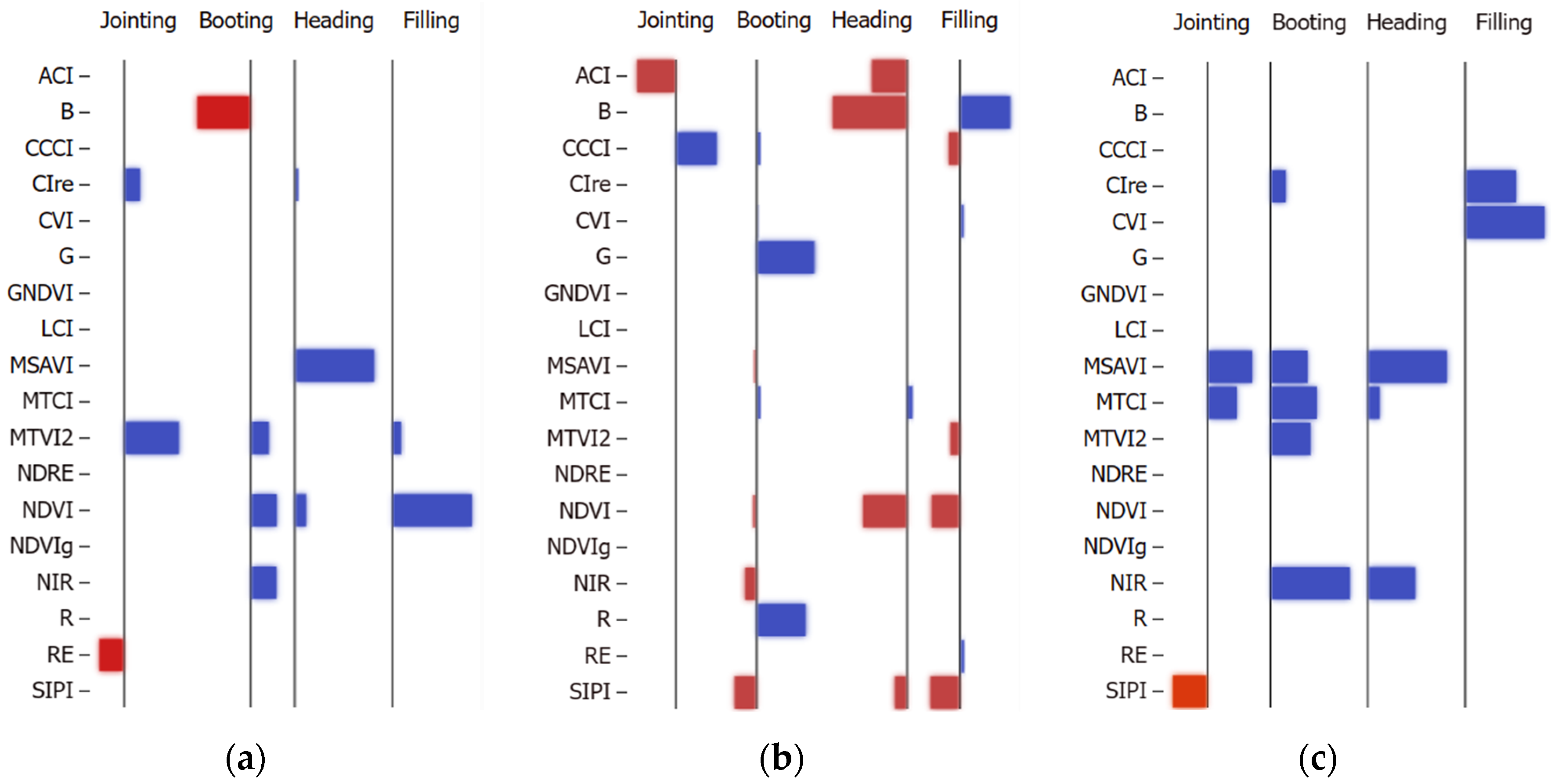
3.2.1. Feature Variable Selection
3.2.2. Model Accuracy Comparison
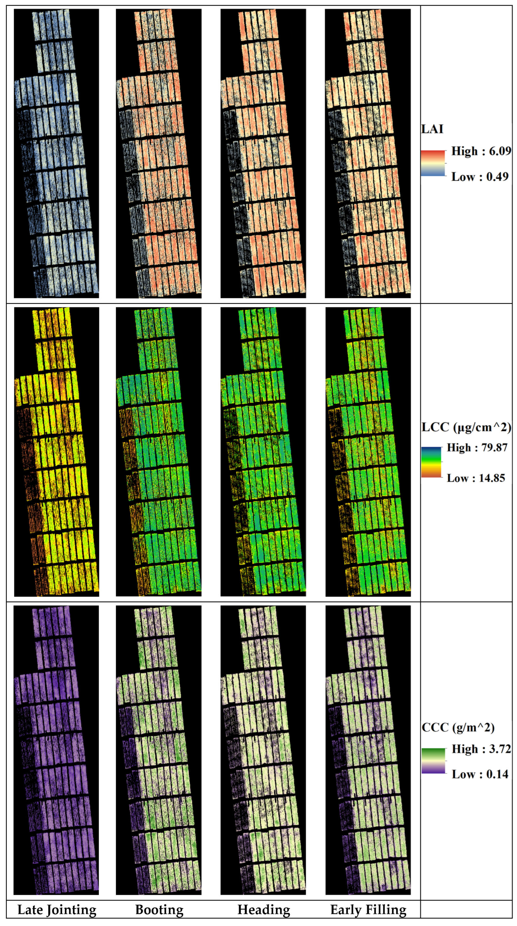
3.2.3. Winter Wheat Bio-Parameters Mapping
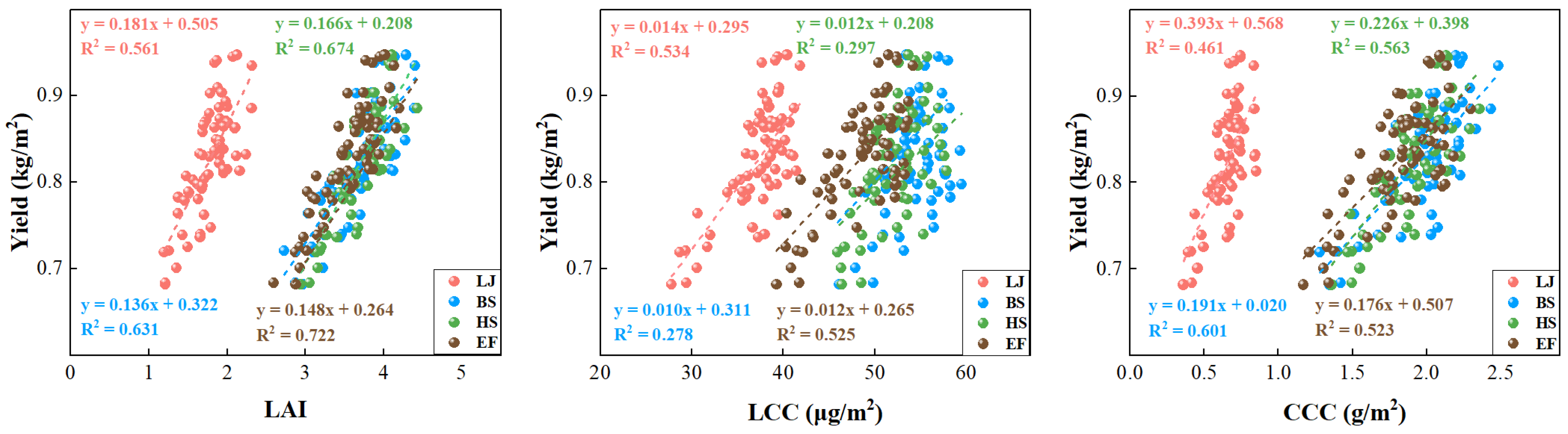
3.3. The Relationship between Winter Wheat Grain Yield and Biochemical Parameters
4. Discussion
4.1. Uncertainty of Observed Data
4.2. Comparison of Different Models
4.3. Effects of Crop Phenology on Bio-Parameters Estimation
5. Conclusions
Author Contributions
Funding
Data Availability Statement
Acknowledgments
Conflicts of Interest
References
- Lesk, C.; Rowhani, P.; Ramankutty, N. Influence of Extreme Weather Disasters on Global Crop Production. Nature 2016, 529, 84–87. [Google Scholar] [CrossRef]
- Vishwakarma, S.; Zhang, X.; Lyubchich, V. Wheat Trade Tends to Happen between Countries with Contrasting Extreme Weather Stress and Synchronous Yield Variation. Commun. Earth Environ. 2022, 3, 261. [Google Scholar] [CrossRef]
- Huang, J.; Sedano, F.; Huang, Y.; Ma, H.; Li, X.; Liang, S.; Tian, L.; Zhang, X.; Fan, J.; Wu, W. Assimilating a Synthetic Kalman Filter Leaf Area Index Series into the WOFOST Model to Improve Regional Winter Wheat Yield Estimation. Agric. For. Meteorol. 2016, 216, 188–202. [Google Scholar] [CrossRef]
- Huang, J.; Ma, H.; Su, W.; Zhang, X.; Huang, Y.; Fan, J.; Wu, W. Jointly Assimilating MODIS LAI and ET Products Into the SWAP Model for Winter Wheat Yield Estimation. IEEE J. Sel. Top. Appl. Earth Observ. Remote Sens. 2015, 8, 4060–4071. [Google Scholar] [CrossRef]
- Sus, O.; Heuer, M.W.; Meyers, T.P.; Williams, M. A Data Assimilation Framework for Constraining Upscaled Cropland Carbon Flux Seasonality and Biometry with MODIS. Biogeosciences 2013, 10, 2451–2466. [Google Scholar] [CrossRef]
- Schlemmer, M.; Gitelson, A.; Schepers, J.; Ferguson, R.; Peng, Y.; Shanahan, J.; Rundquist, D. Remote Estimation of Nitrogen and Chlorophyll Contents in Maize at Leaf and Canopy Levels. Int. J. Appl. Earth Obs. Geoinf. Int. 2013, 25, 47–54. [Google Scholar] [CrossRef]
- Gitelson, A.A.; Viña, A.; Verma, S.B.; Rundquist, D.C.; Arkebauer, T.J.; Keydan, G.; Leavitt, B.; Ciganda, V.; Burba, G.G.; Suyker, A.E. Relationship between Gross Primary Production and Chlorophyll Content in Crops: Implications for the Synoptic Monitoring of Vegetation Productivity. J. Geophys. Res. 2006, 111, 1–13. [Google Scholar] [CrossRef]
- Dorigo, W.A.; Zurita-Milla, R.; De Wit, A.J.W.; Brazile, J.; Singh, R.; Schaepman, M.E. A Review on Reflective Remote Sensing and Data Assimilation Techniques for Enhanced Agroecosystem Modeling. Int. J. Appl. Earth Obs. Geoinf. Int. 2007, 9, 165–193. [Google Scholar] [CrossRef]
- Wu, S.; Yang, P.; Ren, J.; Chen, Z.; Li, H. Regional Winter Wheat Yield Estimation Based on the WOFOST Model and a Novel VW-4DEnSRF Assimilation Algorithm. Remote Sens. Environ. 2021, 255, 112276. [Google Scholar] [CrossRef]
- Sanaeifar, A.; Yang, C.; De La Guardia, M.; Zhang, W.; Li, X.; He, Y. Proximal Hyperspectral Sensing of Abiotic Stresses in Plants. Sci. Total Environ. 2023, 861, 160652. [Google Scholar] [CrossRef]
- Wang, T.; Gao, M.; Cao, C.; You, J.; Zhang, X.; Shen, L. Winter Wheat Chlorophyll Content Retrieval Based on Machine Learning Using in Situ Hyperspectral Data. Comput. Electron. Agric. 2022, 193, 106728. [Google Scholar] [CrossRef]
- Zhang, Y.; Hui, J.; Qin, Q.; Sun, Y.; Zhang, T.; Sun, H.; Li, M. Transfer-Learning-Based Approach for Leaf Chlorophyll Content Estimation of Winter Wheat from Hyperspectral Data. Remote Sens. Environ. 2021, 267, 112724. [Google Scholar] [CrossRef]
- Sun, Q. Monitoring Maize Canopy Chlorophyll Density under Lodging Stress Based on UAV Hyperspectral Imagery. Comput. Electron. Agric. 2022, 193, 106671. [Google Scholar] [CrossRef]
- Longmire, A.R.; Poblete, T.; Hunt, J.R.; Chen, D.; Zarco-Tejada, P.J. Assessment of Crop Traits Retrieved from Airborne Hyperspectral and Thermal Remote Sensing Imagery to Predict Wheat Grain Protein Content. ISPRS-J. Photogramm. Remote Sens. 2022, 193, 284–298. [Google Scholar] [CrossRef]
- Zhu, W.; Sun, Z.; Yang, T.; Li, J.; Peng, J.; Zhu, K.; Li, S.; Gong, H.; Lyu, Y.; Li, B.; et al. Estimating Leaf Chlorophyll Content of Crops via Optimal Unmanned Aerial Vehicle Hyperspectral Data at Multi-Scales. Comput. Electron. Agric. 2020, 178, 105786. [Google Scholar] [CrossRef]
- Yu, K.; Lenz-Wiedemann, V.; Chen, X.; Bareth, G. Estimating Leaf Chlorophyll of Barley at Different Growth Stages Using Spectral Indices to Reduce Soil Background and Canopy Structure Effects. ISPRS-J. Photogramm. Remote Sens. 2014, 97, 58–77. [Google Scholar] [CrossRef]
- Zhang, S.; Zhao, G.; Lang, K.; Su, B.; Chen, X.; Xi, X.; Zhang, H. Integrated Satellite, Unmanned Aerial Vehicle (UAV) and Ground Inversion of the SPAD of Winter Wheat in the Reviving Stage. Sensors 2019, 19, 1485. [Google Scholar] [CrossRef]
- Cui, B.; Zhao, Q.; Huang, W.; Song, X.; Ye, H.; Zhou, X. Leaf Chlorophyll Content Retrieval of Wheat by Simulated RapidEye, Sentinel-2 and EnMAP Data. J. Integr. Agric. 2019, 18, 1230–1245. [Google Scholar] [CrossRef]
- Verrelst, J.; Rivera, J.P.; Gitelson, A.; Delegido, J.; Moreno, J.; Camps-Valls, G. Spectral Band Selection for Vegetation Properties Retrieval Using Gaussian Processes Regression. Int. J. Appl. Earth Obs. Geoinf. 2016, 52, 554–567. [Google Scholar] [CrossRef]
- Main, R.; Cho, M.A.; Mathieu, R.; O’Kennedy, M.M.; Ramoelo, A.; Koch, S. An Investigation into Robust Spectral Indices for Leaf Chlorophyll Estimation. ISPRS-J. Photogramm. Remote Sens. 2011, 66, 751–761. [Google Scholar] [CrossRef]
- Yue, J.; Yang, G.; Tian, Q.; Feng, H.; Xu, K.; Zhou, C. Estimate of Winter-Wheat above-Ground Biomass Based on UAV Ultrahigh-Ground-Resolution Image Textures and Vegetation Indices. ISPRS-J. Photogramm. Remote Sens. 2019, 150, 226–244. [Google Scholar] [CrossRef]
- Hunt, M.L.; Blackburn, G.A.; Carrasco, L.; Redhead, J.W.; Rowland, C.S. High Resolution Wheat Yield Mapping Using Sentinel-2. Remote Sens. Environ. 2019, 233, 111410. [Google Scholar] [CrossRef]
- Qi, H. Monitoring of Peanut Leaves Chlorophyll Content Based on Drone-Based Multispectral Image Feature Extraction. Comput. Electron. Agric. 2021, 187, 106292. [Google Scholar] [CrossRef]
- Zhang, L. Evaluating the Sensitivity of Water Stressed Maize Chlorophyll and Structure Based on UAV Derived Vegetation Indices. Comput. Electron. Agric. 2021, 187, 106292. [Google Scholar] [CrossRef]
- Wu, Q.; Zhang, Y.; Zhao, Z.; Xie, M.; Hou, D. Estimation of Relative Chlorophyll Content in Spring Wheat Based on Multi-Temporal UAV Remote Sensing. Agronomy 2023, 13, 211. [Google Scholar] [CrossRef]
- Zou, X.; Zhao, J.; Povey, M.J.W.; Holmes, M.; Hanpin, M. Variables Selection Methods in Near-Infrared Spectroscopy. Anal. Chim. Acta 2010, 667, 14–32. [Google Scholar]
- Chandrashekar, G.; Sahin, F. A Survey on Feature Selection Methods. Comput. Electr. Eng. 2014, 40, 16–28. [Google Scholar] [CrossRef]
- Uncu, Ö.; Türkşen, I.B. A Novel Feature Selection Approach: Combining Feature Wrappers and Filters. Inf. Sci. 2007, 177, 449–466. [Google Scholar] [CrossRef]
- Shafiee, S.; Lied, L.M.; Burud, I.; Dieseth, J.A.; Alsheikh, M.; Lillemo, M. Sequential Forward Selection and Support Vector Regression in Comparison to LASSO Regression for Spring Wheat Yield Prediction Based on UAV Imagery. Comput. Electron. Agric. 2021, 183, 106036. [Google Scholar] [CrossRef]
- Huang, X.; Guan, H.; Bo, L.; Xu, Z.; Mao, X. Hyperspectral Proximal Sensing of Leaf Chlorophyll Content of Spring Maize Based on a Hybrid of Physically Based Modelling and Ensemble Stacking. Comput. Electron. Agric. 2023, 208, 107745. [Google Scholar] [CrossRef]
- Han, S.; Zhao, Y.; Cheng, J.; Zhao, F.; Yang, H.; Feng, H.; Li, Z.; Ma, X.; Zhao, C.; Yang, G. Monitoring Key Wheat Growth Variables by Integrating Phenology and UAV Multispectral Imagery Data into Random Forest Model. Remote Sens. 2022, 14, 3723. [Google Scholar] [CrossRef]
- Wang, W.; Gao, X.; Cheng, Y.; Ren, Y.; Zhang, Z.; Wang, R.; Cao, J.; Geng, H. QTL Mapping of Leaf Area Index and Chlorophyll Content Based on UAV Remote Sensing in Wheat. Agriculture 2022, 12, 595. [Google Scholar] [CrossRef]
- Han, Y.; Tang, R.; Liao, Z.; Zhai, B.; Fan, J. A Novel Hybrid GOA-XGB Model for Estimating Wheat Aboveground Biomass Using UAV-Based Multispectral Vegetation Indices. Remote Sens. 2022, 14, 3506. [Google Scholar] [CrossRef]
- Wang, J.; Zhou, Q.; Shang, J.; Liu, C.; Zhuang, T.; Ding, J.; Xian, Y.; Zhao, L.; Wang, W.; Zhou, G.; et al. UAV- and Machine Learning-Based Retrieval of Wheat SPAD Values at the Overwintering Stage for Variety Screening. Remote Sens. 2021, 13, 5166. [Google Scholar] [CrossRef]
- Wang, W. Prediction of Chlorophyll Content in Multi-Temporal Winter Wheat Based on Multispectral and Machine Learning. Front. Plant Sci. 2022, 13, 896408. [Google Scholar] [CrossRef] [PubMed]
- Yin, Q.; Zhang, Y.; Li, W.; Wang, J.; Wang, W.; Ahmad, I.; Zhou, G.; Huo, Z. Estimation of Winter Wheat SPAD Values Based on UAV Multispectral Remote Sensing. Remote Sens. 2023, 15, 3595. [Google Scholar] [CrossRef]
- Zhang, C.; Xue, Y. Estimation of Biochemical Pigment Content in Poplar Leaves Using Proximal Multispectral Imaging and Regression Modeling Combined with Feature Selection. Sensors 2024, 24, 217. [Google Scholar] [CrossRef]
- Gruninger, J.H.; Ratkowski, A.J.; Hoke, M.L. The Sequential Maximum Angle Convex Cone (SMACC) Endmember Model. Proc. SPIE 2004, 5425, 1–14. [Google Scholar]
- Carter, G.A.; Cibula, W.G.; Miller, R.L. Narrow-Band Reflectance Imagery Compared with ThermalImagery for Early Detection of Plant Stress. J. Plant Physiol. 1996, 148, 515–522. [Google Scholar] [CrossRef]
- Barnes, E.M.; Clarke, T.R.; Richards, S.E. Coincident Detection of Crop Water Stress, Nitrogen Status, and Canopy Density Using Ground Based Multispectral Data. In Proceedings of the 5th International Conference on Precision Agriculture and Other Resource Management, Bloomington, MN, USA, 16–19 July 2000. [Google Scholar]
- Gitelson, A.A.; Viña, A.; Arkebauer, T.J.; Rundquist, D.C.; Keydan, G.; Leavitt, B. Remote Estimation of Leaf Area Index and Green Leaf Biomass in Maize Canopies. Geophys. Res. Lett. 2003, 30. [Google Scholar] [CrossRef]
- Datt, B.; McVicar, T.R.; Van Niel, T.G.; Jupp, D.L.B.; Pearlman, J.S. Preprocessing Eo-1 Hyperion Hyperspectral Data to Support the Application of Agricultural Indexes. IEEE Trans. Geosci. Remote Sens. 2003, 41, 1246–1259. [Google Scholar] [CrossRef]
- Gitelson, A.A.; Kaufman, Y.J.; Merzlyak, M.N. Use of a Green Channel in Remote Sensing of Global Vegetation from EOS-MODIS. Remote Sens. Environ. 1996, 58, 289–298. [Google Scholar] [CrossRef]
- Datt, B. Remote Sensing of Water Content in Eucalyptus Leaves. Aust. J. Bot. 1999, 47, 909. [Google Scholar] [CrossRef]
- Goel, N.S.; Qin, W. Influences of Canopy Architecture on Relationships between Various Vegetation Indices and LAI and Fpar: A Computer Simulation. Remote Sens. Rev. 1994, 10, 309–347. [Google Scholar] [CrossRef]
- Dash, J.; Curran, P.J. The MERIS Terrestrial Chlorophyll Index. Int. J. Remote Sens. 2004, 25, 5403–5413. [Google Scholar] [CrossRef]
- Haboudane, D. Hyperspectral Vegetation Indices and Novel Algorithms for Predicting Green LAI of Crop Canopies: Modeling and Validation in the Context of Precision Agriculture. Remote Sens. Environ. 2004, 90, 337–352. [Google Scholar] [CrossRef]
- Tucker, C.J.; Elgin, J.H.; McMurtrey, J.E.; Fan, C.J. Monitoring Corn and Soybean Crop Development with Hand-Held Radiometer Spectral Data. Remote Sens. Environ. 1979, 8, 237–248. [Google Scholar] [CrossRef]
- Blackburn, G.A. Spectral Indices for Estimating Photosynthetic Pigment Concentrations: A Test Using Senescent Tree Leaves. Int. J. Remote Sens. 1998, 19, 657–675. [Google Scholar] [CrossRef]
- Breiman, L. Random Forests. Mach. Learn. 2001, 45, 5–32. [Google Scholar] [CrossRef]
- CRAN-Package ‘mlr3fselect’ Instruction. Available online: http://ftp2.de.freebsd.org/pub/misc/cran/web/packages/mlr3fselect/mlr3fselect.pdf (accessed on 15 November 2023).
- Fonti, V. Feature Selection Using LASSO; VU Amsterdam: Amsterdam, The Netherlands, 2017; pp. 1–26. [Google Scholar]
- Wei, Z. Inversion of Winter Wheat Growth Parameters and Yield Under Different Water Treatments Based on UAV Multispectral Remote Sensing. Front. Plant Sci. 2021, 12, 609876. [Google Scholar]
- Dandrifosse, S.; Carlier, A.; Dumont, B.; Mercatoris, B. Registration and Fusion of Close-Range Multimodal Wheat Images in Field Conditions. Remote Sens. 2021, 13, 1380. [Google Scholar] [CrossRef]
- Li, H.; Zhao, C.; Huang, W.; Yang, G. Non-Uniform Vertical Nitrogen Distribution within Plant Canopy and Its Estimation by Remote Sensing: A Review. Field Crop. Res. 2013, 142, 75–84. [Google Scholar] [CrossRef]
- He, L.; Song, X.; Feng, W.; Guo, B.-B.; Zhang, Y.-S.; Wang, Y.-H.; Wang, C.-Y.; Guo, T.-C. Improved Remote Sensing of Leaf Nitrogen Concentration in Winter Wheat Using Multi-Angular Hyperspectral Data. Remote Sens. Environ. 2016, 174, 122–133. [Google Scholar] [CrossRef]
- Duan, D.; Zhao, C.; Li, Z.; Yang, G.; Yang, W. Estimating Total Leaf Nitrogen Concentration in Winter Wheat by Canopy Hyperspectral Data and Nitrogen Vertical Distribution. J. Integr. Agric. 2019, 18, 1562–1570. [Google Scholar] [CrossRef]
- Hu, P.; Chapman, S.C.; Jin, H.; Guo, Y.; Zheng, B. Comparison of Modelling Strategies to Estimate Phenotypic Values from an Unmanned Aerial Vehicle with Spectral and Temporal Vegetation Indexes. Remote Sens. 2021, 13, 2827. [Google Scholar] [CrossRef]
- Ganeva, D.; Roumenina, E.; Dimitrov, P.; Gikov, A.; Jelev, G.; Dyulgenova, B.; Valcheva, D.; Bozhanova, V. Remotely Sensed Phenotypic Traits for Heritability Estimates and Grain Yield Prediction of Barley Using Multispectral Imaging from UAVs. Sensors 2023, 23, 5008. [Google Scholar] [CrossRef] [PubMed]
- Li, W.; Li, D.; Liu, S.; Baret, F.; Ma, Z.; He, C.; Warner, T.A.; Guo, C.; Cheng, T.; Zhu, Y.; et al. RSARE: A Physically-Based Vegetation Index for Estimating Wheat Green LAI to Mitigate the Impact of Leaf Chlorophyll Content and Residue-Soil Background. ISPRS-J. Photogramm. Remote Sens. 2023, 200, 138–152. [Google Scholar] [CrossRef]
- Duan, B.; Fang, S.; Zhu, R.; Wu, X.; Wang, S.; Gong, Y.; Peng, Y. Remote Estimation of Rice Yield With Unmanned Aerial Vehicle (UAV) Data and Spectral Mixture Analysis. Front. Plant Sci. 2019, 10, 204. [Google Scholar] [CrossRef] [PubMed]


| Ground and UAV Measurement Data (2023) | Growth Stage Description | Abbreviation |
|---|---|---|
| 31 March | Late Jointing Stage (DAS 172) | LJ |
| 12 April | Booting Stage (DAS 184) | BS |
| 26 April | Heading Stage (DAS 198) | HS |
| 12 May | Early Filling Stage (DAS 214) | FS |
| Parameters | Parameter Value |
|---|---|
| Flight altitude | 50 m |
| Flight Speed | 3.8 m/s |
| Heading overlap ratio | 75% |
| Collateral overlap ratio | 80% |
| Ground Sampling Distance | 3 cm |
| Variable | Abbreviation | Formulation | Reference |
|---|---|---|---|
| Blue band | B | — | |
| Green band | G | — | |
| Red band | R | — | |
| Red edge band | RE | — | |
| NIR band | NIR | — | |
| Agriculture Chlorophyll Index | ACI | Green/NIR | [39] |
| Canopy Chlorophyll Content Index | CCCI | NDRE/NDVI | [40] |
| Chlorophyll Index using Red Edge Reflectance | CIred-edge | (NIR/Edge) − 1 | [41] |
| Chlorophyll Vegetation Index | CVI | NIR × (Red/Blue2) | [42] |
| Green Normalized Difference Vegetation Index | GNDVI | (NIR − Green)/(NIR + Green) | [43] |
| Leaf Chlorophyll Index | LCI | (NIR − Edge)/(NIR + Red) | [44] |
| Modified Soil Adjusted Vegetation Index | MSAVI | [45] | |
| MERIS Terrestrial Chlorophyll Index | MTCI | (NIR − Edge)/(Edge − Red) | [46] |
| Modified Triangular Vegetation Index 2 | MTVI2 | [47] | |
| Normalized Difference Red Edge Index | NDRE | (NIR − Edge)/(NIR + Edge) | [40] |
| Normalized Difference Vegetation Index | NDVI | (NIR − Red)/(NIR + Red) | [48] |
| Green NDVI | NDVIg | (Edge − Green)/(Edge + Green) | [43] |
| Structure Insensitive Pigment Index | SIPI | (NIR − Blue)/(NIR − Red) | [49] |
| Growth Stage | Parameter | Samples | Min | Mean | Max | S·D |
|---|---|---|---|---|---|---|
| Jointing | LAI | 40 | 0.70 | 1.88 | 3.37 | 0.81 |
| LCC (μg/cm2) | 15.40 | 35.83 | 51.68 | 11.42 | ||
| CCC (g/m2) | 0.12 | 0.70 | 1.42 | 0.44 | ||
| Booting | LAI | 46 | 1.47 | 3.55 | 5.30 | 1.24 |
| LCC (μg/cm2) | 24.47 | 51.70 | 66.65 | 11.48 | ||
| CCC (g/m2) | 0.36 | 1.84 | 3.05 | 0.84 | ||
| Heading | LAI | 52 | 1.57 | 3.46 | 5.65 | 1.04 |
| LCC (μg/cm2) | 28.20 | 52.45 | 66.72 | 10.01 | ||
| CCC (g/m2) | 0.42 | 1.74 | 3.25 | 0.70 | ||
| Filling | LAI | 56 | 1.45 | 3.57 | 5.82 | 1.11 |
| LCC (μg/cm2) | 20.44 | 50.41 | 70.08 | 13.32 | ||
| CCC (g/m2) | 0.30 | 1.75 | 2.91 | 0.76 | ||
| All Stages | LAI | 194 | 0.70 | 3.26 | 5.82 | 1.23 |
| LCC (μg/cm2) | 15.40 | 48.93 | 70.08 | 12.98 | ||
| CCC (g/m2) | 0.12 | 1.60 | 3.25 | 0.82 |
| Variables | Late Jointing | Booting | Heading | Early Filling | ||||||||
|---|---|---|---|---|---|---|---|---|---|---|---|---|
| LASSO | RF | SFS | LASSO | RF | SFS | LASSO | RF | SFS | LASSO | RF | SFS | |
| B | √ | √ | √ | √ | √ | |||||||
| G | √ | √ | ||||||||||
| R | √ | √ | √ | |||||||||
| RE | √ | √ | √ | √ | ||||||||
| NIR | √ | |||||||||||
| ACI | √ | √ | √ | |||||||||
| CCCI | ||||||||||||
| CIre | √ | √ | √ | |||||||||
| CVI | √ | |||||||||||
| GNDVI | √ | √ | ||||||||||
| LCI | √ | √ | ||||||||||
| MSAVI | √ | √ | ||||||||||
| MTCI | ||||||||||||
| MTVI2 | √ | √ | √ | √ | √ | √ | √ | √ | ||||
| NDRE | ||||||||||||
| NDVI | √ | √ | √ | √ | √ | |||||||
| NDVIg | √ | |||||||||||
| SIPI | √ | √ | √ | √ | √ | |||||||
| Variables | Jointing | Booting | Heading | Filling | ||||||||
|---|---|---|---|---|---|---|---|---|---|---|---|---|
| LASSO | RF | SFS | LASSO | RF | SFS | LASSO | RF | SFS | LASSO | RF | SFS | |
| B | √ | √ | √ | √ | ||||||||
| G | √ | √ | ||||||||||
| R | √ | |||||||||||
| RE | √ | √ | √ | |||||||||
| NIR | √ | √ | ||||||||||
| ACI | √ | √ | √ | |||||||||
| CCCI | √ | √ | √ | √ | √ | √ | √ | √ | √ | |||
| CIre | √ | √ | ||||||||||
| CVI | √ | √ | √ | |||||||||
| GNDVI | ||||||||||||
| LCI | √ | √ | ||||||||||
| MSAVI | √ | √ | √ | |||||||||
| MTCI | √ | √ | √ | √ | ||||||||
| MTVI2 | √ | √ | ||||||||||
| NDRE | √ | |||||||||||
| NDVI | √ | √ | √ | √ | ||||||||
| NDVIg | √ | |||||||||||
| SIPI | √ | √ | √ | √ | √ | √ | ||||||
| Variables | Jointing | Booting | Heading | Filling | ||||||||
|---|---|---|---|---|---|---|---|---|---|---|---|---|
| LASSO | RF | SFS | LASSO | RF | SFS | LASSO | RF | SFS | LASSO | RF | SFS | |
| B | √ | √ | √ | |||||||||
| G | ||||||||||||
| R | √ | √ | ||||||||||
| RE | √ | √ | ||||||||||
| NIR | √ | √ | √ | √ | ||||||||
| ACI | √ | √ | ||||||||||
| CCCI | ||||||||||||
| CIre | √ | √ | √ | √ | √ | |||||||
| CVI | √ | √ | √ | √ | ||||||||
| GNDVI | √ | √ | √ | |||||||||
| LCI | √ | |||||||||||
| MSAVI | √ | √ | √ | √ | ||||||||
| MTCI | √ | √ | √ | √ | √ | |||||||
| MTVI2 | √ | |||||||||||
| NDRE | ||||||||||||
| NDVI | ||||||||||||
| NDVIg | √ | |||||||||||
| SIPI | √ | √ | √ | |||||||||
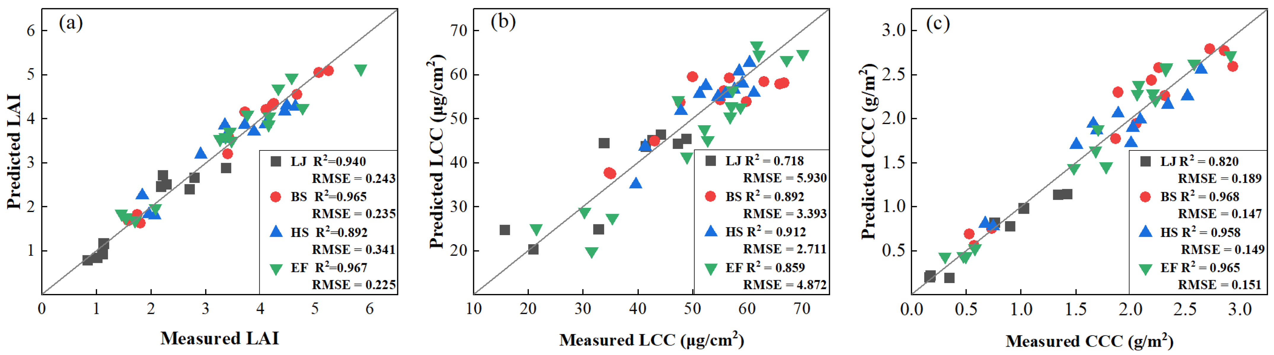
| Late Jointing | Model | LAI | LCC | CCC | |||||||||
| Training set | Test set | Training set | Test set | Training set | Test set | ||||||||
| RMSE | RPD | RMSE | RPD | RMSE (μg/cm2) | RPD | RMSE (μg/cm2) | RPD | RMSE (g/m2) | RPD | RMSE (g/m2) | RPD | ||
| LASSO | 0.204 | 4.417 | 0.318 | 2.502 | 5.224 | 2.022 | 5.993 | 1.771 | 0.132 | 3.432 | 0.114 | 3.503 | |
| RFR | 0.108 | 7.111 | 0.267 | 2.439 | 1.992 | 5.588 | 6.405 | 1.461 | 0.056 | 7.247 | 0.113 | 3.101 | |
| SFS-SVR | 0.201 | 4.129 | 0.243 | 3.184 | 5.032 | 1.876 | 5.93 | 1.786 | 0.076 | 5.738 | 0.189 | 2.249 | |
| Booting | Model | LAI | LCC | CCC | |||||||||
| Training set | Test set | Training set | Test set | Training set | Test set | ||||||||
| RMSE | RPD | RMSE | RPD | RMSE (μg/cm2) | RPD | RMSE (μg/cm2) | RPD | RMSE (g/m2) | RPD | RMSE (g/m2) | RPD | ||
| LASSO | 0.25 | 4.650 | 0.301 | 4.392 | 3.34 | 3.396 | 5.201 | 1.501 | 0.141 | 5.701 | 0.218 | 3.837 | |
| RFR | 0.094 | 14.699 | 0.403 | 3.543 | 3.127 | 3.933 | 5.097 | 2.071 | 0.098 | 9.362 | 0.227 | 4.069 | |
| SFS-SVR | 0.255 | 4.702 | 0.235 | 4.856 | 3.477 | 2.831 | 3.393 | 2.530 | 0.140 | 5.531 | 0.147 | 5.279 | |
| Heading | Model | LAI | LCC | CCC | |||||||||
| Training set | Test set | Training set | Test set | Training set | Test set | ||||||||
| RMSE | RPD | RMSE | RPD | RMSE (μg/cm2) | RPD | RMSE (μg/cm2) | RPD | RMSE (g/m2) | RPD | RMSE (g/m2) | RPD | ||
| LASSO | 0.261 | 3.904 | 0.314 | 2.795 | 4.349 | 1.562 | 3.893 | 1.818 | 0.162 | 3.349 | 0.151 | 3.383 | |
| RFR | 0.124 | 9.954 | 0.377 | 2.671 | 2.408 | 3.962 | 4.219 | 2.186 | 0.073 | 11.404 | 0.300 | 2.290 | |
| SFS-SVR | 0.250 | 3.760 | 0.341 | 2.449 | 4.277 | 1.804 | 2.711 | 2.872 | 0.125 | 5.190 | 0.149 | 4.460 | |
| Early Filling | Model | LAI | LCC | CCC | |||||||||
| Training set | Test set | Training set | Test set | Training set | Test set | ||||||||
| RMSE | RPD | RMSE | RPD | RMSE (μg/cm2) | RPD | RMSE (μg/cm2) | RPD | RMSE (g/m2) | RPD | RMSE (g/m2) | RPD | ||
| LASSO | 0.255 | 3.840 | 0.404 | 2.852 | 4.336 | 2.773 | 4.671 | 2.565 | 0.166 | 4.226 | 0.184 | 3.603 | |
| RFR | 0.126 | 10.277 | 0.337 | 3.987 | 2.236 | 6.257 | 6.784 | 1.736 | 0.086 | 10.241 | 0.209 | 4.242 | |
| SFS-SVR | 0.229 | 4.956 | 0.225 | 4.905 | 5.022 | 2.524 | 4.872 | 2.222 | 0.160 | 4.906 | 0.151 | 4.884 | |
Disclaimer/Publisher’s Note: The statements, opinions and data contained in all publications are solely those of the individual author(s) and contributor(s) and not of MDPI and/or the editor(s). MDPI and/or the editor(s) disclaim responsibility for any injury to people or property resulting from any ideas, methods, instructions or products referred to in the content. |
© 2024 by the authors. Licensee MDPI, Basel, Switzerland. This article is an open access article distributed under the terms and conditions of the Creative Commons Attribution (CC BY) license (https://creativecommons.org/licenses/by/4.0/).
Share and Cite
Zhang, C.; Yi, Y.; Wang, L.; Zhang, X.; Chen, S.; Su, Z.; Zhang, S.; Xue, Y. Estimation of the Bio-Parameters of Winter Wheat by Combining Feature Selection with Machine Learning Using Multi-Temporal Unmanned Aerial Vehicle Multispectral Images. Remote Sens. 2024, 16, 469. https://doi.org/10.3390/rs16030469
Zhang C, Yi Y, Wang L, Zhang X, Chen S, Su Z, Zhang S, Xue Y. Estimation of the Bio-Parameters of Winter Wheat by Combining Feature Selection with Machine Learning Using Multi-Temporal Unmanned Aerial Vehicle Multispectral Images. Remote Sensing. 2024; 16(3):469. https://doi.org/10.3390/rs16030469
Chicago/Turabian StyleZhang, Changsai, Yuan Yi, Lijuan Wang, Xuewei Zhang, Shuo Chen, Zaixing Su, Shuxia Zhang, and Yong Xue. 2024. "Estimation of the Bio-Parameters of Winter Wheat by Combining Feature Selection with Machine Learning Using Multi-Temporal Unmanned Aerial Vehicle Multispectral Images" Remote Sensing 16, no. 3: 469. https://doi.org/10.3390/rs16030469