


Sea Ice Detection Method Using the Dependence of the Radar Cross-Section on the Incidence Angle

Institute of Applied Physics, Russian Academy of Sciences, 603950 Nizhny Novgorod, Russia
*
Author to whom correspondence should be addressed.
Remote Sens. 2024, 16(5), 859; https://doi.org/10.3390/rs16050859
Submission received: 22 January 2024
/
Revised: 22 February 2024
/
Accepted: 26 February 2024
/
Published: 29 February 2024
(This article belongs to the Special Issue Recent Advances in Sea Ice Research Using Satellite Data)
Abstract
:The method for sea ice detection using the data from the Dual-frequency Precipitation Radar (DPR) onboard the Global Precipitation Measurement (GPM) satellite data is suggested. The approach is based on the analysis of the shape of normalized radar cross-section dependence on the incidence angle. The coefficient of kurtosis of surface slopes probability density function is introduced as a parameter to distinguish between open water and ice cover. The approach was validated using the data on sea ice concentration from the AMSR-2 radiometer in the Antarctic region.
1. Introduction
The analysis of sea surface slope statistics originated from the study conducted by Cox and Munk [1]. They demonstrated, using photographs of the sun’s glitter, that sea surface slopes follow a Gram–Charlier distribution, which closely resembles a normal distribution. Furthermore, the relationship between the parameters of the sea surface slope probability density function and wind speed was investigated. These findings were later revisited and validated in a subsequent study in [2].
In [3], the third and fourth statistical moments of the distribution were obtained in the experiment with the optical scanners.
In [4], Ku-band microwave radar data were used to obtain quasi-Gaussian, two-dimensional slope PDF. The data from the Dual-frequency Precipitation Radar (DPR) onboard the Global Precipitation Measurement (GPM) satellite were used. All the parameters of the slope PDF were inverted with a non-linear least square fit of the backscattering coefficients. The empirical formulae relating the statistical parameters of the quasi-Gaussian sea slope PDF with wind speed were established.
However, flat water surface slopes do not follow quasi-Gaussian statistics. There is a range of states between the flat sea surface and the surface with developed waves. Wind conditions influence sea surface slope behavior. Ice cover also modifies it.
The surface covered with ice is generally flatter than sea waves. Thus, changes in the surface slope statistics can serve as the criterion for sea ice detection. In this paper, the coefficient of kurtosis of surface slope PDF is considered to be a parameter, defining the proximity of slope statistics to Gaussian. The data of DPR Ku-band radar at low incidence angles are used to study the coefficient of kurtosis depending on the surface type: open water and sea ice.
Sea ice detection at low incidence angles is a new and challenging task for remote sensing society. Several works were devoted to sea ice detection using normalized radar cross-section (NRCS) value measured by Sea Wave Investigation and Measurement (SWIM) radar onboard Chinese-French Oceanography Satellite (CFOSAT) and DPR [5,6,7]. SWIM is the Ku-band radar that has beams with incidence angles from to . DPR consists of the Ku-and Ka-band radars operating at incidence angles below .
In [5], sea ice type in the Arctic region is determined based on several features of the reflected pulse of SWIM radar. The method based on the Bayesian approach, presented in [6], using SWIM radar data on NRCS, revealed good accuracy for incidence angles below 6 degrees. At the same time, a simple classification method based on unsupervised clustering has shown good performance at 4–18 degrees [7]. The problems of sea ice detection using only the data on NRCS for unsupervised clustering occur at incidence angles below . The alternative approach based on the information about surface slope statistics is considered in the present paper.
The paper is organized as follows. In Section 2, the dataset is described. Section 3 presents the method to calculate the coefficient of kurtosis and the statistics of this parameter, and after that, the method for sea ice detection is discussed. Section 4 presents the results for sea ice detection, and the results are summarized in the conclusion.
2. Data
The GPM satellite was launched in February 2014, carrying five instruments, including the DPR and radiometer GPM Microwave Imager (GMI). The satellite ground track is confined between 65°S and 65°N. The DPR is a Ku- and Ka-band pulsed radar with horizontal polarization. The DPR antenna scans perpendicularly to the flight direction. The scanning angle varies from −17° to +17°, with 49 beam positions separated by 0.71°. The local incidence angle depends on the shape of the Earth. Maximum local incidence angle is approximately , and spatial resolution is about 5 km. The GPM data contains a land mask and rain flag for each resolution element. The data with precipitation were excluded from consideration, as well as all the scans containing the data over land. Auxiliary data on near-surface wind speed at 10 m height () resampled to DPR resolution elements were used. They are the Japanese Global Analysis model data (GANAL) used to provide atmospheric environmental conditions. The data are resampled and distributed by the DPR team as a complementary dataset and are stored in the GPM/DPR ENV product.
In this work, Ku-band radar data on normalized cross-section (NRCS) for July 2018 over Antarctica are used for latitudes south of 50°S.
Sea ice concentration (SIC) from AMSR-2 data were used for validation. The data are available on the Bremen University website. SIC is obtained according to the ASI algorithm [8]. The data contain gridded daily SIC products with 6.25 km resolution. The values of SIC were resampled to DPR resolution elements. The samples with SIC are labeled as “ice”, and those with SIC < 0.15 are labeled as “water”. The value 0.15 was chosen as a typical threshold for ice/ocean discrimination [9].
The example of a DPR swath over Antarctic ice is presented in Figure 1. It should be noted that the relationship between NRCS and incidence angle varies based on the underlying surface, whether it is water or ice.
3. Sea Ice Detection Method
3.1. Coefficient of Kurtosis Calculation
The backscatter of microwaves by the sea surface at low incidence angles is described within the framework of geometrical optics approximation. According to this approximation, NRCS is proportional to the slope probability density function (PDF) along the direction of scanning [10], and the dependence of NRCS on incidence angle is as follows:
where is the effective reflection coefficient. It was shown [10] that surface slopes PDF for sea surface is close to normal distribution.
where are mean square slopes along and across scanning direction, respectively. This approximation is valid for incidence angles within the range according to [11].
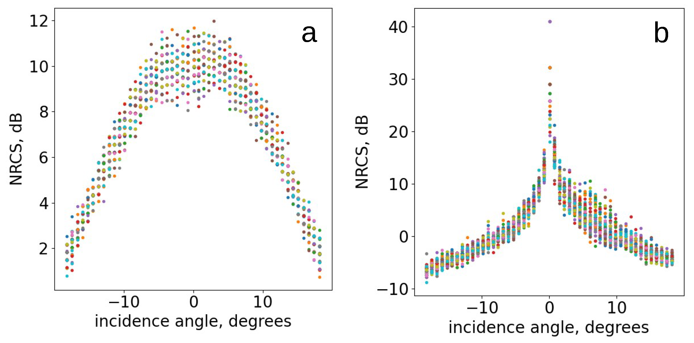
From Figure 2, the peculiarity of for sea ice is the narrow peak at . The presence of this peak can be explained by the fact that for almost flat ice cover, there are much fewer facets tilted from the horizontal than for sea waves. For the water surface, has a wide peak. Thus, it is assumed that surface slope PDFs for ice and sea waves obtained from are different.
It is known that the coefficient of kurtosis describes the sharpness of a peak of the curve of PDF and the steepness of slopes of the distribution tails. The sharper the curve peak near the center of the distribution, the greater the value of the coefficient of kurtosis.
The kurtosis for PDF is calculated as follows [12]
where and are the central statistical moments of PDF. The equation for from DPR data is obtained in the Appendix A for the case of discrete measurements, and here it is given in a final form
where is an incidence angle of DPR beam, is NRCS measured at .
Each half of the swath is considered separately. First the part of the swath where is augmented symmetrically, so that . The coefficient of kurtosis is calculated for this complemented swath, originating from the half with . The obtained is assigned to the pixels of the corresponding half of the scan. The same procedure is performed for another half with .
In Figure 3, the example of data processing is presented. The part of the swath shown in Figure 1 is considered. Raw data of the swath for all 49 beams over Antarctic ice is shown in the top figure. In the middle, sea ice concentration within the swath is presented, and at the bottom, the coefficient of kurtosis for both parts of the swath is shown. The value of the kurtosis coefficient is assigned to each resolution element of the half-scan for the calculation of which data were used. The coefficient of kurtosis for the present dataset varies between −1.9 and 3500. Thus, here and after the value equal to is plotted. For the case in Figure 3, high coefficients of kurtosis correspond to ice cover, and low values occur over the sea surface.
In the middle part, dashed and solid lines correspond to the incidence angles and . The cuts along these lines are presented in Figure 4. The upper half of Figure 3 contains a longer strip of ice. Between scans 100 and 150, the lower half of the DPR swath is over water, and the upper part is over ice. The kurtosis coefficient dependence corresponding to the upper half is shown in the dashed line in Figure 4 and is located higher than the dependence in the solid line for the water surface. This example exhibits the improvement of resolution when the two swath halves are considered separately.
The value of for water surface is close to zero and slightly below zero, while for Gaussian statistics, it equals zero. A possible reason is that this coefficient is calculated using a limited range of incidence angles in discrete points. The value of over the sea ice surface is much greater than zero and exhibits sharp spikes along the cut reaching several hundred.
3.2. Sea Ice Detection Method
The coefficient of kurtosis was calculated as described above for all the DPR data for July 2018 at the latitudes south of 50°S using NRCS at incidence angles below .
In the present work for sea ice detection, only the areas corresponding to the central part of the swath (incidence angles below ) are considered. This part of the swath is located between grey lines in Figure 3. The part of the swath is confined in such a way as to study the performance of sea ice detection in the area where clustering based on NRCS value from [7] exhibits weak results. Another reason is the limitation of resolution element size along the scanning direction.
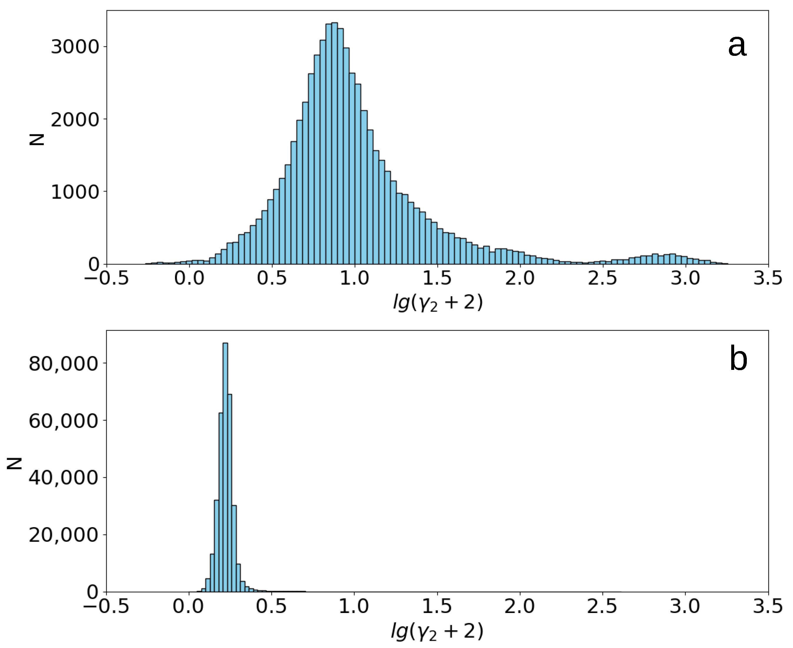
First, among the entire dataset, only the scans, totally located over water and totally located over ice, were selected. It is performed to study the statistics of for simple cases when only one type of underlying surface is presented. For these data, the histograms for are shown in Figure 5.
The maximum distribution for the water surface is at , and for sea ice, the maximum of the histogram is at . The histogram for sea ice has a secondary peak at .
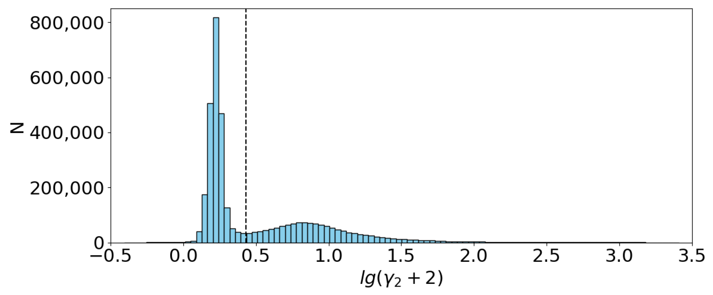
In Figure 6, the entire dataset of for July 2018 around Antarctica is presented. In this case, unlike the previous figure, the half-scans with different types of surfaces are also contained in the dataset. From Figure 6, it follows that the two peaks are nevertheless well separated. The thresholding method can be used for water-ice classification. In this paper, the unsupervised method is considered. It means that the threshold is obtained using the dataset of interest. Preliminary training is not required. The two options are considered.
The first option is to obtain the threshold using the unsupervised clustering method K-means. The threshold, in this case, for equals to 2.89. The second option is to obtain corresponding to the minimum between the two peaks of the histogram in Figure 6. In this case, the threshold for equals to 0.69.
The F-score metric was calculated to evaluate the efficiency of classification and choose the optimal thresholding method.
where true positive ( ) refers to the number of samples accurately identified as ice, while true negative () is the number of samples accurately identified as water. False positive () represents the number of samples mistakenly labeled as ice, and false negative () is the number of samples mistakenly labeled as water. When we use the terms “accurately” and “mistakenly”, we are referring to the SIC data as the ground truth.
In the case of , , while in the case of , . Thus, the second option for selecting the threshold value of is preferred. The subsequent results are given for this method.
To conclude, the classification of surface type includes the following steps:
- Calculating the coefficient of kurtosis for each symmetrically complemented half of the swath, the value of the coefficient is assigned to each element of the half-scan.
- Unsupervised classification is performed. The histogram of for the entire dataset is obtained. The minimum between the two highest peaks of the histogram corresponds to the threshold value , separating “ice” and “water” classes.
The elements with are labeled as ice, the remaining elements with are labeled as water.
4. Results and Discussion
Classification of the sea surface type was performed as described above. High values of the coefficient of kurtosis correspond to the flat surface. It can be an ice surface or a calm sea. The dataset on wind speed was used to select the resolution elements with wind speed below 3 m/s and to evaluate the number of false positives related to these conditions.
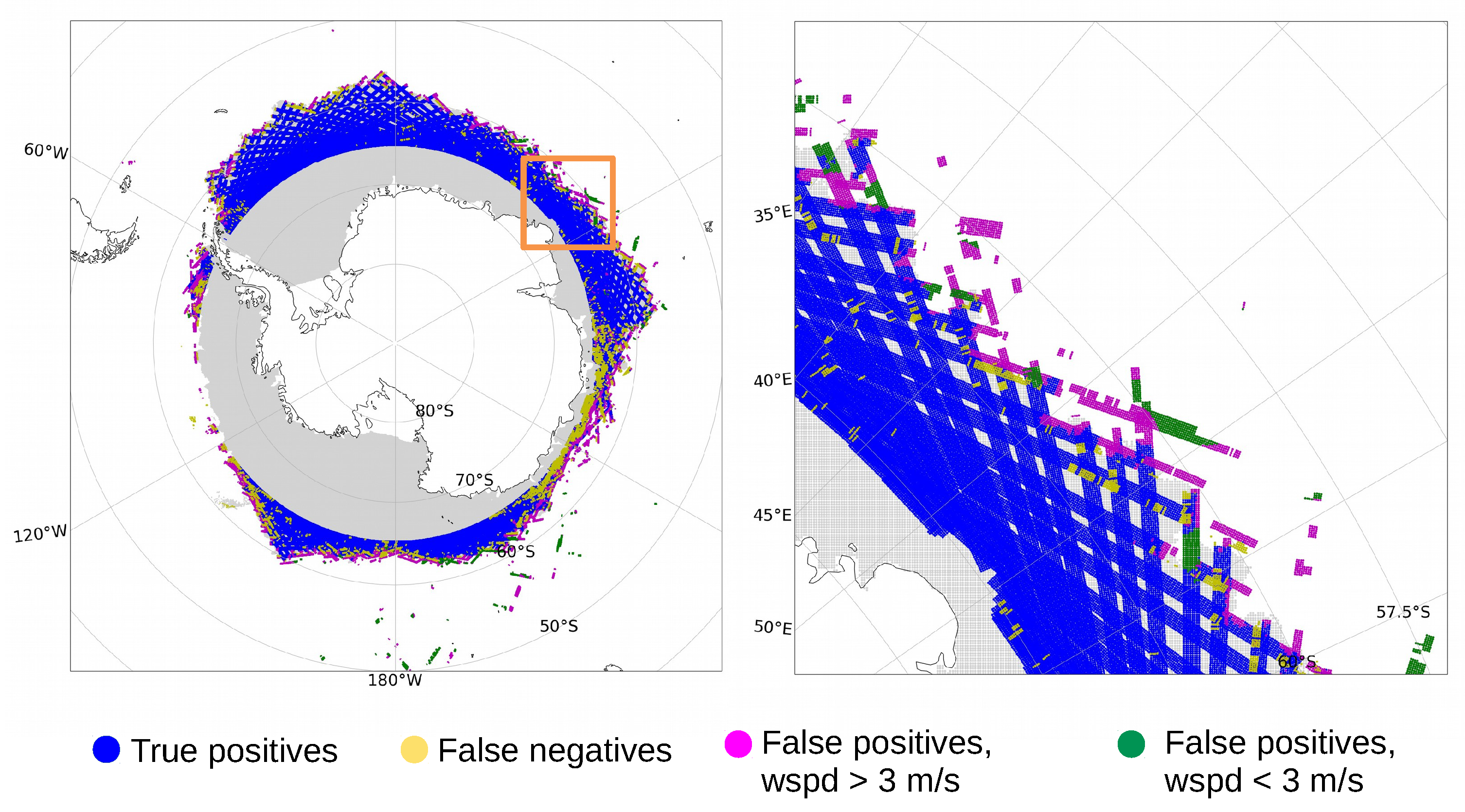
The results for the last week of July 2018 are presented in Figure 7. The resolution elements correctly defined as ice are marked in blue, and the elements erroneously defined as water are marked in yellow. The elements erroneously marked as ice at m/s are shown in magenta, and at low wind speed m/s are marked in green. Most of the elements, erroneously marked as ice, located far from the ice edge in the ocean, correspond to low wind speed cases. Ice cover with is shown in grey for July 27.
For this dataset, , , , , and among these samples, at m/s.
The obvious drawback of the presented method for sea ice detection using DPR data is the fact that measurements at different incidence angles are performed in a wide swath. Thus, the single value of the coefficient of kurtosis characterizes a broad area where the type of the surface may vary. This method performs well at large ice fields and has problems near the ice edge. Also, the data from the scans that cover the coast are neglected.
The advantage of the approach is that no precise calibration of the radar is required according to Equation (A8), unlike the methods based on the value of NRCS [6,7]. In the present work, unsupervised clustering was applied. It means that the method can be adapted for different geographic areas and seasons.
The performance of the method was evaluated for the central part of the swath, corresponding to the incidence angles below . The half of the central part of the scan, with a constant coefficient of kurtosis, can be called the resolution element. Its size is 25 km along the scanning direction and 5 km along the flight direction.
The performance of the algorithm is good, F-score = 0.93. While the unsupervised method for ice detection in [7] performs worse for this part of the swath (F-score < 0.9). Furthermore, the two approaches can be combined.
5. Conclusions
In the present work, a new method for sea ice detection using radar data at low incidence angles was developed. The approach is focused on the dependence of NRCS on incidence angle based on Ku-band DPR data. Within the frameworks of quasispecular approximation, a method to calculate the coefficient of kurtosis for surface slopes probability density function (PDF) was developed from the dependence of NRCS on incidence angle. It was shown that this coefficient can serve as a parameter to differentiate between surfaces with Gaussian slope statistics and flat surfaces. DPR data for July 2018 in the Antarctic area were used.
The analysis revealed a distinct separation between the histograms of the coefficient of kurtosis for ice-covered and open-water surfaces. Consequently, unsupervised clustering was used to categorize the two surface types. Low values of the coefficient of kurtosis correspond to a wavy water surface, and high values of kurtosis indicate ice-covered regions. The threshold value of the coefficient of kurtosis is selected as a position of the minimum between the two main peaks of the histogram. The case of a relatively flat water surface, free of ice, is considered separately. It was shown that the fraction of such calm sea regions where sea ice is erroneously detected is not large.
Sea ice concentration data obtained from AMSR-2 measurements were used as ground truth. The performance of the algorithm was evaluated for the central part of the swath for incidence angles below . In this area, sea ice detection based on the value of NRCS from [7] suffers problems. The new approach revealed good performance for the considered dataset F-score equal to 0.93. Thus, the new approach can be used to complement the sea ice detection method described in [7]. Moreover, the idea of using the information on surface slope statistics can be applied to sea ice detection using SWIM radar data.
Author Contributions
Conceptualization, M.P.; methodology, M.P.; software, M.P.; validation, M.P.; data curation, M.P.; writing—original draft preparation, M.P.; writing—review and editing, M.P. and V.K.; visualization, M.P. All authors have read and agreed to the published version of the manuscript.
Funding
The study was carried out at the expense of a grant from the Russian Science Foundation (project No. 23-77-10064).
Data Availability Statement
DPR data were downloaded from https://storm.pps.eosdis.nasa.gov, accessed on 5 September 2022, SIC data were downloaded from https://seaice.uni-bremen.de/databrowser, accessed on 15 March 2023.
Acknowledgments
The author thanks Alexandr Shikov, Kirill Ponur, Maria Ryabkova, and Yury Titchenko for their discussion and valuable comments.
Conflicts of Interest
The authors declare no conflicts of interest.
Abbreviations
The following abbreviations are used in this manuscript:
| AMSR-2 | Advanced Microwave Scanning Radiometer 2 |
| CFOSAT | Chinese-French Oceanography Satellite |
| DPR | Dual-Frequency Precipitation Radar |
| FN | False Negative |
| FP | False Positive |
| GANAL | Japanese Global Analysis model data |
| GPM | Global Precipitation Measurements |
| NRCS | Normalized Radar Cross-Section |
| SIC | Sea Ice Concentration |
| SWIM | Sea Wave Investigation and Measurement |
| TN | True Negative |
| TP | True Positive |
Appendix A
The equation for NRCS depending on the incidence angle is as follows:
where P is slope PDF, A stands for for brevity. Statistical moments of PDF P, in theory, are calculated as follows:
and is the expected value of x
From (1A), the slope PDF is retrieved for each antenna beam
Due to the fact that cumulative distribution function at equals to 1,
Measurements at incidence angles above are not used. However, at such incidence angles, takes low values, and integral from to can be neglected. Thus
If we consider the part of the scan for , . From this equation, the coefficient A is obtained.
References
- Cox, C.; Munk, W. Measurement of the roughness of the sea surface from photographs of the sun’s glitter. J. Opt. Soc. Am. 1954, 44, 838–850. [Google Scholar] [CrossRef]
- Bréon, F.M.; Henriot, N. Spaceborne observations of ocean glint reflectance and modeling of wave slope distributions. J. Geophys. Res. Ocean. 2006, 111, C06005. [Google Scholar] [CrossRef]
- Zapevalov, A. Determination of the Statistical Moments of Sea-Surface Slopes by Optical Scanners. Atmos. Ocean. Opt. 2018, 31, 91–95. [Google Scholar] [CrossRef]
- Chen, P.; Zheng, G.; Hauser, D.; Xu, F. Quasi-Gaussian probability density function of sea wave slopes from near nadir Ku-band radar observations. Remote Sens. Environ. 2018, 217, 86–100. [Google Scholar] [CrossRef]
- Liu, M.; Yan, R.; Zhang, J.; Xu, Y.; Chen, P.; Shi, L.; Wang, J.; Zhong, S.; Zhang, X. Arctic Sea Ice Classification Based on CFOSAT SWIM Data at Multiple Small Incidence Angles. Remote Sens. 2022, 14, 91. [Google Scholar] [CrossRef]
- Peureux, C.; Longépé, N.; Mouche, A.; Tison, C.; Tourain, C.; Lachiver, J.; Hauser, D. Sea-Ice Detection from Near-Nadir Ku-Band Echoes From CFOSAT/SWIM Scatterometer. Earth Space Sci. 2022, 9, e2021EA002046. [Google Scholar] [CrossRef]
- Panfilova, M.; Karaev, V. Sea Ice Detection by an Unsupervised Method Using Ku- and Ka-Band Radar Data at Low Incidence Angles: First Results. Remote Sens. 2023, 15, 3530. [Google Scholar] [CrossRef]
- Spreen, G.; Kaleschke, L.; Heygster, G. Sea ice remote sensing using AMSR-E 89-GHz channels. J. Geophys. Res. Ocean. 2008, 113, C02S03. [Google Scholar] [CrossRef]
- Wunsch, C.; Heimbach, P. Chapter 21-Dynamically and Kinematically Consistent Global Ocean Circulation and Ice State Estimates. Int. Geophys. 2013, 103, 553–579. [Google Scholar] [CrossRef]
- Bass, F.G.; Fuks, I.M. Scattering of Waves by Statistically Rough Surfaces; Pergamon Press: Oxford, UK, 1972. [Google Scholar]
- Freilich, M.; Vanhoff, B. The relationship between winds, surface roughness, and radar backscatter at low incidence angles from TRMM precipitation radar measurements. J. Atmos. Ocean. Technol. 2003, 20, 549–562. [Google Scholar] [CrossRef]
- Dodge, Y. Coefficient of Kurtosis. In The Concise Encyclopedia of Statistics; Springer: New York, NY, USA, 2008; pp. 91–92. [Google Scholar] [CrossRef]
Figure 1.
The example of DPR track over Antarctic ice: NRCS (color) over SIC (blue). On the right, the enlarged piece of the figure is shown.
Figure 1.
The example of DPR track over Antarctic ice: NRCS (color) over SIC (blue). On the right, the enlarged piece of the figure is shown.

Figure 2.
The examples of NRCS dependence on incidence angle over the open-water surface (a) and over ice surface (b) for the part of the DPR swath shown in Figure 1. Different colors correspond to different scans.
Figure 2.
The examples of NRCS dependence on incidence angle over the open-water surface (a) and over ice surface (b) for the part of the DPR swath shown in Figure 1. Different colors correspond to different scans.

Figure 3.
NRCS distribution in the swath (top), SIC resampled to the DPR antenna footprints (middle), calculated for upper and lower halves of the swath (bottom). Dashed and solid grey lines correspond to the incidence angles and .
Figure 3.
NRCS distribution in the swath (top), SIC resampled to the DPR antenna footprints (middle), calculated for upper and lower halves of the swath (bottom). Dashed and solid grey lines correspond to the incidence angles and .

Figure 4.
The cuts along the dashed and dotted lines for (top), (middle), SIC (bottom). Type of the line in the figure corresponds to the type of the line, defining the position of the cut in Figure 3. Dashed line presents the cut along the upper half of the swath in Figure 3 for incidence angle . Solid line presents the cut along the lower half of the swath in Figure 3 for incidence angle .

Figure 5.
The histogram of for half-scans, fully located over ice surface (a), fully located over open-water surface (b).
Figure 5.
The histogram of for half-scans, fully located over ice surface (a), fully located over open-water surface (b).

Figure 6.
The histogram of for the entire dataset. Dashed line denotes the threshold value .

Figure 7.
The results of sea ice detection during the last week of July 2018. The whole dataset is presented on the left, and the enlarged piece of the figure is shown on the right.
Figure 7.
The results of sea ice detection during the last week of July 2018. The whole dataset is presented on the left, and the enlarged piece of the figure is shown on the right.

Disclaimer/Publisher’s Note: The statements, opinions and data contained in all publications are solely those of the individual author(s) and contributor(s) and not of MDPI and/or the editor(s). MDPI and/or the editor(s) disclaim responsibility for any injury to people or property resulting from any ideas, methods, instructions or products referred to in the content. |
© 2024 by the authors. Licensee MDPI, Basel, Switzerland. This article is an open access article distributed under the terms and conditions of the Creative Commons Attribution (CC BY) license (https://creativecommons.org/licenses/by/4.0/).
Share and Cite
MDPI and ACS Style
Panfilova, M.; Karaev, V. Sea Ice Detection Method Using the Dependence of the Radar Cross-Section on the Incidence Angle. Remote Sens. 2024, 16, 859. https://doi.org/10.3390/rs16050859
AMA Style
Panfilova M, Karaev V. Sea Ice Detection Method Using the Dependence of the Radar Cross-Section on the Incidence Angle. Remote Sensing. 2024; 16(5):859. https://doi.org/10.3390/rs16050859
Chicago/Turabian StylePanfilova, Maria, and Vladimir Karaev. 2024. "Sea Ice Detection Method Using the Dependence of the Radar Cross-Section on the Incidence Angle" Remote Sensing 16, no. 5: 859. https://doi.org/10.3390/rs16050859
Note that from the first issue of 2016, this journal uses article numbers instead of page numbers. See further details here.