Article

Reweighted Extreme Learning Machine-Based Clutter Suppression and Range Compensation Algorithm for Non-Side-Looking Airborne Radar

1
National Key Laboratory of Radar Signal Processing, Xidian University, Xi’an 710071, China
2
Department of Electrical and Electronic Engineering, Xi’an Jiaotong-Liverpool University, Suzhou 215123, China
*
Author to whom correspondence should be addressed.
Remote Sens. 2024, 16(6), 1093; https://doi.org/10.3390/rs16061093
Submission received: 1 February 2024 / Revised: 12 March 2024 / Accepted: 18 March 2024 / Published: 20 March 2024

Abstract

:
Non-side-looking airborne radar provides important applications on account of its all-round multi-angle airspace coverage. However, it suffers clutter range dependence that makes the samples fail to satisfy the condition of being independent and identically distributed (IID), and it severely degrades traditional approaches to clutter suppression and target detection. In this paper, a novel reweighted extreme learning machine (ELM)-based clutter suppression and range compensation algorithm is proposed for non-side-looking airborne radar. The proposed method involves first designing the pre-processing stage, the special reweighted complex-valued activation function containing an unknown range compensation matrix, and two new objective outputs for constructing an initial reweighted ELM-based network with its training. Then, two other objective outputs, a new loss function, and a reverse feedback framework driven by the specifically designed objectives are proposed for the unknown range compensation matrix. Finally, aiming to estimate and reconstruct the unknown compensation matrix, special processes of the complex-valued structures and the theoretical derivations are designed and analyzed in detail. Consequently, with the updated and compensated samples, further processing including space–time adaptive processing (STAP) can be performed for clutter suppression and target detection. Compared with the classic relevant methods, the proposed algorithm achieves significantly superior performance with reasonable computation time. It provides an obviously higher detection probability and better improvement factor (IF). The simulation results verify that the proposed algorithm is effective and has many advantages.

1. Introduction

With the significant advantages of the moving platform, airborne radar is highly valuable. However, the targets to be detected by airborne radar are covered by clutter, thus suppressing the clutter becomes the main challenge, whose core solution is space–time adaptive processing (STAP) [1]. Sufficient independent and identically distributed (IID) samples are essential for the convergence of STAP that involves a covariance matrix estimation. Unfortunately, IID samples are always insufficient because of the complex non-uniform clutter especially caused by non-side-looking radar arrays, which is common for airborne radar and contributes to all-round multi-angle airspace coverage [2,3]. In this case, the clutter characteristics appear to be range-dependent and the corresponding samples are unable to satisfy the IID condition; thus, STAP degrades seriously [4].
To solve this, range compensation methods such as Doppler warping (DW) [5,6], angle-Doppler compensation (ADC) [7], and registration-based compensation (RBC) [8] are effective and classic. In different domains, for example, one-dimension in DW and two-dimension in ADC, these methods aim to align the clutter spectrum centers for all of the range cells and overcome the non-uniformity of clutter. Therefore, the performance of the STAP processor is improved. However, they are usually non-adaptive methods; furthermore, they are sensitive to the complex external clutter environment such as topographic fluctuation, whose clutter non-uniformity is also caused by the external environment and makes the range compensation incorrect when estimating the spectrum centers.
Another kind of approach to address the problem of insufficient IID samples is dimensionality reduction [9,10,11,12], rank reduction [13,14,15], sparsity representation (SR) [16,17,18,19,20,21], and knowledge-aided (KA) [22] methods, aiming to directly decrease the sample requirement for clutter characteristic estimation in a STAP processor. For dimensionality reduction, the joint domain localized (JDL) [9] and extended factored algorithm (EFA) [10] methods reduce the sample demand through the adjacent two-dimensional auxiliary beam and the extended Doppler filter spatial weights, respectively. In addition, the method based on a sum–difference beam [11] and the method based on multiple Doppler channels [12] extend the dimensionality reduction approaches for insufficient IID samples. In terms of rank reduction, the cross spectral metric (CSM) [13] algorithm picks a set of eigenvectors as the space–time degrees of freedom, and the eigenvectors can maximize the cross spectra for the output signal-to-clutter ratio (SCR). Moreover, in multistage Wiener filter (MWF) [14] algorithms, the Ritz value estimation (RVE) scheme [15] avoids eigenvalue decomposition and reduces sample requirements, transforming the vector weight solution into the multiple scalar weight one. However, the methods mentioned above usually lose a part of the signal information and are sensitive to the degree of sample non-uniformity; furthermore, for a non-side-looking array, they cannot solve the clutter range dependence directly.
The corresponding SR-STAP methods, including those based on multiple focal underdetermined system solver (M-FOCUSS) [16], parameter-search orthogonal matching pursuit (PSOMP) [17], sparse Bayesian learning (SBL) [18], and local-search clutter subspace (LSCS) [19], achieve the sparsity solution of the representation of clutter, which is recovered with small IID samples under iterative optimization. A spectrum-aided SR-STAP method [20] reduces the computing burden with the design of a reduced dictionary dimension. Additionally, KA-STAP [22] obtains prior information from the carrier and the radar system, aiming to pre-estimate clutter-plus-noise covariance matrix (CNCM) and pre-whiten the clutter. However, for above-mentioned methods, almost all of the SR-STAP methods whose sparse reconstruction of data usually needs IID samples, are inapplicable to non-side-looking arrays whose samples are non-IID. In addition, for KA-STAP methods, internal and external unknown non-ideal factors give rise to large deviations between the true clutter covariances and their estimations.
Machine learning is receiving increasing attention and great success in a variety of research and application domains, which mainly include image processing and identification [23,24,25]. Notably, the extreme learning machine (ELM) [26,27,28] is distinctive for its fast processing and high efficiency with randomization; however, there is no relevant developments available to address the radar range compensation or clutter suppression. For radar, most machine learning schemes are designed for synthetic aperture radar (SAR), whose signal processing is always based on images. For clutter suppression, a DU-CG-STAP method [29] suppresses the clutter by a deep unfolding (DU) and CycleGAN (CG) network, and it exploits the technologies of SR-STAP and unsupervised learning. Additionally, a generative adversarial network (GAN) method [30] proposed for clutter suppression brings in attention mechanisms and residual networks. Another coding method, convolutional neural network (CNN) [31], learns the hierarchical features with large data for sea clutter suppression. Unfortunately, these methods are not fit for non-uniform clutter from non-side-looking airborne radar.
For a non-side-looking array, some machine learning methods have been proposed. The autoencoder (AE)-STAP algorithm [32] suppresses the clutter for inadequate samples of airborne radar, and the target detection method of affinity propagation (AP) clustering [33] is used to design the weighted input data and the detection discriminant criterion. However, they are not directed at the range compensation for clutter, that is, they do not aim at directly solving the sample problem by means of clutter range compensation.
In this paper, to address the problems of the above-mentioned methods, we propose a reweighted extreme learning machine-based clutter suppression and range compensation algorithm for non-side-looking airborne radar. The novel method involves first designing a pre-processing stage, a reweighted complex-valued activation function containing an unknown range compensation matrix, two new outputs specifically for clutter suppression and range compensation, and an initial training based on a reweighted ELM network. Next, two other objective outputs, a new loss function, and a reverse feedback framework driven by the designed objectives are proposed for the unknown range compensation matrix. Then, special processes of the complex-valued structures and the theoretical derivations are designed and analyzed inn detail for estimating and reconstructing the unknown compensation matrix, and they maximally preserve the internal features of the complex-valued matrices. Finally, the compensation matrix is designed to be modified and updated until the desired network precision, and the clutter suppression and target detection can be achieved by means of STAP. The proposed algorithm provides the best performance among traditional classic methods including STAP, DW, ADC, JDL, and SR-STAP based on sparse M-FOCUSS.
The proposed methodologies innovatively construct the special machine learning and intelligent framework, which involves creatively designing an initial reweighted network, an objectives-driven reverse feedback framework, and novel complex-valued processes of theoretical derivations specifically for reconstructing the unknown compensation matrix. They improve the adaptability and the performance of range compensation and clutter suppression for non-uniform samples of non-side-looking airborne radar. Moreover, the computation time is reasonable.

2. Signal Model

A non-side-looking antenna array configuration of an airborne radar is considered. The array is an N-elemental half-wavelength λ / 2 spaced uniform linear array, transmitting K coherent pulses and collecting space–time samples from L range cells. Based on the received data x ( l ) , clutter vector x c ( l ) , and Gaussian white noise vector x n ( l ) corresponding to the lth range cell, target detection is usually thought to be a binary hypothesis with H 0 and H 1 represented as [34,35]
H 0 : x ( l ) = x c ( l ) + x n ( l ) H 1 : x ( l ) = x s ( l ) + x c ( l ) + x n ( l )
where x s ( l ) is the target echo and x ( l ) without the target can be further expressed as [36]
x ( l ) = i = 1 N p ρ i ( l ) v l ( f d , i , f s , i ) + x n ( l )
where the lth clutter cell is divided into N p clutter blocks including the ith one, whose complex amplitude and space–time steering vector are ρ i ( l ) and v l ( f d , i , f s , i ) = d ( f d , i ) a ( f s , i ) C N K × 1 , respectively. Furthermore, temporal and spatial steering vectors d ( f d , i ) = [ 1 , e j 2 π f d , i / f r , , e j ( K 1 ) 2 π f d , i / f r ] T and a ( f s , i ) = [ 1 , e j 2 π f s , i , , e j ( N 1 ) 2 π f s , i ] T with ( · ) T being the transpose, involve the corresponding clutter Doppler frequency f d , i , the radar pulse repetition frequency f r , and the corresponding clutter spatial frequency f s , i . With x ( l ) for l = 1 , 2 , , L , STAP achieves clutter suppression through the weight vector
w = R x 1 v ( f 0 d , f 0 s ) / [ v H ( f 0 d , f 0 s ) R x 1 v ( f 0 d , f 0 s ) ]
from the optimization problem { min w w H R x w , s . t . w H v ( f 0 d , f 0 s ) = 1 } . Specifically, the space–time steering vector v ( f 0 d , f 0 s ) corresponds to the target, whose temporal and spatial frequencies are f 0 d and f 0 s , respectively. Moreover, ( · ) H and ( · ) 1 are the conjugate-transpose and inverse operators. In STAP, for IID samples, R x is estimated from the samples corresponding to the L clutter range cells, that is, R ^ x l = 1 , l l t L x ( l ) x H ( l ) / ( L 1 ) [37], in which l t is the interested cell to be detected. However, the estimation of R x is hard to be obtained when the samples are non-IID, and it causes a significant performance decrease or even failure in STAP.
For all clutter scatterers, their Doppler and spatial frequencies can be denoted as f d = 2 v a cos ( θ ) cos ( φ ) / λ and f s = cos ( β ) = cos ( θ ) cos ( φ ϑ ) by defining v a , θ , φ , ϑ , and β as the radar platform velocity, the clutter elevation angle, the clutter azimuth angle, the array yaw angle (non-side-looking angle), and the angle between clutter and antenna array, respectively. Therefore, the following relationship for non-side-looking airborne radar with 0 < ϑ 90 is obtained, that is [3,5],
f d ¯ 2 2 f d ¯ cos ( β ) cos ( ϑ ) + cos 2 ( β ) = cos 2 ( θ ) sin 2 ( ϑ )
where f d ¯ = f d / f r , and it indicates that for non-side-looking radar, the clutter spectrum behaves as ellipses and oblique ellipses, whose distributions vary with the ranges. Thus, the different clutter distributions make the samples non-IID, and the acquisition of R ^ x required by STAP is inaccurate. Range compensation addresses this by spectrum shifting, thus making the clutter spectrum centers of all range cells coincident with that of the cell to be detected. For instance, the ADC method constructs the compensation matrix for the lth range cell as follows:
A l = A d l A s l
where ⊗ is the Kronecker product operator; meanwhile, A d l C K × K and A s l C N × N are expressed as follows:
A d l = diag { [ 1 , e j 2 π ( f ¯ d l f ¯ d l t ) , , e j ( K 1 ) 2 π ( f ¯ d l f ¯ d l t ) ] } = diag { a d l } C K × K A s l = diag { [ 1 , e j 2 π ( f s l f s l t ) , , e j ( N 1 ) 2 π ( f s l f s l t ) ] } = diag { a s l } C N × N
where diag { · } stands for a diagonal matrix with specified diagonal elements. Corresponding to the spectrum centers of the lth range cell and the detected one, Δ f ¯ d l = f ¯ d l f ¯ d l t and Δ f s l = f s l f s l t are their Doppler and spatial frequency differences, respectively. Accordingly, in the ADC method, x ( l ) is compensated, as follows:
x ADC ( l ) = A l H x ( l )
With the updated data after compensation as in Equation (7), the clutter non-uniformity can be eliminated for a non-side-looking array. Range compensation contributes to the correct estimation of R ^ x , which means that STAP can be performed successfully for accurate radar target detection. However, traditional methods, including ADC, are usually non-adaptive methods and rely heavily on the inertial navigation parameters and the estimation of signal parameters. As a result, an adaptive range compensation and clutter suppression method is proposed in this paper by specifically designing reweighted extreme learning machine.

3. The Proposed Algorithm

3.1. Design of Pre-Processing and Initial Reweighted Network Training

For the complex received data X = [ x ( 1 ) , x ( 2 ) , , x ( L ) ] of radar, to reduce the non-uniformity of its real part and imaginary part, the data pre-processing with the coefficient p r e is introduced as follows:
p r e = { l = 1 , l l t L i = 1 N K | real [ X ( i , l ) ] | N K ( L 1 ) } 2 + { l = 1 , l l t L i = 1 N K | imag [ X ( i , l ) ] | N K ( L 1 ) } 2
and then
X ¯ = [ 1 p r e X ( : , 1 ) , , 1 p r e X ( : , l t 1 ) , 1 p r e X ( : , l t + 1 ) , , 1 p r e X ( : , L ) ] = 1 p r e X ¯ 0
where X ¯ C N K × ( L 1 ) is the pre-processed clutter matrix for the complex X . Unlike the traditional activation functions of machine learning methods that only contain unknown weights and bias, firstly, a reweighted complex-valued activation function containing another unknown parameter matrix, named range compensation matrix C , is designed as follows:
Ϝ ( W , C , b , l ) = log { 1 + exp { real [ W [ C ( : , l ) X ¯ ( : , l ) ] + b ] } } + j · log { 1 + exp { imag [ W [ C ( : , l ) X ¯ ( : , l ) ] + b ] } }
where Ϝ ( W , C , b , l ) C H × 1 activates the nodes of the hidden layer, with H being the number of hidden neurons. Furthermore, the variables W and b are the weight matrix and the bias vector, respectively. Meanwhile, real [ · ] represents the real part of [ · ] , and imag [ · ] represents the imaginary part. C ( : , l ) and X ¯ ( : , l ) are the lth columns of C and X ¯ , and ⊙ is the Khatri–Rao product. The neurons of input and hidden layers, are, respectively, fully connected with the hidden layer and the output layer. For the proposed reweighted ELM, with the unknown compensation matrix C and the range cell number l, the outputs of the hidden layer and their expectations are expressed as follows:
i = 1 H β i , q Ϝ i ( W , C , b , l ) = o q , q = 1 , 2 ,
where β i , q is the weight that connects the ith hidden neuron with the qth output neuron, and Ϝ i ( W , C , b , l ) is the ith element of the proposed activation function. Meanwhile, o q represents the qth output of the network for q = 1 , 2 , Q . In the proposed method, one output is specially proposed as follows:
o 1 ( l ) = arcsin [ R ¯ / T ( l ) ] max { arcsin [ R ¯ / T ] } min { arcsin [ R ¯ / T ] }
and the other output is designed as follows:
o 2 ( l ) = | v l H ( f d , i , f s , i ) R x 1 v l ( f d , i , f s , i ) | | v 0 H ( f 0 d , f 0 s ) R x 1 v 0 ( f 0 d , f 0 s ) |
where T ( l ) is the corresponding slant range distance of the lth range cell, and T is the vector for all l = 1 , 2 , , L . Additionally, R ¯ is the height of the radar platform. The aim of the network training and learning is to minimize the error of outputs, which can be converted into a problem of optimization. In the proposed method, exploiting the designed output function o 1 ( l ) in Equation (12) and o 2 ( l ) in Equation (13), an initial network training with Θ = [ o 1 ( l ) , o 2 ( l ) ] T is proposed as follows:
  H ˜ ( W ^ , C , b ^ ) Υ ^ Θ   F 2 = min W , b , Υ   H ˜ ( W , C , b ) Υ Θ F 2 C = E ˜ 1
where Υ is the output weight matrix whose ( i , q ) th element is β i , q . In addition, W ^ , b ^ , and Υ ^ stand for the estimations of W , b , and Υ , respectively. The initial range compensation matrix C in the initial optimization of Equation (14) is set as the N K × ( L 1 ) -dimensional matrix E ˜ 1 with its elements being E ˜ 1 ( i , l ) = 1 or E ˜ 1 ( : , l ) = a d l a s l temporarily, which is modified and updated in the process of obtaining the unknown range compensation matrix for clutter suppression and target detection with non-IID samples. In Equation (14), H ˜ ( W , C , b ) is the output matrix consisting of the activation functions of the hide layer. Specifically, the entries of H ˜ ( W , C , b ) are designed as follows:
H ˜ ( W , C , b ) ( l , i ) = Ϝ i ( W , C , b , l )
for l = 1 , 2 , , L 1 and i = 1 , 2 , , H . Moreover, H ˜ ( W , C , b ) ( l , i ) represents the ( l , i ) th element of H ˜ ( W , C , b ) . As a result, for the initial network training in the proposed method, the estimations of W , b , and Υ can be obtained by seeking the optimal solutions to the minimum of the loss function as follows:
( W 0 , b 0 , Υ 0 ) = arg min { q = 1 2 l = 1 L 1 | Υ ( : , q ) T Ϝ ( W , E ˜ 1 , b , l ) o q ( l ) | 2 }
where Ϝ ( W , E ˜ 1 , b , l ) designed in Equation (10) additionally contains the initial compensation matrix setting E ˜ 1 and the range cell number l, and o q ( l ) with the range cell is specifically designed in Equations (12) and (13) for non-side-looking radar. In the theory of ELM for learning objective H ˜ ( W , b ) Υ = Θ , once the weights and biases are randomly determined, the output matrix H ˜ of the hidden layer is uniquely determined, then the accurate solution of output weights in Υ ^ can be determined as well [26]. That is, Υ ^ = H ˜ + ( W , b ) Θ , and [ · ] + is the Moore–Penrose operator. As a result, exploiting the designed o 1 ( l ) , o 2 ( l ) , Ϝ ( W , C , b , l ) , X ¯ , and E ˜ 1 , as well as random W and b , for the initial network training of the proposed method by means of Equations (8)–(16), the initial output weight matrix can be directly obtained from
Υ 0 = H ˜ + ( W 0 , E ˜ 1 , b 0 ) Θ

3.2. Design of Objectives-Driven Reverse Feedback Framework

After the initial network training, the proposed reweighted ELM algorithm further designs the estimation and reconstruction of the unknown range distance compensation matrix C by designing another complex network with a new loss function and new output objectives, and then it designs an objective data-driven feedback reverse deduction process for an unknown complex matrix C to maximally preserve the characteristics of complex values.
The original received data matrix is complex-valued; therefore, in order to maximally preserve its internal features in the proposed method, the unknown compensation matrix is designed to be estimated and reconstructed with the form of complex values. For the unknown complex C , the designed activation function with obtained X ¯ , W 0 , and b 0 is rewritten as follows:
Ϝ ( C , l ) = log { 1 + exp { real [ i = 1 N K W 0 ( : , i ) C ( i , l ) X ¯ ( i , l ) + b 0 ] } } + j · log { 1 + exp { imag [ i = 1 N K W 0 ( : , i ) C ( i , l ) X ¯ ( i , l ) + b 0 ] } }
where l is the range cell number; meanwhile, [ · ] ( i , l ) and [ · ] ( : , i ) denote the ( i , l ) th element and the ith column, respectively. To better show the derivation of the complex-valued C , let Ϝ 0 r = real [ i = 1 N K W 0 ( : , i ) C ( i , l ) X ¯ ( i , l ) + b 0 ] and Ϝ 0 j = imag [ i = 1 N K W 0 ( : , i ) C ( i , l ) X ¯ ( i , l ) + b 0 ] . Equation (18) can be reformulated as follows:
Ϝ ( C , l ) = log ( 1 + e Ϝ 0 r ) + j · log ( 1 + e Ϝ 0 j ) = log ( 1 + Ϝ 1 r ) + j · log ( 1 + Ϝ 1 j ) = Ϝ r + j · Ϝ j
where Ϝ 1 r = e Ϝ 0 r , Ϝ 1 j = e Ϝ 0 j , Ϝ r = log ( 1 + Ϝ 1 r ) and Ϝ j = log ( 1 + Ϝ 1 j ) . With the initial trained network, for further obtaining the estimation of the unknown matrix C by the proposed complex network, specific new, desired objective outputs o 3 ( l ) and o 4 ( l ) are proposed as follows:
i = 1 H Υ ( i , 1 ) 0 Ϝ i ( C , l ) = o 3 ( l ) = o 1 ( l t ) = arcsin [ T ( l t ) / R ] max { arcsin [ T ] / R } min { arcsin [ T ] / R }
where l t is the detected range cell containing the possible target, and it means that for all range cells l = 1 , 2 , , L , their objective outputs are consistent with that which corresponds to l t . In addition, o 4 ( l ) is designed as follows:
i = 1 H Υ ( i , 2 ) 0 Ϝ i ( C , l ) = o 4 ( l ) = o 2 ( l t ) = | v l t H ( f d , i , f s , i ) R x 1 v l t ( f d , i , f s , i ) | | v 0 H ( f 0 d , f 0 s ) R x 1 v 0 ( f 0 d , f 0 s ) | = 1
As a consequence, at this point, the estimation of C can be expressed as follows:
C ^ = arg min { q = 3 4 l = 1 L 1 [ i = 1 H Υ ( i , q ) 0 Ϝ i ( W 0 , C , b 0 , l ) o q ( l ) ] 2 }
where Υ 0 , W 0 , and b 0 are obtained from the designed initial network training with the special activation function and objective outputs. Furthermore, with o 3 ( l ) = o 1 ( l t ) and o 4 ( l ) = o 2 ( l t ) , the minimization of the final loss function for obtaining the estimation of the range compensation matrix is proposed as follows:
( C ^ ) = arg min { l = 1 L 1 [ | i = 1 H Υ ( i , 1 ) 0 Ϝ i ( C , l ) o 1 ( l t ) | 2 + | i = 1 H Υ ( i , 2 ) 0 Ϝ i ( C , l ) o 2 ( l t ) | 2 ] + ε     C Γ F 2 }
where Γ C N K × ( L 1 ) whose lth column is Γ ( : , l ) = a d l a s l can be acquired from Equation (6), and ε is the scaling factor. They are used to improve the convergence when solving Equation (23). In brief, the loss function in the proposed method to be minimized for estimating the compensation matrix is as follows:
Ψ l o s s = Ψ 1 + Ψ 2 + ε Ψ 3
where Ψ 1 , Ψ 2 and Ψ 3 , respectively, stand for the following particular functions:
Ψ 1 = l = 1 L 1 | i = 1 H Υ ( i , 1 ) 0 Ϝ i ( C , l ) o 1 ( l t ) | 2 = | Ψ ˜ 1 | 2 = ( U 1 r ) 2 + ( U 1 j ) 2 Ψ 2 = l = 1 L 1 | i = 1 H Υ ( i , 2 ) 0 Ϝ i ( C , l ) o 2 ( l t ) | 2 = | Ψ ˜ 2 | 2 = ( U 2 r ) 2 + ( U 2 j ) 2 Ψ 3 =   C Γ   F 2
where U 1 r = real [ i = 1 H Υ ( i , 1 ) 0 Ϝ i ( C , l ) o 1 ( l t ) ] , U 1 j = imag [ i = 1 H Υ ( i , 1 ) 0 Ϝ i ( C , l ) o 1 ( l t ) ] , U 2 r = real [ i = 1 H Υ ( i , 2 ) 0 Ϝ i ( C , l ) o 2 ( l t ) ] , and U 2 j = imag [ i = 1 H Υ ( i , 2 ) 0 Ϝ i ( C , l ) o 2 ( l t ) ] .

3.3. Design of Special Processes and Theoretical Derivations for Estimating Compensation Matrix

To maximally preserve the internal characteristics of complex-values when obtaining the compensation matrix C whose ( i , l ) th element is c i l , let Υ ( : , 1 ) 0 and c i l represent Υ ( : , 1 ) 0 = y 1 = y 1 r + j · y 1 j and c i l = c i l r + j · c i l j , respectively. Then, combining Ϝ ( C , l ) = Ϝ r + j · Ϝ j in Equation (19), it can be derived that
U 1 r = ( y 1 r ) T Ϝ r ( y 1 j ) T Ϝ j o 1 r ( l t ) U 1 j = ( y 1 r ) T Ϝ j + ( y 1 j ) T Ϝ r o 1 j ( l t )
The real part c i l r and the imaginary part c i l j are both implied in the compensation matrix C that is estimated. Therefore, they are designed to be estimated severally in order to ensure the accuracy of the estimation. Simultaneously, since the loss function Ψ l o s s is represented as the compositions of Ψ 1 , Ψ 2 , and Ψ 3 in Equation (25), firstly, for c i l r , the derivative of Ψ 1 is
Ψ 1 c i l r = [ ( U 1 r ) 2 + ( U 1 j ) 2 ] c i l r = 2 U 1 r U 1 r c i l r + 2 U 1 j U 1 j c i l r
for i = 1 , 2 , , N K and l = 1 , 2 , , L 1 . It is worth noting that there are two parts in Ψ 1 c i l r of Equation (27), and they are separately derived in detail. As one part of Ψ 1 c i l r , U 1 r c i l r is first proposed in detail to demonstrate the designed process clearly, as follows:
U 1 r c i l r = ( y 1 r ) T Ϝ r c i l r ( y 1 j ) T Ϝ j c i l r o 1 r ( l t ) c i l r = ( y 1 r ) T [ Ϝ 1 r ( 1 ) 1 + Ϝ 1 r ( 1 ) Ϝ 0 r ( 1 ) c i l r , , Ϝ 1 r ( H ) 1 + Ϝ 1 r ( H ) Ϝ 0 r ( H ) c i l r ] T ( y 1 j ) T [ Ϝ 1 j ( 1 ) 1 + Ϝ 1 j ( 1 ) Ϝ 0 j ( 1 ) c i l r , , Ϝ 1 j ( H ) 1 + Ϝ 1 j ( H ) Ϝ 0 j ( H ) c i l r ] T = Λ 1 r C ( i , : ) r Λ 1 j C ( i , : ) r
where Ϝ 1 r ( h ) , Ϝ 1 j ( h ) , Ϝ 0 r ( h ) and Ϝ 0 j ( h ) are defined in Equation (19). Moreover, the detailed Ϝ 0 ( h ) = Ϝ 0 r ( h ) + j · Ϝ 0 j ( h ) can be expressed as follows:
Ϝ 0 ( h ) = i = 1 N K [ W h i r + j · W h i j ] ( c i l r + j · c i l j ) [ X ¯ ( i , l ) r + j · X ¯ ( i , l ) j ] + b 0 r + b 0 j
where W h i r , X ¯ ( i , l ) r , and b 0 r are the corresponding real part. Meanwhile, W h i j , X ¯ ( i , l ) j , and b 0 j are the corresponding imaginary part, and W h i = W h i r + j · W h i j is the ( h , i ) th element of the weight matrix W . Hence, with Equation (29), the real part of Ϝ 0 ( h ) can be derived as follows:
Ϝ 0 r ( h ) = i = 1 N K c i l r [ W h i r X ¯ ( i , l ) r W h i j X ¯ ( i , l ) j ] i = 1 N K c i l j [ W h i j X ¯ ( i , l ) r + W h i r X ¯ ( i , l ) j ] + b 0 r
for h = 1 , 2 , , H . Similarly, the imaginary part of Ϝ 0 ( h ) is
Ϝ 0 j ( h ) = i = 1 N K c i l r [ W h i r X ¯ ( i , l ) j + W h i j X ¯ ( i , l ) r ] + i = 1 N K c i l j [ W h i r X ¯ ( i , l ) r W h i j X ¯ ( i , l ) j ] + b 0 j
For further proposing the estimation of U 1 r c i l r in Equation (28), combining Equation (28) with Equation (30), the involved Λ 1 r C ( i , : ) r is proposed as follows:
Λ 1 r C ( i , : ) r = ( y 1 r ) T Ϝ r c i l r = [ y 1 r W : , i r ] T [ Ϝ 1 r ( 1 ) 1 + Ϝ 1 r ( 1 ) , , Ϝ 1 r ( H ) 1 + Ϝ 1 r ( H ) ] T X ¯ ( i , : ) r [ y 1 r W : , i j ] T [ Ϝ 1 r ( 1 ) 1 + Ϝ 1 r ( 1 ) , , Ϝ 1 r ( H ) 1 + Ϝ 1 r ( H ) ] T X ¯ ( i , : ) j
where [ · ] : , i stands for its ith column. In addition, the other part Λ 1 j C ( i , : ) r in Equation (28) is derived as follows:
Λ 1 j C ( i , : ) r = [ y 1 j W : , i r ] T [ Ϝ 1 j ( 1 ) 1 + Ϝ 1 j ( 1 ) , , Ϝ 1 j ( H ) 1 + Ϝ 1 j ( H ) ] T X ¯ ( i , : ) j + [ y 1 j W : , i j ] T [ Ϝ 1 j ( 1 ) 1 + Ϝ 1 j ( 1 ) , , Ϝ 1 j ( H ) 1 + Ϝ 1 j ( H ) ] T X ¯ ( i , : ) r
As a result, Equations (32) and (33) indicate that the final estimation of U 1 r C ( i , : ) r in Equation (28) is
U 1 r C ( i , : ) r = [ y 1 r W : , i r ] T F ˜ 1 r X ¯ ( i , : ) r [ y 1 r W : , i j ] T F ˜ 1 r X ¯ ( i , : ) j { [ y 1 j W : , i r ] T F ˜ 1 j X ¯ ( i , : ) j + [ y 1 j W : , i j ] T F ˜ 1 j X ¯ ( i , : ) r }
in which the detailed F ˜ 1 r and F ˜ 1 j are proposed as follows:
F ˜ 1 r = [ Ϝ 1 r ( 1 ) 1 + Ϝ 1 r ( 1 ) , , Ϝ 1 r ( H ) 1 + Ϝ 1 r ( H ) ] T = [ e Ϝ 0 r ( 1 ) 1 + e Ϝ 0 r ( 1 ) , , e Ϝ 0 r ( H ) 1 + e Ϝ 0 r ( H ) ] T = { e real [ i = 1 N K W 0 ( 1 , i ) C ( i , l ) X ¯ ( i , l ) + b 0 ] 1 + e real [ i = 1 N K W 0 ( 1 , i ) C ( i , l ) X ¯ ( i , l ) + b 0 ] , , e real [ i = 1 N K W 0 ( H , i ) C ( i , l ) X ¯ ( i , l ) + b 0 ] 1 + e real [ i = 1 N K W 0 ( H , i ) C ( i , l ) X ¯ ( i , l ) + b 0 ] } T
and
F ˜ 1 j = { e imag [ i = 1 N K W 0 ( 1 , i ) C ( i , l ) X ¯ ( i , l ) + b 0 ] 1 + e imag [ i = 1 N K W 0 ( 1 , i ) C ( i , l ) X ¯ ( i , l ) + b 0 ] , , e imag [ i = 1 N K W 0 ( H , i ) C ( i , l ) X ¯ ( i , l ) + b 0 ] 1 + e imag [ i = 1 N K W 0 ( H , i ) C ( i , l ) X ¯ ( i , l ) + b 0 ] } T
Noting that estimating U 1 r C ( i , : ) r is not enough for deducing Ψ 1 c i l r when obtaining a compensation matrix from Equation (23), U 1 j C ( i , : ) r is also required as can be seen in Equation (27). Similar to the derivations above, the proposed method further obtains the following:
U 1 j C ( i , : ) r = [ y 1 r W : , i r ] T F ˜ 1 j X ¯ ( i , : ) j + [ y 1 r W : , i j ] T F ˜ 1 j X ¯ ( i , : ) r + [ y 1 j W : , i r ] T F ˜ 1 r X ¯ ( i , : ) r [ y 1 j W : , i j ] T F ˜ 1 r X ¯ ( i , : ) j
where the expressions of F ˜ 1 r and F ˜ 1 j are given in Equations (35) and (36). Then, as Equation (27) shows, for l = 1 , 2 , , L 1 of c i l r in the compensation matrix, we have the following:
Ψ 1 C ( i , : ) r = 2 U 1 r U 1 r C ( i , : ) r + 2 U 1 j U 1 j C ( i , : ) r C 1 × L 1
where U 1 r and U 1 j are shown in Equation (26). Furthermore, U 1 r C ( i , : ) r and U 1 j C ( i , : ) r are derived in Equations (34) and (37), respectively. In consequence, with the derivation procedure of Ψ 1 C ( i , : ) r , for the total loss function of the estimation and reconstruction of the compensation matrix C , we can derive and conclude that
Ψ C ( i , : ) r = Ψ 1 C ( i , : ) r + Ψ 2 C ( i , : ) r + Ψ 3 C ( i , : ) r = 2 U 1 r U 1 r C ( i , : ) r + 2 U 1 j U 1 j C ( i , : ) r + 2 U 2 r U 2 r C ( i , : ) r + 2 U 2 j U 2 j C ( i , : ) r + 2 ε · imag [ Δ C ( i , : ) ] C 1 × L 1
where U 2 r and U 2 j are defined in Equation (26), and the acquirement of U 2 r C ( i , : ) r and U 2 j C ( i , : ) r is the same as the derivation procedure of U 1 r C ( i , : ) r and U 1 j C ( i , : ) r , through replacing y 1 r , y 1 j , F ˜ 1 r , and F ˜ 1 j with y 2 r , y 2 j , F ˜ 2 r , and F ˜ 2 j , respectively. In addition, Δ C ( i , : ) is the ith row of Δ C = C Γ . At this point, the derivative of the total loss function regarding the real part C r of the compensation matrix is obtained.
However, the derivative corresponding to the imaginary part J ( i , : ) c is also required to estimate and reconstruct the compensation matrix C . Therefore, similar to Equations (24)–(39), Ψ J ( i , : ) c is proposed as follows:
Ψ J ( i , : ) c = Ψ 1 J ( i , : ) c + Ψ 2 J ( i , : ) c + Ψ 3 J ( i , : ) c = 2 U 1 r U 1 r J ( i , : ) c + 2 U 1 j U 1 j J ( i , : ) c + 2 U 2 r U 2 r J ( i , : ) c + 2 U 2 j U 2 j J ( i , : ) c + 2 ε · real [ Δ C ( i , : ) ] C 1 × L 1
in which, unlike Equations (34) and (37), U 1 r J ( i , : ) c and U 1 j J ( i , : ) c are designed to take the following form:
U 1 r J ( i , : ) c = [ y 1 r W : , i j ] T F ˜ 1 r X ¯ ( i , : ) r [ y 1 r W : , i r ] T F ˜ 1 r X ¯ ( i , : ) j { [ y 1 j W : , i r ] T F ˜ 1 j X ¯ ( i , : ) r [ y 1 j W : , i j ] T F ˜ 1 j X ¯ ( i , : ) j }
and simultaneously
U 1 j J ( i , : ) c = [ y 1 r W : , i r ] T F ˜ 1 j X ¯ ( i , : ) r [ y 1 r W : , i j ] T F ˜ 1 j X ¯ ( i , : ) j [ y 1 j W : , i j ] T F ˜ 1 r X ¯ ( i , : ) r [ y 1 j W : , i r ] T F ˜ 1 r X ¯ ( i , : ) j
Finally, exploiting Ψ C ( i , : ) r and Ψ J ( i , : ) c , the proposed reweighted ELM-based range compensation and clutter suppression algorithm with the designed initial network and special output objectives updates the derivation procedures of the compensation matrix C , as follows:
C ^ ( i , : ) ( k + 1 ) = C ^ ( i , : ) ( k ) + ξ { [ Ψ R ( i , : ) c ] ( k ) + j · [ Ψ J ( i , : ) c ] ( k ) }
where C ^ ( i , : ) ( k ) and C ^ ( i , : ) ( k + 1 ) stand for the kth and the ( k + 1 ) th iterations for estimating the ith row of C , respectively. Moreover, ξ is the factor of the step length to update the unknown compensation matrix C gradually until the desired accuracy | Ψ l o s s |   < Δ e is achieved or the given maximum number of iterations is reached. Making full use of the designed estimation and reconstruction of C , non-IID samples that lead to the degradation and failure in clutter suppression and target detection, are overcome by the proposed range compensation C ( : , l ) X ¯ 0 ( : , l ) with l = 1 , 2 , , L 1 for STAP. To sum up, the main procedures of the proposed method are shown in Algorithm 1.
Algorithm 1 The main procedures of the proposed algorithm.
  • With the received radar data x ( l ) in Equation (2), the pre-processing and the reweighted complex-valued activation function Ϝ ( W , C , b , l ) containing unknown range compensation matrix C are designed in Equations (8)–(10).
  • Based on the clutter characteristics and the corresponding relationship between output SCR and range cells, an initial training of the reweighted network is proposed.
    (a)
    Two new objective outputs o 1 ( l ) and o 2 ( l ) are designed as Equations (12) and (13);
    (b)
    The initial range compensation matrix E ˜ 1 is specified, and the initial network training problem is constructed as Equation (14);
    (c)
    Randomly set the weight matrix W 0 and bias vector b 0 to achieve the loss minimum with the designed Ϝ ( W , E ˜ 1 , b , l ) , o 1 ( l ) , o 2 ( l ) , and E ˜ 1 , as Equation (16);
    (d)
    The output weight matrix Υ 0 is directly and quickly obtained by Equation (17) to complete network training based on the theory of ELM.
  • Two other objective outputs, new loss function Ψ l o s s and the objectives-driven reverse-feedback framework, are proposed for the unknown range compensation matrix C .
    (a)
    Using W 0 , b 0 , and x ( l ) , the activation function is redefined as Ϝ ( C , l ) in complex-value form containing the unknown C , as Equations (18) and (19);
    (b)
    The desired objective outputs are redesigned as o 3 ( l ) in Equation (20) and o 4 ( l ) in Equation (21);
    (c)
    The new minimization problem with Ψ l o s s is further proposed with the designed Γ as Equation (23).
  • To estimate and reconstruct the unknown C , the complex-valued Ψ l o s s is redefined with U 1 r , U 1 j , U 2 r , and U 2 j in Equation (25), and their detailed complex structures are derived in Equation (26) based on the designed Ϝ ( C , l ) .
  • The derivation U 1 r / C ( i , : ) r is proposed in Equation (34) with F ˜ 1 r and F ˜ 1 j designed in detail in Equations (35) and (36), and its theoretical derivation is from Equation (28) to Equation (33).
  • Compute the designed U 1 j / C ( i , : ) r as Equation (37).
  • In terms of the real part C ( i , : ) r , Ψ / C ( i , : ) r is proposed as the derived form in Equation (39), combining the calculated Ψ 1 / C ( i , : ) r from Equation (38).
  • Aiming at the imaginary part J ( i , : ) c of C , Ψ / J ( i , : ) c is further proposed.
    (a)
    The derivation of U p r / J ( i , : ) c is computed from Equation (41);
    (b)
    U p j / J ( i , : ) c is proposed in Equation (42);
    (c)
    Ψ / J ( i , : ) c is designed as Equation (40).
  • Exploiting Ψ / R ( i , : ) c and Ψ / J ( i , : ) c , C is updated as Equation (42) to finally achieve the proposed estimation of the unknown range compensation matrix.
  • With the compensated samples C ( : , l ) X ¯ 0 ( : , l ) of the proposed method, further processing including STAP can be performed for clutter suppression and target detection.

4. Simulation Results

In this section, simulations are performed to verify the superiority of the proposed method. The classic STAP method [1], DW method [5], ADC method [7], JDL method [9], and SR-STAP method [16] based on sparse M-FOCUSS are used for comparison. The target azimuth velocity, clutter-to-noise ratio, signal-to-noise ratio, height, and velocity of the radar platform are expressed as v c , CNR , SNR , h = 6000 m, and v a , respectively. The improvement factor (IF), with the meaning of the ratio of the SCR at the output to the SCR at the input, is employed as the metric that compares the performance of different clutter suppression methods.
The statistical characteristics of clutter can be described by a probability density function (PDF), primarily using the amplitude statistics to describe clutter models. In the simulations, the clutter model considered is mainly Rayleigh distribution, which is the commonly used clutter distribution model for ground clutter. Specifically, its amplitude and phase radiated by clutter scatterers are random. When accumulating the echoes with the increase in the number of scatterers, the envelope amplitude of the echoes follows the Rayleigh distribution.
The added clutter model of the Rayleigh distribution in the simulations is applicable to different kinds of clutter, including meteorological clutter, as well as clutter from the ground and sea received by low- and medium-resolution radar systems with large incident angles. In this case, it can generally be considered that the ground clutter and the sea clutter distributions of airborne radar follow the Rayleigh distribution, whose PDF is
f ( x ) = x σ 2 exp ( x 2 2 σ 2 ) , x 0
where x represents the clutter amplitude, and its root-mean-square value is the Rayleigh coefficient σ . The mean and variance of this Rayleigh distribution are E ( x ) = π / 2 and var ( x ) = ( 4 π ) σ 2 / 2 , respectively.

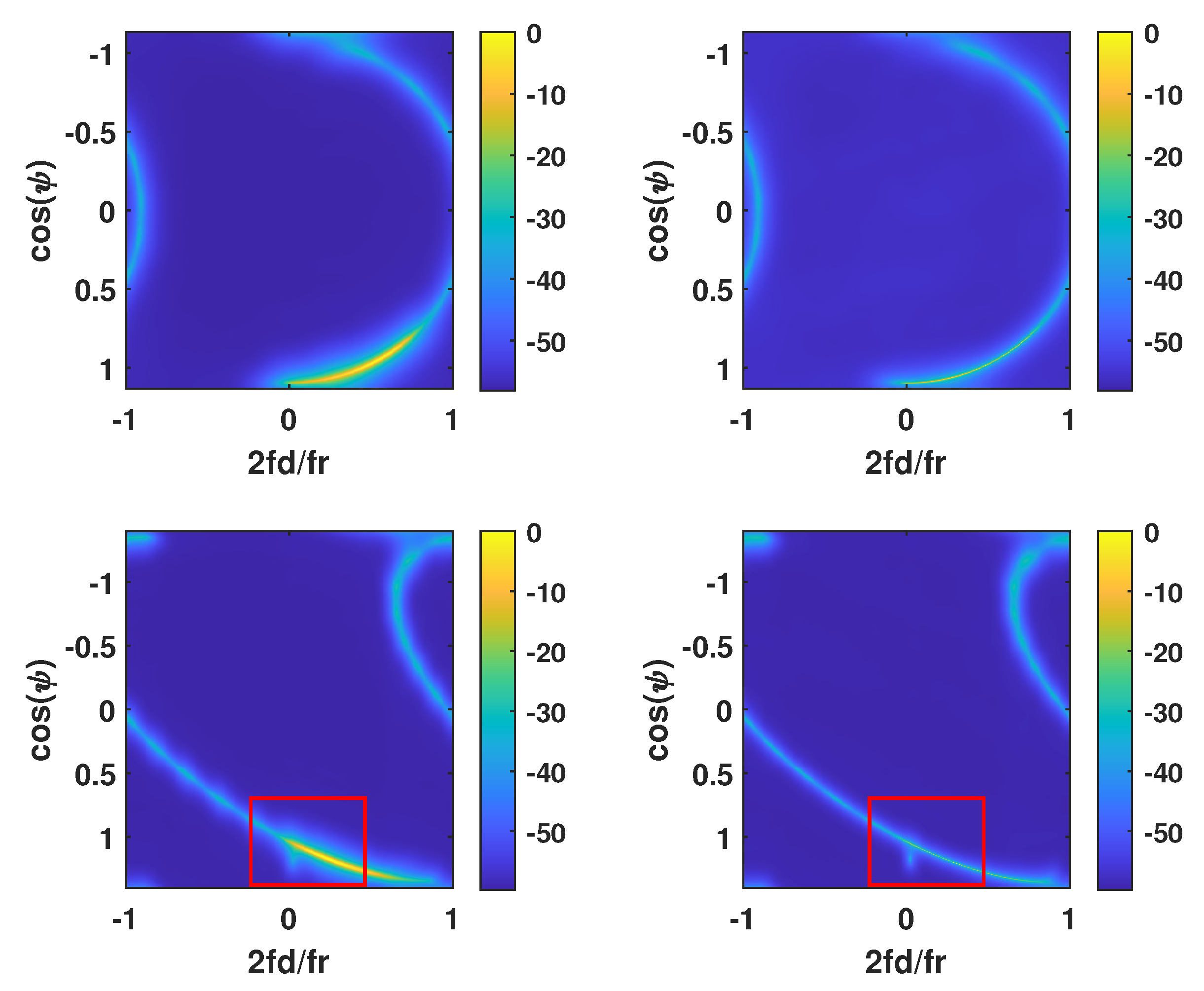
4.1. Space–Time Distribution of the Clutter Spectrum

Figure 1 depicts the clutter spectrum of the proposed algorithm in spatial and temporal domains, where the left sub-figures correspond to the original STAP processor and the right ones correspond to the proposed processor. The non-side-looking angle is ϑ = 50 . Moreover, N = 14 , K = 20 , L = 250 , v a = 105 m/s, v c = 95 m/s, CNR = 45 dB, and the two bottom sub-figures contain the target. Figure 1 shows that due to the differences of the clutter spectrum distributions of the L range cells, the method of direct sample averaging of adjacent range cells leads to the serious broadening of clutter spectrum, which further leads to the serious degradation of the STAP processor, especially the performance of the mainlobe clutter suppression. This simulation verifies that through the proposed method, the clutter spectrum is obviously narrowed, which is beneficial for highlighting the target as can be seen in the red box of the bottom-right sub-figure. The similarity degree of clutter from different range cells is increased, indicating the effectiveness of the proposed method.

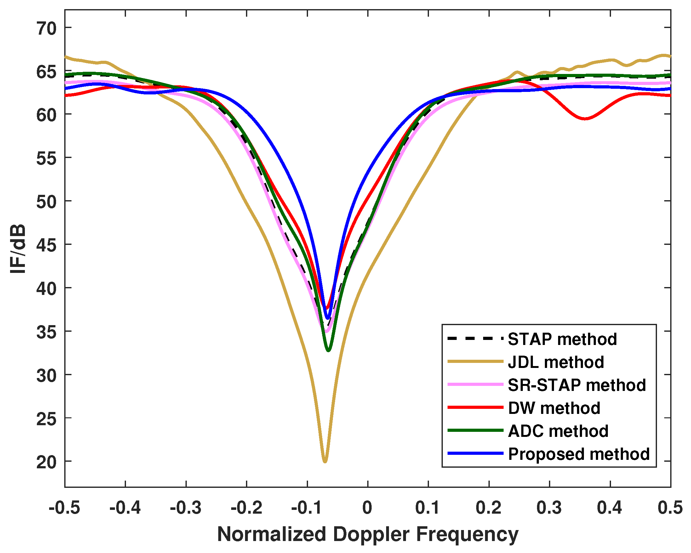
4.2. Results of the Improvement Factor

The relationship between the IF and normalized Doppler frequency is demonstrated in Figure 2. The clutter suppression results of different methods for different conditions are evaluated. Specifically, ϑ = −90°, N = 13 , K = 16 , L = 70 , v a = 70 m/s, v c = 130 m/s, and CNR = 80 dB in Figure 2. The results show that the severe broadening of the IF curve notches occurs for the STAP and JDL methods, and after range compensation using the DW and ADC methods, the non-uniformity of the clutter is improved. Overall, the IF notch of the proposed algorithm is kept the narrowest compared to the others, indicating that the proposed algorithm can achieve better clutter suppression performance than the other methods.
The results of IF with different radar and clutter conditions are presented in Figure 3. The differences are ϑ = 75 , v a = 55 m/s, v c = 120 m/s, and CNR = 70 dB. They show that compared with the others, the proposed algorithm still possesses clear advantages with a narrower IF curve notch. It indicates that the proposed algorithm reduces the possibility of the target submersion in the broadened clutter spectrum, and it enhances the performance of detection by increasing the output ratio of the signal-to-clutter power. Moreover, the ADC method is better than the methods of STAP, DW, JDL, and SR-STAP based on sparse M-FOCUSS because of its effective range compensation that improves the uniformity of clutter.
For a further comprehensive evaluation, different methods under conditions v a = 85 m/s, v c = 118 m/s, CNR = 65 dB, and L = 100 are considered as shown in Figure 4, whose other conditions are consistent with Figure 3. The proposed method maintains an outstanding ability of clutter suppression, as can be seen from its high IF curve with a narrow and deep IF notch. This indicates that with a desired performance, the proposed method can be applicable to different radar and signal environments adaptively.

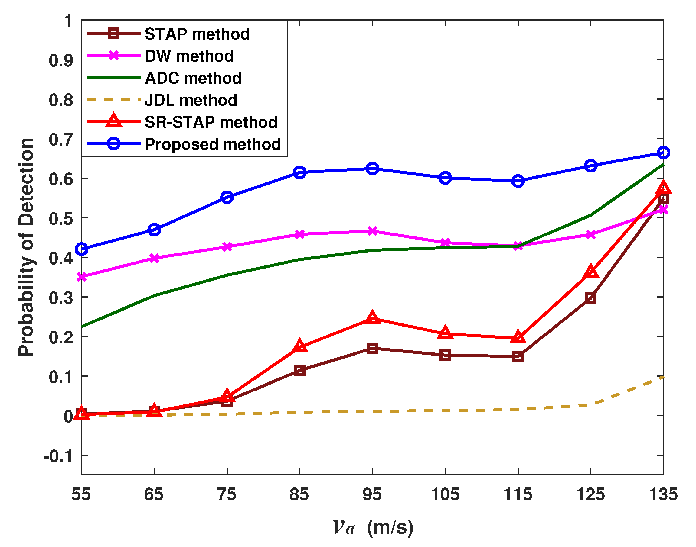
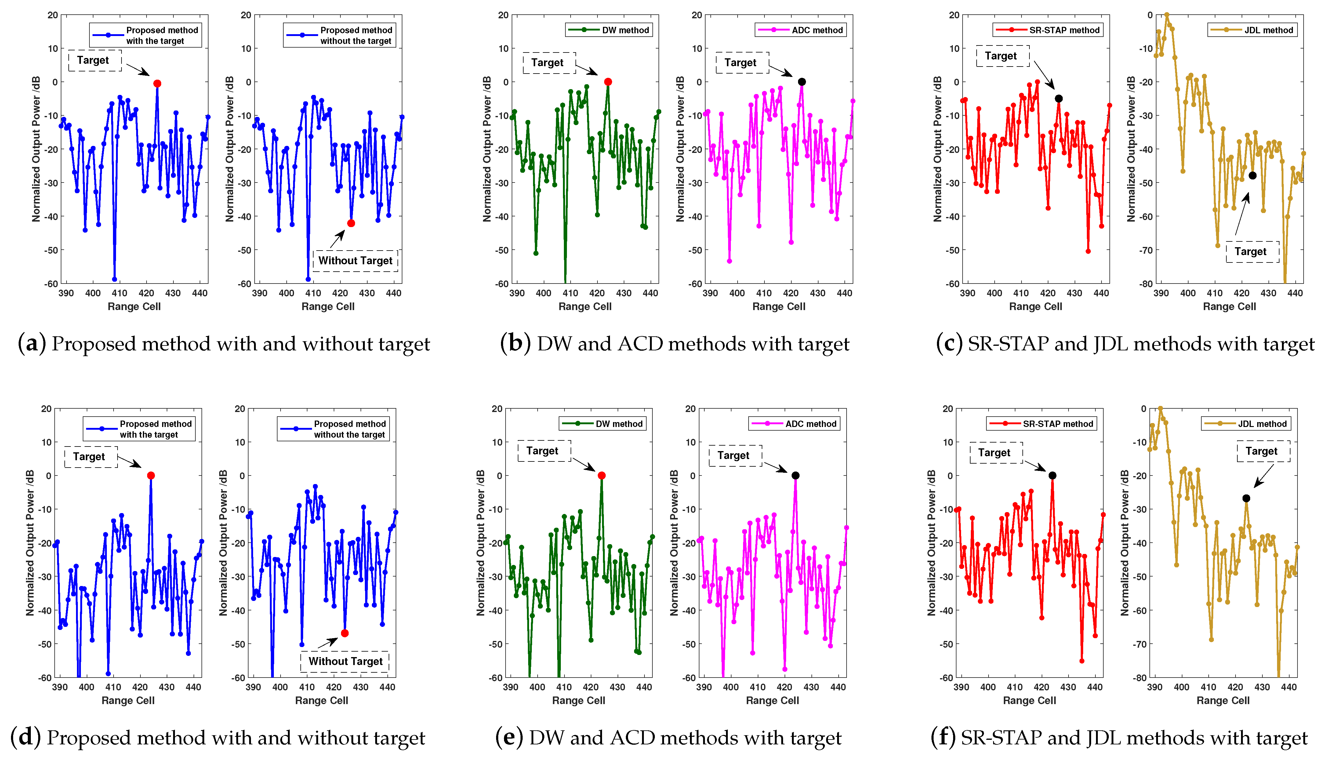
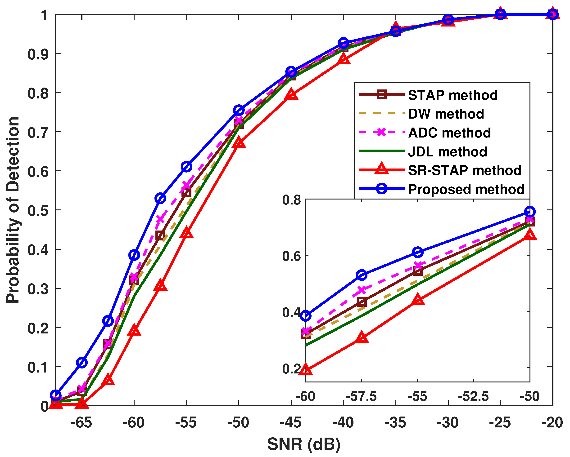
4.3. Results of the Probability of Detection

By comparing the probability of detection, abbreviated as PD under variational SNR circumstances, different methods are evaluated in Figure 5 to demonstrate the performance of target detection. Another radar configuration and target environment is considered for a more comprehensive assessment of the proposed method, that is, N = 11 , K = 18 , v a = 120 m/s, v c = 90 m/s, ϑ = 90 , CNR = 70 dB, and L = 70 . When detecting the target, the commonly applied constant false alarm rate (CFAR) [38] with cell averaging is brought in, and its false alarm probability is PFA = 10 5 for all the methods. It can be concluded that within the entire scope of the considered SNR, the proposed algorithm accomplishes the highest PD among different methods, indicating that it owns the best performance in this condition.
Figure 6 shows the PD versus SNR for different methods under N = 6 , K = 18 , v a = 130 m/s, v c = 105 m/s, ϑ = 75 , CNR = 65 dB, and L = 70 . Among the analyzed methods in Figure 6, the target detection of the proposed method is the best with the maximal probability of successfully detecting the target. The advantages of the proposed method remain significant within a large range of SNR.

4.4. Influence of Different Radar Circumstances

Figure 7 shows the impact of the numbers ( N , K ) of array elements and coherent pulses in radar configuration on the performance of different methods. The changed N and K are considered; meanwhile, the other circumstances are consistent with those in Figure 5, except that SNR = 5 dB and CNR = 65 dB. Figure 7 demonstrates that, usually, the decrease in N and K leads to decreased probabilities of target detection for all the methods. In addition, the three algorithms that carried out range compensation show significantly higher probabilities than the others, and the proposed method is superior throughout the variations in the considered N and K.
Figure 8 shows the PD versus the radar platform speed to evaluate the influence of v a on different methods, where the differences from Figure 3 are N = 10 , K = 18 , and ϑ = 90 , and v a changes from v a = 55 m/s to v a = 135 m/s. From Figure 8, with the increasing v a , the rising trend of the detection probability can be observed for the methods. Furthermore, the proposed method is always advantageous for different radar circumstances including the varying v a .

4.5. Test Errors of the Proposed Network

Figure 9 shows the test errors of the proposed network versus the number of samples, where root mean square error (RMSE) and standard deviation (STD) with different numbers Ns of array elements are evaluated. Its conditions are consistent with those of Figure 6. Figure 9 indicates that with the increased samples, the evaluation of the proposed network gets better and gradually tends to be stable. The proposed network is convergent; moreover, it achieves a good performance in clutter suppression, range compensation, and further target detection, as can be seen from Figure 1, Figure 2, Figure 3, Figure 4, Figure 5, Figure 6, Figure 7, Figure 8 and Figure 9.

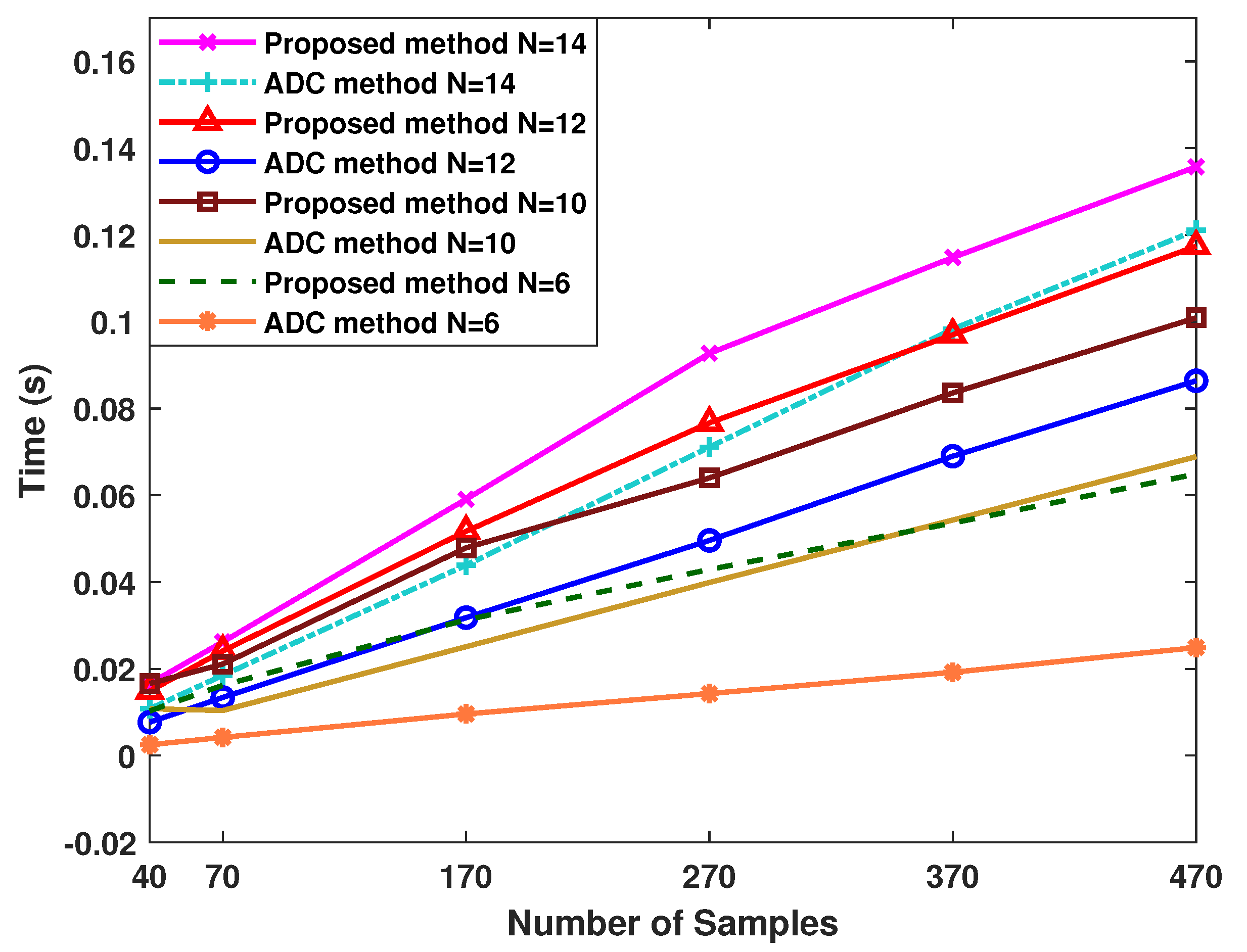
4.6. Comparison of the Computation Time

In Figure 10, computation time is shown under the changing numbers of training samples and array elements, where v a = 130 m/s, v c = 105 m/s, ϑ = 90 , and CNR = 65 dB. Additionally, the sample number changes from L = 40 to L = 470 , and in the meantime, N is considered as N = 6 , N = 10 , N = 12 , and N = 14 . The typical range compensation ADC method is served as a contrast. From Figure 10, the influence of the numbers of samples and array elements on the computation time manifests the following trend: the smaller L contributes to the closer computation time between the proposed method and the ADC method. Additionally, the difference in their computation time becomes small with the increased N, and the time of the proposed method is reasonable. Although the proposed method costs more time, it provides significant advantages over the ADC method as demonstrated in Figure 2, Figure 3, Figure 4, Figure 5, Figure 6, Figure 7 and Figure 8.

4.7. Results with Experimental Data

Experimental data are used to validate the performance advantages of the proposed method. Different methods are applied to the real data, which are multi-channel airborne radar measurements (MCARM) [39]. The real clutter environment of airborne radar is reflected by the data containing various types of clutter such as ground, sea, ground-sea transition, and urban areas. Errors related to array antennas unavoidably occur when collecting data with airborne radar. Importantly, there is a yaw angle ϑ = 7 . 28 . As a result, the experimental data can effectively validate the clutter suppression performance of different methods under the conditions of non-IID samples in non-side-looking airborne radar.
Figure 11 shows the comparison of IF in clutter suppression performance for processing experimental data. The data are obtained from the range cells l = 250 to l = 350 , and they are located in a region with strong clutter. The specific parameters of the radar platform can be found in [39]. Figure 11 indicates that all methods exhibit a decrease in performance after applying the real experimental data. This is caused by the more serious non-uniform clutter from the factors such as array element errors and parameter estimation biases in the real environment. However, compared to the other methods, the proposed method still exhibits a narrower IF notch, reducing the possibility of target submersion in the broadened clutter spectrum. Therefore, the proposed method is effective and advantageous when applied to experimental data.
In order to visually verify the performance of the proposed method applied to experimental data, Figure 12 displays a comparison of the normalized output power of different clutter suppression methods. The range cells corresponding to the clutter to be processed are from l = 388 to l = 438 . A target is injected into the l = 425 th range cell to visually validate the clutter suppression results. The normalized Doppler frequency of the target is 0.05 , located in the main clutter region. In addition, the output power of the range cell with the target is labeled. When comparing, all methods’ processes are applied on the same clutter data.
In Figure 12a–c, it can be observed that only the proposed algorithm whose output signal power is the most prominent, effectively detects the target, while the targets in the other methods are almost submerged in clutter when SCR = −55 dB. Additionally, in the same clutter environment, the left and the right sub-figures in Figure 12a correspond to the scenarios with and without the target, respectively. This indicates that the proposed algorithm does not cause the false alarm. Therefore, the proposed method can provide a superior clutter suppression performance with the experimental data.
In Figure 12d–f, the output power of all the methods is improved in terms of the target range cell with the increased SCR = −50 dB. Under the circumstances, the proposed algorithm distinguishes the target from the clutter clearly, indicating its good performance in target detection.
Figure 13 demonstrates the target detection probabilities of different methods for the experimental data, with the parameters of the real clutter data being the same as Figure 12. In the actual clutter environment, a random target is injected into the range cell l = 425 and detected by different methods. By injecting the target randomly 300 times, the probability of successfully detecting the target is evaluated. Additionally, PFA = 10 5 is the same for all the methods. Figure 13 shows that the proposed method provides a higher detection probability within a large SCR range, further verifying that it can be applied to real clutter environments. The proposed algorithm achieves an effective range compensation and better clutter suppression, thereby improving the performance of target detection.

5. Discussion

Discussion 1: The reasonable computation time of the proposed algorithm is primarily due to the utilization of ELM theory when training the network for range compensation and clutter suppression. That is, the weight matrix W 0 and bias vector b 0 are set randomly, and the output weight matrix Υ 0 can be directly obtained. Therefore, the computational complexity of network training is significantly reduced, requiring only O [ min ( H 2 L , L 2 H ) ] . Then, the proposed compensation matrix estimation and reconstruction further require an O [ H 2 L + 32 ( H 2 L + H 2 ) ] computation, mainly caused by the matrix multiplications from Equations (26) and (34)–(42). Accordingly, considering the process of matrix inversion involved in the designed objective output O [ ( N K ) 3 ] , the computation burden of the proposed algorithm is about O [ ( N K ) 3 + min ( H 2 L , L 2 H ) + 33 H 2 L + 32 H 2 ] . With a reasonable computation time, the proposed algorithm greatly improves the performance of radar target detection.
Discussion 2: The following main reasons and novelties contribute to the performance advantages of the proposed algorithm. Firstly, a reverse feedback iterative process driven by the specifically designed objective outputs is proposed to estimate the compensation matrix. A reweighted network with an unknown compensation matrix involved in training and updating is designed. Secondly, the proposed algorithm maximally preserves the information of complex values. The theoretical derivation processes of the compensation matrix estimation and reconstruction in complex form are proposed in detail. Thirdly, the proposed algorithm requires fewer additional parameter settings. Only the update step size ξ and the scaling factor ε need to be set during training and reconstruction, and they have little impact on the algorithm performance. Fourthly, the proposed algorithm is adaptive, continuously updating the compensation matrix estimation to match the current objective data condition.
Discussion 3: The main drawback of the proposed algorithm is that the calculation time is slightly higher than that of the range compensation ADC method. Additionally, when constructing the loss function and setting the initial range compensation matrix for network training, it is still hoped to exploit some radar system parameters to further improve the convergence and the iteration time. However, unlike most of the range compensation methods, the proposed algorithm does not heavily rely on the system inertial parameters, on account of the proposed adaptive and continuous updating of the compensation matrix under the designs of the specific objective outputs and the data-driven conditions.
Discussion 4: The proposed algorithm mainly aims at the clutter amplitude model of the Rayleigh distribution, which is generally used to describe meteorological clutter, chaff interference, as well as ground clutter and sea clutter of low- and medium-resolution radar systems with large incident angles. Apart from this distribution, there are other clutter models such as K distribution, Weibull distribution, and Log-normal distribution. The non-uniformity of clutter samples in these non-Gaussian models may be more serious, which leads to a relative large decrease in the performance of the proposed method and the traditional methods involving the CNCM estimation.
Specifically, the impact of other clutter models on the proposed method is that during the process of the proposed initial network training, the design of the objective outputs o 1 ( l ) and o 3 ( l ) mainly focuses on range compensation. It refers to the non-uniform situation caused by the non-side-looking array and does not aim at other non-uniform factors. In addition, the design of the objective outputs o 2 ( l ) and o 4 ( l ) involves CNCM. However, the estimation accuracy of this covariance matrix is degraded due to non-Gaussian models such as K distribution. Therefore, they affect the training of the initial network of the proposed algorithm, resulting in bias in the designed subsequent estimation of the unknown range compensation matrix. Through pre-processing that improves the CNCM estimation and through further designing specialized initial network training, future related research that specifically aims at other clutter models and other non-uniform factors can be developed based on the proposed method.

6. Conclusions

In this paper, we propose a reweighted extreme learning machine-based clutter-suppression and range-compensation method for non-side-looking airborne radar. In the proposed algorithm, after designing the pre-processing, the special reweighted complex-valued activation function, and two new objective outputs, the initial training of the reweighted ELM-based network is constructed. Then, by proposing two other objective outputs, the new loss function, the objective data-driven reverse-feedback framework, and the special processes of the complex structures and the theoretical derivations for estimating the unknown compensation matrix, the samples are updated and compensated for clutter suppression and target detection. The reasons for the reasonable computational complexity and for the advantages of the proposed algorithm are analyzed, and the simulation results verify that the proposed algorithm provides superior clutter suppression with effective range compensation. Moreover, the proposed algorithm achieves obviously higher detection probabilities and better improvement factors.

Author Contributions

Conceptualization, J.L. and G.L.; methodology, J.L.; software, J.L.; formal analysis, J.L. and C.Z.; resources, J.L., C.Z. and H.T.; writing—original draft preparation, J.L.; writing—review and editing, J.L. and F.H.J.; project administration, J.L., S.Z. and J.X.; funding acquisition, J.L., C.Z., G.L. and H.T.; supervision, J.L., J.X., S.Z. and F.H.J. All authors have read and agreed to the published version of the manuscript.

Funding

This work was supported by the National Natural Science Foundation of China (NSFC) under Grant 61931016, 62071344, and 61901340, and the stabilization support of the National Radar Signal Processing Laboratory under Grant KGJ20230X.

Data Availability Statement

Not applicable due to privacy.

Conflicts of Interest

The authors declare no conflicts of interest.

References

  1. Klemm, R. Principles of Space-Time Adaptive Processing; The Institution of Electrical Engineers: London, UK, 2002. [Google Scholar]
  2. Lapierre, F.; Droogenbroeck, M.V.; Verly, J.G. New methods for handling the dependence of the clutter spectrum in non-sidelooking monostatic STAP radars. In Proceedings of the 2003 IEEE International Conference on Acoustics, Speech, and Signal Processing, Hong Kong, China, 6–10 April 2003; pp. 73–76. [Google Scholar]
  3. Lapierre, F.D.; Ries, P.; Verly, J.G. Foundation for mitigating range dependence in radar space-time adaptive processing. IET Radar Sonar Navig. 2009, 3, 18–29. [Google Scholar] [CrossRef]
  4. Lapierre, F.; Verly, J.G. Computationally-efficient range dependence compensation method for bistatic radar STAP. In Proceedings of the IEEE International Radar Conference, Arlington, VA, USA, 9–12 May 2005; pp. 714–719. [Google Scholar]
  5. Kreyenkamp, O.; Klemm, R. Doppler compensation in forward-looking STAP radar. IEE Proc. Radar Sonar Navig. 2001, 148, 253–258. [Google Scholar] [CrossRef]
  6. Borsari, G.K. Mitigating effects on STAP processing caused by an inclined array. In Proceedings of the 1998 IEEE Radar Conference, Dallas, TX, USA, 14 May 1998; pp. 135–140. [Google Scholar]
  7. Himed, B.; Zhang, Y.; Hajjari, A. STAP with angle-Doppler compensation for bistatic airborne radars. In Proceedings of the IEEE Radar Conference, Long Beach, CA, USA, 25 April 2002; pp. 311–317. [Google Scholar]
  8. Lapierre, F.D.; Verly, J.G. Registration-based range-dependence compensation for bistatic STAP radars. EURASIP J. Appl. Signal Process. 2005, 1, 85–98. [Google Scholar] [CrossRef]
  9. Wang, Y.; Peng, Y. Space-time joint processing method for simultaneous clutter and jamming rejection in airborne radar. Electron. Lett. 1996, 32, 258. [Google Scholar] [CrossRef]
  10. Dipietro, R.C. Extended factored space-time processing for airborne radar systems. In Proceedings of the 26th Asilomar Conference, Pacific Grove, CA, USA, 26–28 October 1992; pp. 425–430. [Google Scholar]
  11. Wang, Y.L.; Chen, J.W.; Bao, Z.; Peng, Y.N. Robust space-time adaptive processing for airborne radar in nonhomogeneous clutter environments. IEEE Trans. Aerosp. Electron. Syst. 2003, 39, 70–81. [Google Scholar] [CrossRef]
  12. Brown, R.D.; Schneible, R.A.; Wicks, M.C.; Wang, H.; Zhang, Y.H. STAP for clutter suppression with sum and difference beams. IEEE Trans. Aerosp. Electron. Syst. 2000, 36, 634–646. [Google Scholar] [CrossRef]
  13. Goldstein, J.S. Reduced rank adaptive filtering. IEEE Trans. Signal Process. 1997, 45, 492–496. [Google Scholar] [CrossRef]
  14. Goldstein, J.S.; Reed, I.S.; Scharf, L.L. A multistage representation of the Wiener filter based on orthogonal projections. IEEE Trans. Inf. Theor. 1998, 44, 2943–2959. [Google Scholar] [CrossRef]
  15. Zhang, M.; Zhang, A.X.; Li, J.X. Fast and accurate rank selection methods for multistage Wiener filter. IEEE Trans. Signal Process. 2016, 64, 973–984. [Google Scholar] [CrossRef]
  16. Cotter, S.F.; Rao, B.D.; Engan, K.; Delgado, K.K. Sparse solutions to linear inverseproblems with multiple measurement vectors. IEEE Trans. Signal Process. 2005, 53, 2477–2488. [Google Scholar]
  17. Bai, G.; Tao, R.; Zhao, J.; Bai, X. Parameter-searched OMP method for eliminating basis mismatch in space-time spectrum estimation. Signal Process. 2017, 138, 11–15. [Google Scholar] [CrossRef]
  18. Ji, S.; Xue, Y.; Carin, L. Bayesian compressive sensing. IEEE Trans. Signal Process. 2008, 56, 2346–2356. [Google Scholar] [CrossRef]
  19. Li, Z.H.; Zhang, Y.S.; He, X.Y.; Guo, Y.D. Low-complexity off-grid STAP algorithm based on local search clutter subspace estimation. IEEE Geosci. Remote Sens. Lett. 2018, 15, 1862–1866. [Google Scholar] [CrossRef]
  20. Han, S.D.; Fan, C.Y.; Huang, X.T. A novel STAP based on spectrum-aided reduced-dimension clutter sparse recovery. IEEE Geosci. Remote Sens. Lett. 2017, 14, 213–217. [Google Scholar] [CrossRef]
  21. Liu, J.; Zhou, W.D.; Juwono, F.H.; Huang, D.F. Reweighted smoothed l0-norm based DOA estimation for MIMO radar. Signal Process. 2017, 137, 44–51. [Google Scholar] [CrossRef]
  22. Yang, Z.; Lamare, R.C.D.; Li, X.; Wang, H. Knowledge-aided stap using low rank and geometry properties. Int. J. Antennas Propag. 2014, 2014, 196507. [Google Scholar] [CrossRef]
  23. Chen, W.C.; Chen, B.; Liu, Y.C.; Wang, C.J.; Peng, X.J.; Liu, H.W.; Zhou, M.Y. Infinite switching dynamic probabilistic network with Bayesian nonparametric learning. IEEE Trans. Signal Process. 2022, 70, 2224–2238. [Google Scholar] [CrossRef]
  24. Duan, K.; Chen, H.; Xie, W.; Wang, Y. Deep learning for high-resolution estimation of clutter angle-Doppler spectrum in STAP. IET Radar Sonar Navig. 2022, 16, 193–207. [Google Scholar] [CrossRef]
  25. Li, H.; Zhuang, L.; Guan, Y.; Wang, J. A machine learning approach for clutter suppression in airborne radar based on multitask learning. IEEE Access 2020, 8, 22541–22552. [Google Scholar]
  26. Huang, G.B.; Zhu, Q.Y.; Siew, C.K. Extreme learning machine: Theory and applications. Neurocomputing 2006, 70, 489–501. [Google Scholar] [CrossRef]
  27. Huang, G.; Song, S.; Gupta, J.N.; Wu, C. Semi-supervised and unsupervised extreme learning machines. IEEE Trans. Cybern. 2014, 44, 2405–2417. [Google Scholar] [CrossRef]
  28. Huang, G.B.; Zhu, Q.Y.; Siew, C.K. Extreme learning machine: A new learning scheme of feedforward neural networks. In Proceedings of the IEEE International Joint Conference on Neural Network, Budapest, Hungary, 25–29 July 2004; Volume 2, pp. 985–990. [Google Scholar]
  29. Zou, B.; Wang, X.; Feng, W.; Zhu, H.; Lu, F. DU-CG-STAP method based on sparse recovery and unsupervised learning for airborne radar clutter suppression. Remote Sens. 2022, 14, 3472. [Google Scholar] [CrossRef]
  30. Mou, X.; Chen, X.; Guan, J.; Dong, Y.; Liu, N. Sea clutter suppression for radar PPI images based on SCS-GAN. IEEE Geosci. Remote Sens. Lett. 2020, 18, 1886–1890. [Google Scholar] [CrossRef]
  31. Li, G.Q.; Song, Z.Y.; Guan, J.; Fu, Q. A convolutional neural network based approach to sea clutter suppression for small boat detection. Front. Informa. Technol. Electron. Eng. 2020, 21, 1504–1520. [Google Scholar] [CrossRef]
  32. Liu, J.; Liao, G.S.; Xu, J.W.; Zhu, S.Q.; Juwono, F.J.; Zeng, C. Autoencoder neural network-based STAP algorithm for airborne radar with inadequate training samples. Remote Sens. 2022, 14, 6021. [Google Scholar] [CrossRef]
  33. Liu, J.; Liao, G.S.; Xu, J.W.; Zhu, S.Q.; Zeng, C.; Juwono, F.J. Unsupervised affinity propagation clustering based clutter suppression and target detection algorithm for non-side-looking airborne radar. Remote Sens. 2023, 15, 2077. [Google Scholar] [CrossRef]
  34. Zaimbashi, A. An adaptive cell averaging-based CFAR detector for interfering targets and clutter-edge situations. Digit. Signal Process. 2014, 31, 59–68. [Google Scholar] [CrossRef]
  35. Liu, W.J.; Liu, J.; Hao, C.P.; Gao, Y.C.; Wang, Y.L. Multichannel adaptive signal detection: Basic theory and literature review. Sci. China Inf. Sci. 2022, 65, 121301. [Google Scholar] [CrossRef]
  36. Xu, J.W.; Liao, G.S.; Huang, L.; Zhu, S.Q. Joint magnitude and phase constrained STAP approach. Digit. Signal Process. 2015, 46, 32–40. [Google Scholar] [CrossRef]
  37. Ottersten, B.; Stoica, P.; Roy, R. Covariance matching estimation techniques for array signal processing applications. Digit. Signal Process. 1998, 8, 185–210. [Google Scholar] [CrossRef]
  38. Gini, F.; Greco, M. Covariance matrix estimation for CFAR detection in correlated heavy tailed clutter. Signal Process. 2002, 82, 1847–1859. [Google Scholar] [CrossRef]
  39. Sarkar, T.K.; Wang, H.; Park, S.; Adve, R.; Koh, J.; Kim, K.; Zhang, Y.; Wicks, M.C.; Brown, R.D. A deterministic least-squares approach to space-time adaptive processing. IEEE Trans. Antennas Propag. 2001, 49, 91–103. [Google Scholar] [CrossRef]
Figure 1. Space–time clutter spectra for the original STAP method (left) and the proposed method (right).
Remotesensing 16 01093 g001
Figure 2. Comparison of IF with the variation of normalized Doppler frequency.
Remotesensing 16 01093 g002
Figure 3. IF versus normalized Doppler frequency under different conditions.
Remotesensing 16 01093 g003
Figure 4. IF versus normalized Doppler frequency for different radar and signal circumstances.
Remotesensing 16 01093 g004
Figure 5. Comparison of PD with the variation of SNR.
Remotesensing 16 01093 g005
Figure 6. Comparison of PD with the variation of SNR under different conditions.
Remotesensing 16 01093 g006
Figure 7. Influence of array elements and pulses on detection probabilities of different methods.
Remotesensing 16 01093 g007
Figure 8. Influence of platform speed on detection probabilities of different methods.
Remotesensing 16 01093 g008
Figure 9. RMSE and STD versus the number of samples for the proposed network.
Remotesensing 16 01093 g009
Figure 10. Relationship between computation time and number of samples.
Remotesensing 16 01093 g010
Figure 11. IF comparison of different methods with experimental data.
Remotesensing 16 01093 g011
Figure 12. Normalized output power for different range cells. (ac) Different methods with SCR = −55 dB. (df) Different methods with SCR = −50 dB.
Remotesensing 16 01093 g012
Figure 13. Target detection performance of different methods with data of actual clutter environment.
Remotesensing 16 01093 g013
Disclaimer/Publisher’s Note: The statements, opinions and data contained in all publications are solely those of the individual author(s) and contributor(s) and not of MDPI and/or the editor(s). MDPI and/or the editor(s) disclaim responsibility for any injury to people or property resulting from any ideas, methods, instructions or products referred to in the content.

