Optimal Configuration of Omega-Kappa FF-SAR Processing for Specular and Non-Specular Targets in Altimetric Data: The Sentinel-6 Michael Freilich Study Case

Abstract

In this study, the full-focusing (FF) algorithm is reviewed with the objective of optimizing it for processing data from different types of surfaces probed in altimetry. In particular, this work aims to provide a set of optimal FF processing parameters for the Sentinel-6 Michael Freilich (S6-MF) mission. The S6-MF satellite carries an advanced radar altimeter offering a wide range of potential FF-based applications which are just beginning to be explored and require prior optimization of this processing. In S6-MF, the Synthetic Aperture Radar (SAR) altimeter acquisitions are known to be aliased in the along-track direction. Depending on the target, aliasing can be tolerated or may be a severe impairment to provide the level of performance expected from FF processing. Another key aspect to consider in this optimization study is the unprecedented resolution of the FF processing, which results in a higher posting rate than the standard SAR processing. This work investigates the relationship between posting rate and noise levels and provides recommendations for optimal algorithm configurations in various scenarios, including transponder, open ocean, and specular targets like sea-ice and inland water scenes. The Omega–Kappa (WK) algorithm, which has demonstrated superior CPU efficiency compared to the back-projection (BP) algorithm, is considered for this study. But, unlike BP, it operates in the Doppler frequency domain, necessitating further precise spectral and time domain settings. Based on the results of this work, real case studies using S6-MF acquisitions are presented. We first compare S6-MF FF radargrams with Sentinel-1 (S1) images to showcase the potential of optimally configured FF processing. For highly specular surfaces such as sea-ice, distinct techniques are employed for lead signature identification. S1 relies on image-based lineic reconstruction, while S6-MF utilizes phase coherency of focalized pulses for lead detection. The study also delves into two-dimensional wave spectra derived from the amplitude modulation of image/radargrams, with a focus on a coastal example. This case is especially intriguing, as it vividly illustrates different sea states characterized by varying spectral peak positions over time.

1. Introduction

The full-focusing (FF) algorithm, initially introduced in altimetry by [1], coherently processes a synthetic aperture of pulse echoes produced by pulse-limited nadir-looking radar altimeters within the whole target illumination time. This technique closely resembles the one used in synthetic aperture radar (SAR) imagery, offering the potential to enhance along-track resolution up to its theoretical limit, which is half the antenna length. The FF approach enables mapping of the overflown surface with unprecedented precision, revealing features like open-water leads [2,3], inland waters [4], coastal regions [5] and small-scale ocean structures [6]). Additionally, it holds the promise of providing a more detailed estimation of the geophysical parameters compared to unfocused (UF) SAR processing. It is to be noted that the high FF performance is only attained if the pulse-to-pulse stability (in phase and amplitude) is ensured within the entire synthetic aperture length, which necessitates a time period considerably longer than the burst duration. In cases where water surfaces decorrelate quickly over time, the FF resolution may degrade [7], with a more pronounced impact over open ocean compared to lakes.

Recognizing the advantages of FF over standard unfocused processing [1], we decided to apply it to process Sentinel-6 Michael Freilich (S6-MF) data. However, the original back-projection (BP) algorithm, while highly accurate, proves computationally demanding for operational processors. To address this challenge, a frequency-based method [8] known as the Omega–Kappa (WK) processor was introduced. This algorithm is analogous to the one used for traditional SAR data, but it incorporates a different focusing operator due to the high carrier frequency used by altimeters, specifically Ku and, soon, Ka bands [9]). This frequency choice prohibits neglecting the Doppler frequency shift resulting from the relative motion between the altimeter and the target in impulse response modeling. The WK algorithm offers a substantial processing speed advantage, which is up to two orders of magnitude faster compared to BP, making it eligible for future operational FF processors.

It is worth noting that WK operator re-formulation is essential for onboard deramped altimeters such as Cryosat-2 (C2). The radar altimeters create onboard pre-processing to select only a few samples located where the nadir scattering energy is expected. This avoids the transfer of a large amount of useless data on the ground and facilitates waveform-leading edge detection. While C2 [10] employs deramping, S6-MF uses a matched filtering approach [11].

Moreover, S6-MF distinguishes itself as the first SAR altimeter with nearly continuous pulse sampling, whereas Sentinel-3 (S3) and C2 operate in a non-continuous burst emission mode of pulses, resulting in a set of replicas or ghosts for each target response. Closed-burst acquisitions generate replicas, which can distort the surface signal through complex interference phenomena. This issue poses a significant limitation to FF processing in closed-burst acquisition mode, especially when it comes to estimating water surface height over specular targets, which may be less reliable than the unfocused (UF) processing. Open-burst mode data are found to be optimal for FF processing, as evidenced by S6-MF. Notably, S6-MF includes two missing pulses generating replicas every 300 m, with substantially weaker amplitudes compared to closed-burst missions [11]. These weaker replicas offer an opportunity to explore techniques for further mitigation.

The breakthrough resolution provided by FF, with its superior signal-to-noise ratio compared to UF, allows for unprecedented observations of highly specular surfaces such as inland water and sea-ice leads. These observations take the form of radargrams resembling SAR folded images, providing a two-dimensional representation of a scene with half-meter resolution. This capability enables SAR altimetry to be leveraged like SAR imagery, enabling applications like two-dimensional wave spectra, water shapefile projection, and more. In hydrology, these images facilitate measurements of water level, extent, and geolocation of off-nadir rivers and lakes [4]. In open-ocean settings, FF radargrams can reveal swell waves’ signatures as amplitude modulations, permitting the derivation of two-dimensional spectra characterizing swell features [6].

This paper aims at providing a set of optimal processing parameters for FF processing across different ground target scenarios. The WK processor shall be taken as a reference, although the considerations in Section 2 are valid for the BP processor as well. Additionally, the paper explores aspects that have received limited attention in the literature, including replica mitigation, mean square slope (MSS) and its relationship with Doppler bandwidth, and the trade-off between resolution and noise level. The fine-tuning of the FF processor to specific target characteristics is crucial for unlocking FF’s full potential in imaging the surfaces observed by S6-MF. Specifically, the paper investigates five parameters or processing options:

• Percentage of Doppler bandwidth: S6-MF experiences aliasing in the along-track direction due to the wide antenna mainlobe relative to the pulse repetition frequency (PRF). Decisions regarding where to truncate have a substantial impact on the final resolution.
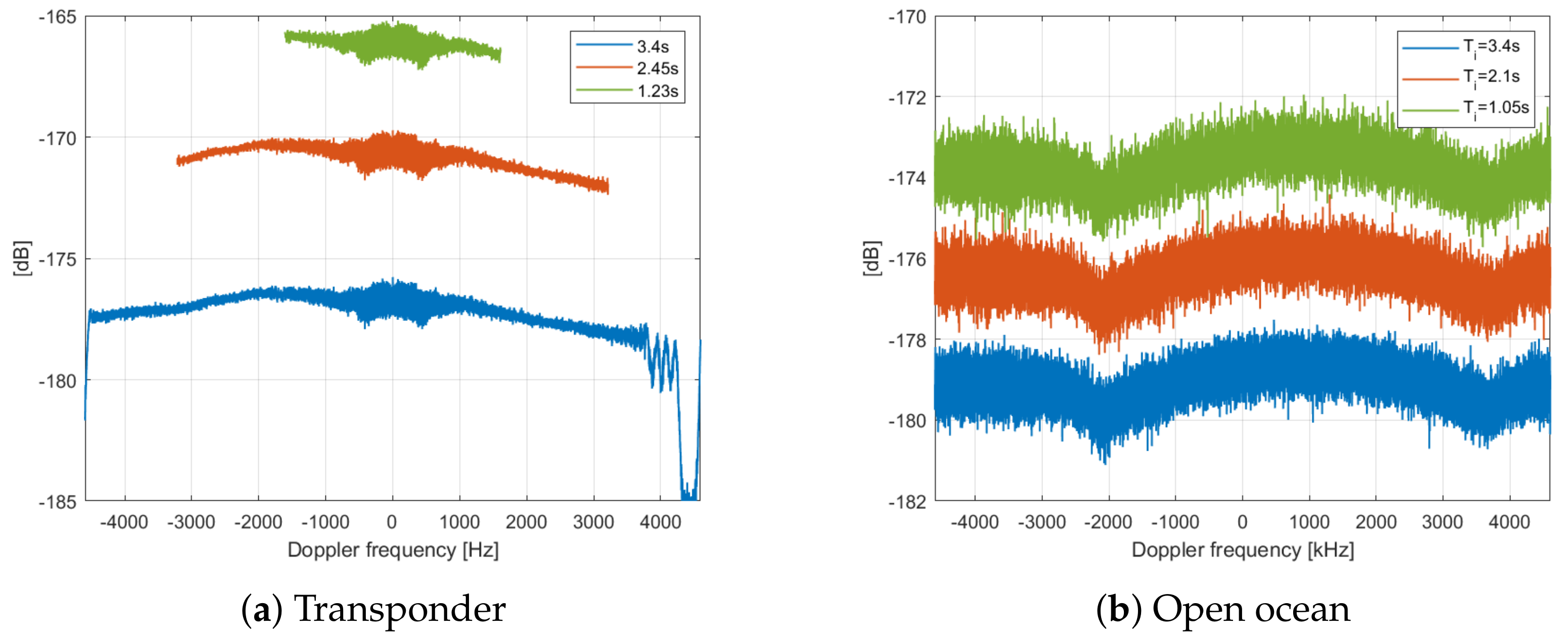
• Integration time: This parameter is closely linked to resolution and assumes critical importance, particularly for highly specular targets (i.e., low MSS), as discussed in detail below.
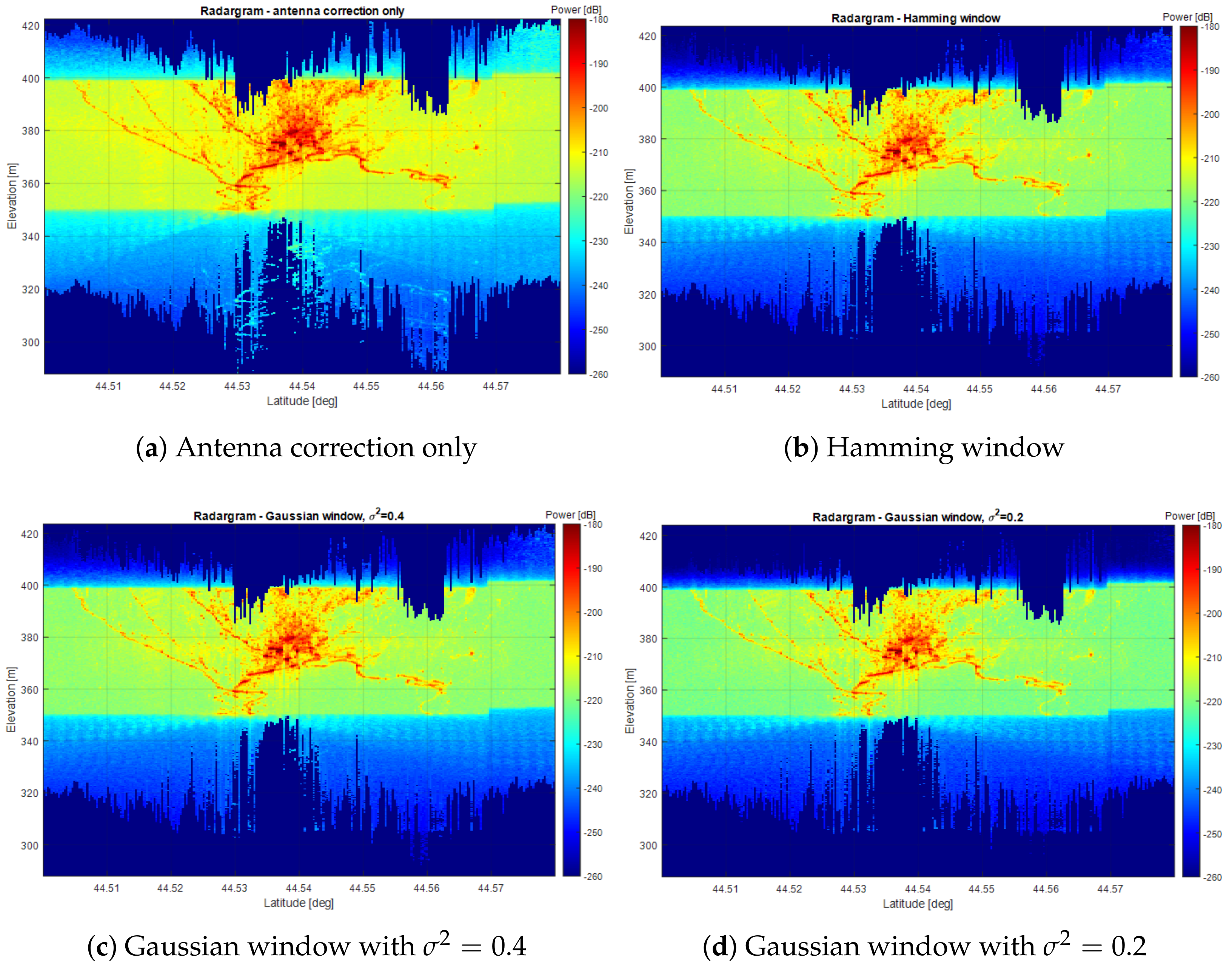
• Doppler windows: This aspect involves antenna compensation (whether to apply it or not) and the use of windowing techniques to reduce side lobes and replica amplitude levels. Balancing these factors is crucial for achieving a satisfactory final resolution and accurate geophysical parameter estimation.
• Replica mitigation: While windowing helps reduce replica amplitudes, there are situations in which further mitigation is necessary without sacrificing too much signal, which could degrade resolution. This paper proposes a new, practical technique.
• Posting rate: The posting rate of multi-looked waveforms influences the signal-to-noise ratio and speckle noise. We propose a compromise aimed at achieving noise reduction while preserving high resolution.

The paper is organized as follows. Section 2 investigates the optimal FF-SAR processing configuration and provides examples for various datasets. In Section 3, the paper compares the tuned FF S6-MF radargrams with S1 images, showcasing surface examples such as sea-ice leads in the poles and swell waves near coastal zones. Finally, Section 4 concludes the paper.

2. Optimal Parameters Configuration

2.1. Percentage of Doppler Bandwidth

Aliasing. The Poseidon-4 antenna mounted on Sentinel-6 Michael Freilich (S6-MF) is a single symmetrical center-fed parabolic reflector with a diameter of $L_a=$ 1.2 m. Using a simple Bessel first-kind first-order approximation of the pattern, we find that the first zero is located at an angle:

$$\theta =1.22\frac{\lambda }{L_a}$$

(1)

where we have used $\lambda =c/f_c$, with $f_c=$ 13.575 GHz being the carrier frequency and c representing the speed of light in a vacuum. Given this aperture and an altitude of approximately $h=$ 1350 km, the integration time $T_i$ is maximal when it is equal to the synthetic aperture time, which amounts to

$$T_i\le \frac{\theta ·h}{v_s}\approx 4.33\mathrm{s}.$$

(2)

having used 7000 m/s for the satellite speed. The spanned Doppler bandwidth $B_d$ corresponds to the extreme values of the Doppler frequencies $f_d$ as follows

$$B_d=max\left(f_d\right)-min\left(f_d\right)={\dot{f}}_d{T}_i,f_d\left(\theta \right)=\frac{2f_c{v}_{s}sin\left(\theta \right)}{c}=\frac{2v_s{v}_g}{\lambda h}\eta .$$

(3)

In the previous equations, $v_s$ and $v_g$, represent the satellite and ground speeds, respectively, while $\eta$ is the along-track time. The quantity ${\dot{f}}_d=-\frac{2v_s{v}_g}{\lambda h}$ denotes the rate at which the Doppler frequency varies over time and it is about 2710 Hz/s.

For S6-MF, the Doppler bandwidth is about 11.7 kHz, which exceeds the adopted Pulse Repetition Frequency (PRF), typically averaging 9.2 kHz. This indicates that aliasing occurs in the along-track direction with a factor of approximately $11.7/9.2\approx 1.27$. Hence, theoretically, there is about 30% folded energy. For a radar altimeter, a one-to-one known relation exists between the synthetic aperture (i.e., the time a target is observed) and the Doppler frequency. This is true regardless of the processing adopted in a second stage. So, given the relationship between the along-track integration time and the Doppler bandwidth (see Equation (3)), an integration time greater than approximately $4.33/1.27\approx 3.4$ s should not be used in the S6-MF case.

In the frequency domain, i.e., when WK processing is adopted, the Doppler spectrum is limited by shaping (antenna pattern compensation) and windowing the Doppler spectrum. Regardless, aliasing can also be avoided in the BP processing by limiting the integration time, i.e., the number of bursts used to build the Doppler history on each surface sample before along-track summation. However, achieving an optimal configuration for both the algorithms to handle all types of datasets is illusory. Instead, specific configurations can be established based on different target categories and their statistical properties. To clarify this concept, we will discuss two extreme cases: a perfectly specular target, such as a transponder, and a perfectly homogeneous target, like the open ocean.

Relation between integration time and spectrum for a single scatterer. A transponder is essentially an isotropic target with a single scatterer. We will come to the isotropic notion later. For a transponder, the one-to-one correspondence between the Doppler spectrum extension and the acquisition time can be appreciated in a straight way. In Figure 1a, the Doppler spectrum extension of the same transponder for three different acquisition length is shown.

The length of the processing block (i.e., the number of bursts) determines the number of echoes that contribute to the Doppler history. However, there is another limit due to the finite extension of the antenna pattern main lobe that constraints the angle of view and then the Doppler frequencies collected for the target. Again, this limitation exists regardless of the processing algorithm.

To illustrate this, consider processing 3.4 s of data, which allows us to capture the full spectrum up to the PRF. In contrast, processing 2.4 s of data covers approximately 70% of the spectrum. A bandwidth limitation can shape the band through antenna pattern whitening and windowing (this aspect will be addressed in the next subsection), but it can never restore the value chosen by the processing time length. For a transponder, the primary goal is to achieve precise location measurements and assess the quality of the Impulse Response Function (IRF). Consequently, it is advantageous to consistently process the full spectrum, which means to use the entire 3.4 s of acquisition time.

Relation between integration time and spectrum for multiple scatterers. For something that is perfectly homogeneous, such as the open ocean, the Doppler spectrum remains the same regardless of the portion of data we decide to cut. This is because the echoes in the processing block acquire not only the target in the area of interest but also other targets from ambiguous positions. From a frequency point of view, this means that the spectrum is completely folded. In Figure 1b, we can see the Doppler spectrum of the same dataset for three different acquisition durations. The acquisition was taken on an open ocean area with a significant wave height (SWH) of 2 m. As shown, the three spectra share the same shape. Unlike the transponder case, the portion of the aliased spectrum is visible no matter the integration time in the non-ambiguous intervals, both before −2000 Hz and after 3500 Hz. Regardless of the processing block length, the spectrum must be truncated during WK processing. Given that about 30% of the S6-MF spectrum is aliased, a natural choice is to preserve between 60% and 70% of the band.

2.2. Integration Time

Now, let us shift our attention to the integration time and delve into its relationship with the isotropic properties of the surface.

Isotropic targets. The fundamental principle of Full Focusing (FF) is to maximize the integration time to achieve the best possible impulse response resolution. This concept relies on the assumption that the target is isotropic, which means that the signal scatters uniformly in all directions captured by the antenna. The transponder serves as a reference, as it is designed to be inherently isotropic, with a signal retransmitted in all directions. It is used to achieve a resolution very close to the theoretical limit. For an isotropic surface, the FF resolution ($\delta y$) is inversely proportional to the integration time, expressed as:

$$\delta y=0.886\frac{ch}{2T_i{f}_c{v}_s}.$$

(4)

Hence, for an integration time of $T_i=$ 3.4 s, the optimal resolution is approximately 55 cm.

Anisotropic targets. In contrast, anisotropic surfaces reflect the signal over a limited range of directional angles, directly impacting FF resolution. Inland waters and sea-ice leads often exhibit anisotropic behavior, resulting in lower backscattered power received from off-nadir surface reflectors. In geometrical optics (where the roughness scales are much larger than the radar wavelength), the backscattered power is typically modeled using a Gaussian-shaped formula, which is expressed as:

$${\sigma }_0\left(\eta \right)={\sigma }_0\left(0\right)exp\left(-\frac{tan{\left(\theta \left(\eta \right)\right)}^2}{s}\right)\approx {\sigma }_0\left(0\right)exp\left(-\frac{v_g^2{\eta }^2}{h^{2}s}\right).$$

(5)

If this formula is no longer valid for the anisotropic scattering of highly reflective surfaces, it provides a fairly accurate explanation of the influence of surface roughness on FF-SAR measurements. Here, the crucial parameter, denoted as s, corresponds to the Mean Square Slope (MSS). An MSS value less than one signifies anisotropic behavior. Specular targets, in particular, are characterized by low MSS values. Figure 2 illustrates the sharp power extinction observed around specular targets, as opposed to the transponder. By fitting the range integrated signal to the model in Equation (5), we obtain an estimation of $s=$ $7.9\times {10}^{-8}$ for the Guadalquivir river and $s=$ $8.8\times {10}^{-9}$ for the sea-ice lead example. Over the transponder, we do not really observe the MSS but the antenna pattern effect, which is dominant for the transponder and negligible for the specular cases. For a surface with anisotropic properties and very small MSS, the FF along-track resolution can be expressed as (see Appendix A):

$$\delta y=\sqrt{\frac{3}{20s}}\frac{c}{2\pi f_c}.$$

(6)

Hence, the resolution is inversely proportional to the MSS (s). With the MSS values derived above, the effective resolution is 11.50 m (equivalently, an integration time of $T_i=0.16$ s) for the Guadalquivir river. Since the sea-ice lead is even more specular, it has a lower resolution of 17.7 m (and equivalently $T_i=0.10$ s). Considering this resolution degradation for specular targets, one might question the need to maintain a high integration time and Doppler bandwidth. However, it is important to note that there is no way to determine the MSS for each along-track single look in advance. Therefore, adapting the integration time to the MSS and surface characteristics is not a feasible strategy. The only known strategy to determine the MSS is by exploiting the so-called range integrated power (RIP) from the UF-SAR, as outlined in [12]. Unfortunately, the RIP is not available with FF-SAR processing. Anisotropic surfaces are inherently devoid of side lobes in the along-track focused signal due to MSS. This makes the application of an along-track Doppler windowing redundant in such cases, as the impulse response naturally exhibits an exponential function with no side lobes.

2.3. Doppler Windows

Antenna pattern compensation. Antenna pattern compensation in SAR processing is a common step that aims to flatten the spectrum, thereby enhancing the along-track resolution of point targets. The same processing can be applied in altimetry. In Figure 3, we present the Doppler spectrum for the open ocean dataset before and after antenna pattern compensation. Notably, the pattern compensation and the 60% Doppler band cutoff are applied simultaneously. The preserved spectrum portion is centered around the Doppler frequency measured at the center of the processing block, and is generally different from zero (see Figure 3).

For the case shown in Figure 3, a mathematical model for the S6 along-track antenna pattern is sufficient as the flattening is very accurate.

For the specific WK processing, the antenna pattern compensation is a frequency domain processing step. Regardless, since in BP the antenna pattern compensation is performed point by point, it has an equivalent effect.

Doppler windowing. Doppler windowing is a common technique in SAR processing used to reduce the level of side lobes in the sinc function, at the expense of resolution. Windowing has the opposite effect of the antenna compensation. After antenna pattern compensation, a shaping function is applied on the data block in the frequency domain to shape the spectrum. Due to the correspondence between the time and frequency domains, the larger the window in the Doppler domain, the shorter its extension in the time domain (i.e., on the IRF) and vice versa.

For S6-MF, several windowing functions were tested on the transponder dataset. These functions include the classical Hamming window, defined as:

$$w\left(f_d\right)=0.54+0.46·cos\left(\pi ·\frac{f_d}{PRF}\right),$$

(7)

Additionally, the Gaussian window was tested, which is defined as:

$$w\left(f_d\right)=exp\left(-{\left(\frac{f_d}{\sigma PRF}\right)}^2\right),$$

(8)

For the Gaussian window, two different values of ${\sigma }^2$, 0.4 and 0.2, have been used. The results of these tests are summarized in

Table 1. Main IRF quality parameters for different cases of along-track windowing applied. These cases are compared with the case where only the antenna is compensated (or not). While windowing has a positive effect on the reduction in the side lobes and the replicas level, it also decreases the resolution; hence, a trade-off between these two actions should be found.

Parameter	No-Antenna	Antenna Only	Hamming	Gaussian 0.4	Gaussian 0.2
Resolution [m]	0.643	0.614	0.858	0.837	1.083
PSLR [dB]	−15.42	−14.11	−32.69	−35.26	−41.70
ISLR [dB]	−13.45	−11.86	−31.56	−32.85	−41.81
Replica [dB]	−30.7	−30.8	−34.8	−35.0	−37.0

.

This table includes the primary quality indicators of the IRF, which are (i) the resolution, that is, the -3dB width of the main lobe; (ii) the peak to sidelobe ratio (PSLR), i.e., the ratio between the highest sidelobe and the mainlobe peaks; (iii) the integrated sidelobe ratio (ISLR), i.e., the ratio between the energy within the two-sided interval from 2 to 10 resolution cells and the energy within the two resolution cells around the main lobe; (iv) the level of the replica with regards to the mainlobe peak, i.e., the ratio between the main peak energy and the energy of the first repetition due to the intermittent acquisition of the altimeter, commonly observed in closed-burst mode. For further details on these quality indicators and radar IRF, you can refer to [13].

Note that the impact of the Hamming and Gaussian window with ${\sigma }^2=0.4$ is very similar, but not identical as shown in Figure 4. In particular, the Gaussian window is more effective at reducing the sidelobes. This effect can be attributed to the formulation of the Fourier transform for the Gaussian function. The sharper the Gaussian function (in this case, ${\sigma }^2=0.2$ instead of $0.4$), the wider the Gaussian function will be in the inverse domain (i.e., on IRF). This results in a longer interval for the convolution of the mainlobe with sidelobes. As a consequence, this may lead to a degraded FF resolution but a higher rejection of sidelobes and replicas.

This addition clarifies the distinctions between the Hamming and Gaussian windowing techniques, providing insights into their effectiveness in sidelobe reduction and how the Gaussian function’s sharpness impacts the rejection of sidelobes and replicas.

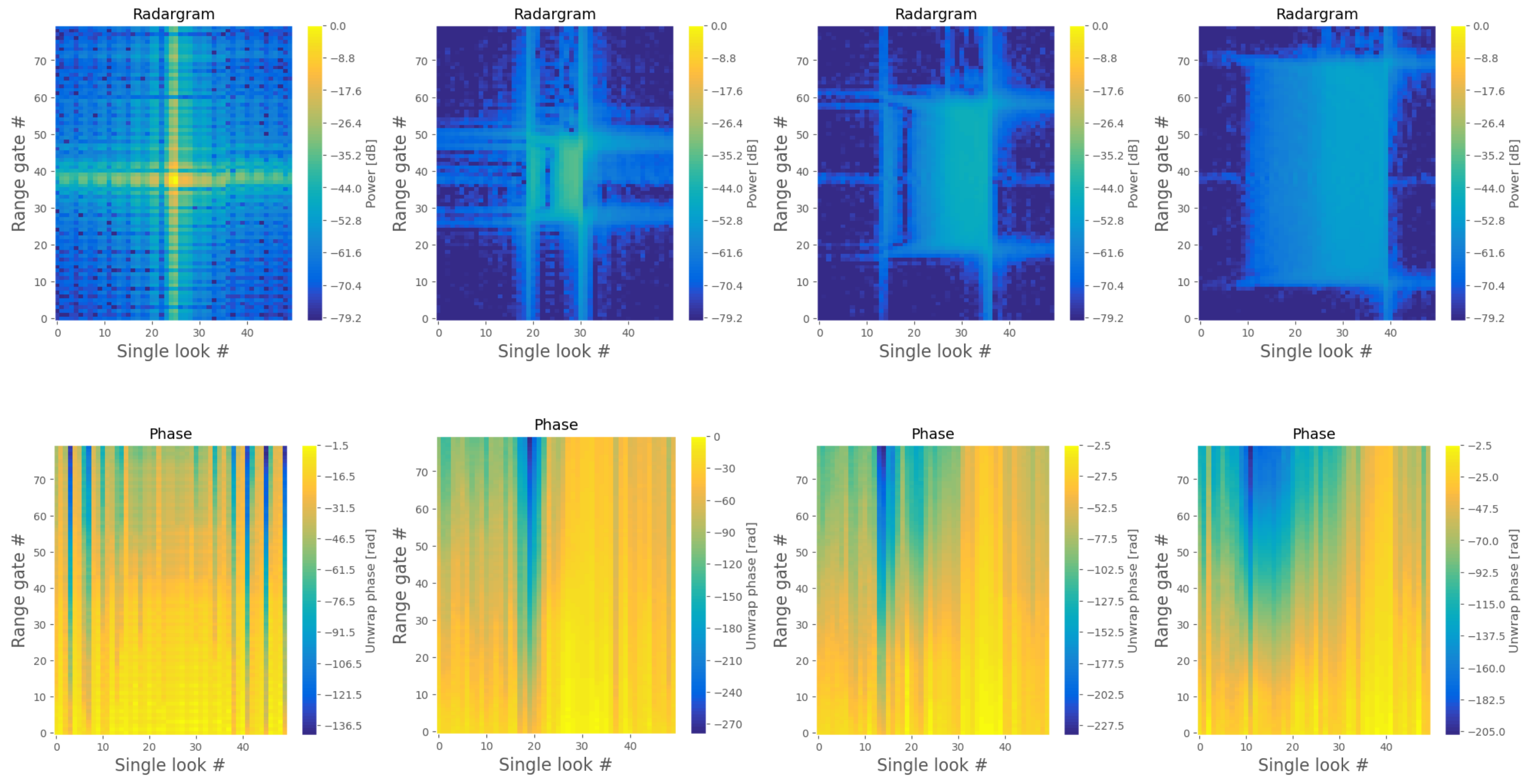
2.4. Replicas Mitigation

The problem. When data are acquired in a closed-burst configuration, as occurs for C2 and S3, the amplitude signal behaviour, represented by the chronogram $\chi$ [8], is characterized by a sequence of rectangular functions $\Pi$. This is mathematically expressed as

$${\displaystyle \chi \left(\eta \right)=\sum _n\Pi \left(\frac{\eta -n{T}_p}{T_b}\right).}$$

(9)

Here, $T_p$ is the burst repetition time, while $T_b$ is the burst duration. Although S6-MF is an open-burst altimeter, its chronogram is organized in 64 pulses at the Ku-band separated by 2 pulses: one C-band and 1 calibration pulse. Formally speaking, this organization transforms S6-MF into a closed-burst altimeter. Exploiting this signal over a duration longer than the burst leads to the emergence of what is known as grating lobes, or simply replicas. From [1] [Equation (35)], it is clear that a periodical repetition of the open-burst fully-focused impulse response exists every $1/T_p$ in the frequency domain, and is contained in the envelope of the unfocused impulse response. The amplitude A in dB of the first replica (compared to the main lobe) and its position d in meter are respectively given by:

$$A=20log\left(\left|\sin \mathrm{c}\left(\frac{T_b}{T_p}\right)\right|\right),d=\frac{v_g}{T_p\left|{\dot{f}}_d\right|}.$$

(10)

For S6-MF, this results in an approximate A value of −33 dB and a position d of around 300 m. Recent research [14,15] has highlighted the multifaceted nature of replicas, affecting both the along-track and across-track dimensions. These replicas can contaminate different range gates, resulting in a smearing effect. The complete mathematical expression of the replica model is available in Appendix B. In scenarios with low MSS, which corresponds to a drastic reduction in the integration time, the smearing takes the form of a parabola, as shown in Figure 5a. Replicas of this type, observed within a 2 s interval surrounding the primary signal, pose a particular challenge in the estimation of water surface height (WSH). The retracker, a crucial component of altimetry, is prone to the influence of replicas, particularly in the thermal noise area. This can lead to significant errors in WSH, often exceeding tens of meters, as illustrated in Figure 5b. Various retracking algorithms, including empirical (e.g., OCOG) and optimal retrackers (e.g., sinc squared), experience similar difficulties. This challenge is particularly pronounced in environments such as inland water and sea-ice regions. The heterogeneous nature of these surfaces can result in differences in amplitude (image dynamics) exceeding the −33 dB amplitude level of the first replica.

The mitigation strategy. Addressing the issue of S6-MF replicas mitigation is of high importance, especially when considering applications in areas characterized by specular surfaces. In response to this challenge, we have developed an innovative method that retains all pulses while remaining easy to implement. As described in the Appendix B, replicas are subject to a smearing effect that is stable in amplitude but not in phase, where their phase varies along the along-track direction. This phase variation is illustrated in Figure 6 over the first three replicas on the CDN1 transponder [16].

Our strategy revolves around the identification of anomalies in the radargrams, specifically focusing on opposing phase variations. To achieve this, we rely on a coherence measurement that involves N consecutive complex single-looked waveforms ${\left\{s_k\right\}}_{k=0}^{N-1}$ contained in each multi-looked waveform of index i. The coherence measurement is represented by the following equation:

$$c_i=\frac{{\left|{\sum }_{k=0}^{N-1}\left|s_k\right|exp\left(j·arg\left(s_k\right)\right)\right|}^2}{N{\sum }_{k=0}^{N-1}{\left|s_k\right|}^2}.$$

(11)

The coherence can be seen as the ratio between two multilooking techniques of individual single-looks. The first technique involves a complex summation (as found in the numerator), while the second technique involves a power summation (as evident in the denominator). When the phase among single looks remains constant, the ratio is equal to one. However, if the phase exhibits variations, leading to interference among single looks, this ratio may decrease, eventually reaching zero.

We implemented the coherence-based replicas removal strategy on FF data collected over the Garonna river surface, depicted in Figure 7. This process involved estimating the coherence of each multi-looked FF element within the radargram, leading to Figure 7b. At a frequency of 500 Hz, which represents 25 single looks contained within each multi-look, the coherence values over the Garonna river exhibit near-zero readings at the positions of the replicas. By a simple multiplication of the radargram and the coherence images, we obtain a new radargram weighted by the highly correlated consecutive single-looks. This weighted radargram, as displayed in Figure 7c, effectively eliminated the replicas, resulting in highly satisfactory retracking results. It is important to note that this approach resolves WSH estimation errors caused by replicas, all without introducing any aliasing effects. It is essential to emphasize that the replicas removal technique outlined above is exclusively applicable to the S6-MF altimeter. In contrast, for altimeters with close-burst chronograms, such as S3 or C2, the presence of phase interference among replicas cannot be compensated for by using weighting methods. In such scenarios, more sophisticated methods, including image deconvolution techniques [17], are necessitated to address this issue.

2.5. Multilooking

The main interest of multi-looking is to reduce the Gaussian distributed speckle noise, thereby improving the accuracy of geophysical parameter estimation. Unlike the incoherent processing method in UF-SAR, which involves accumulating looks from different incident angles but at the same ground location, FF-SAR multilooking performs spatial averaging. It involves averaging consecutive single-looks to reduce the impact of gamma noise. However, this approach comes at a cost—namely, the along-track spacing, which should ideally be kept as short as possible to enable high-sampling rate measurements for the detection of small targets.

The choice of the along-track spacing, or posting rate, often necessitates a trade-off between resolution and noise reduction. This trade-off is typically determined through visual observation of the waveforms. Our goal, therefore, is to establish a method that can automatically define the optimal posting rate. A higher posting rate yields a higher resolution but involves averaging fewer single waveforms, resulting in a higher noise level. This configuration is preferred for handling small water targets that require high-resolution measurement capability to distinguish them from highly reflective surrounding structures. Conversely, a lower posting rate enhances noise reduction but at the expense of resolution. This setup is better suited for application over open ocean, where the surface is larger and more homogeneous. Finding the right balance is crucial in FF-SAR multilooking.

For the sake of formalism, let us consider successive single-look FF-SAR waveforms $s_i$ with speckle noise following any random distribution with the same zero mean value, standard deviation $\sigma >0$ and a covariance factor $\rho$ that ranges between −1 and 1. When $\rho =0$, the single looks are independent, while for $\rho >0$, they are correlated, and in the special case where $\rho <0$, they are decorrelated. Let us consider the special case where the correlation factor between single-looks follows an exponential law:

$$\mathrm{cov}(s_i,s_j)={\sigma }^2{\rho }^{|j-i|},\forall i,j\in \mathbb{N}.$$

(12)

The previous equation arbitrarily models (through $\rho$) the speckle decorrelation with spatial distance between waveforms as an exponential decaying law. Multilooking consists of the average of n power waveforms and results in a reduction in variance (i.e., its power, since waveforms have null mean), as shown by the equation:

$$\frac{1}{n^2}·\mathrm{var}\left(\sum _{i=1}^n{s}_i\right)=\frac{1}{n^2}\sum _{i=1}^n\mathrm{var}\left(s_i\right)+\frac{2}{n^2}\sum _{i=1}^n\sum _{j=i+1}^n\mathrm{cov}(s_i,s_j),$$

(13)

where i and j are the indexes. By injecting (12) into (13), we can derive the final expression for the variance as follows (the double sum has been solved by using the geometric series rule):

$$\frac{1}{n^2}·\mathrm{var}\left(\sum _{i=1}^n{s}_i\right)=\frac{1}{n}{\sigma }^2+\frac{2}{n^2}{\sigma }^2\sum _{i=1}^n\sum _{j=i+1}^n{\rho }^{j-i}={\sigma }^2\left(\frac{1}{n}+\frac{2}{n^2}\frac{1-n+n\rho -{\rho }^n}{2-\rho -{\rho }^{-1}}\right).$$

(14)

The optimal multi-looking factor is determined by the number of single looks that need to be averaged to achieve a variance reduction below a specified threshold. Here, we aim to reach a minimum 80% decrease in variance, which is commonly handled by retracking algorithms based on a maximum likelihood estimator [18]. If the single looks were fully independent (i.e., $\rho =0$), the variance would decrease as $1/n$ (the black solid line in Figure 8). However, real single-look waveforms are somewhat correlated, with an estimated $\rho$ of approximately 0.5, causing the variance to decrease more slowly. Figure 8 shows that multi-looking has a slight dependence on SWH, even in the thermal noise region. To achieve a noise reduction of 80%, 65 consecutive single-looks need to be averaged for SWH around 4 m, compared to 60 for SWH around 2 m. This corresponds to a posting rate of 140 Hz and 151 Hz, respectively. For higher SWH values, the waveform gets wider in the across-track direction and contaminates the thermal noise area by injecting a correlated signal from the surface. This explains the slightly higher number of single looks required for multi-looking as SWH increases. It is also worth noting that a more substantial noise reduction would require averaging a much larger number of single looks, resulting in a significant loss of resolution.

2.6. Final Recommendation

In summary, we have classified surfaces under two categories: (a) specular, corresponding to low MSS such as rivers or sea-ice leads and (b) non-specular, corresponding to high MSS such as large lakes, open-ocean or coastal zones.

Table 2. Final recommendation of the best configuration for S6-MF FF-SAR processing. The targets are separated into two categories, specular and non-specular, with their own recommendations.

Surface Type	% of DB	Int. Time	Ant. Comp.	Windo-Wing	Replica Mit.	Multi-Looking
Specular	75%	2.55	yes	yes	yes	300–500 Hz
Non-specular	60%	2.05	yes	no	no	150–200 Hz

presents our final recommendations for FF processing parameters for these two surface types. For example, we highly recommend along-track windowing (Hamming or Gaussian) over specular areas. In contrast, it is not particularly beneficial over non-specular areas and may even result in a loss of resolution, thereby diminishing image quality. Regarding integration time and multi-looking (which affect resolution and spacing), our recommendations also vary. High resolution is crucial for specular areas to discriminate small structures effectively. However, it is not as critical for open ocean regions, where the dominant factors are speckle noise and sea surface motions.

3. Validation Based on a Synergy with Sentinel-1 Imagery

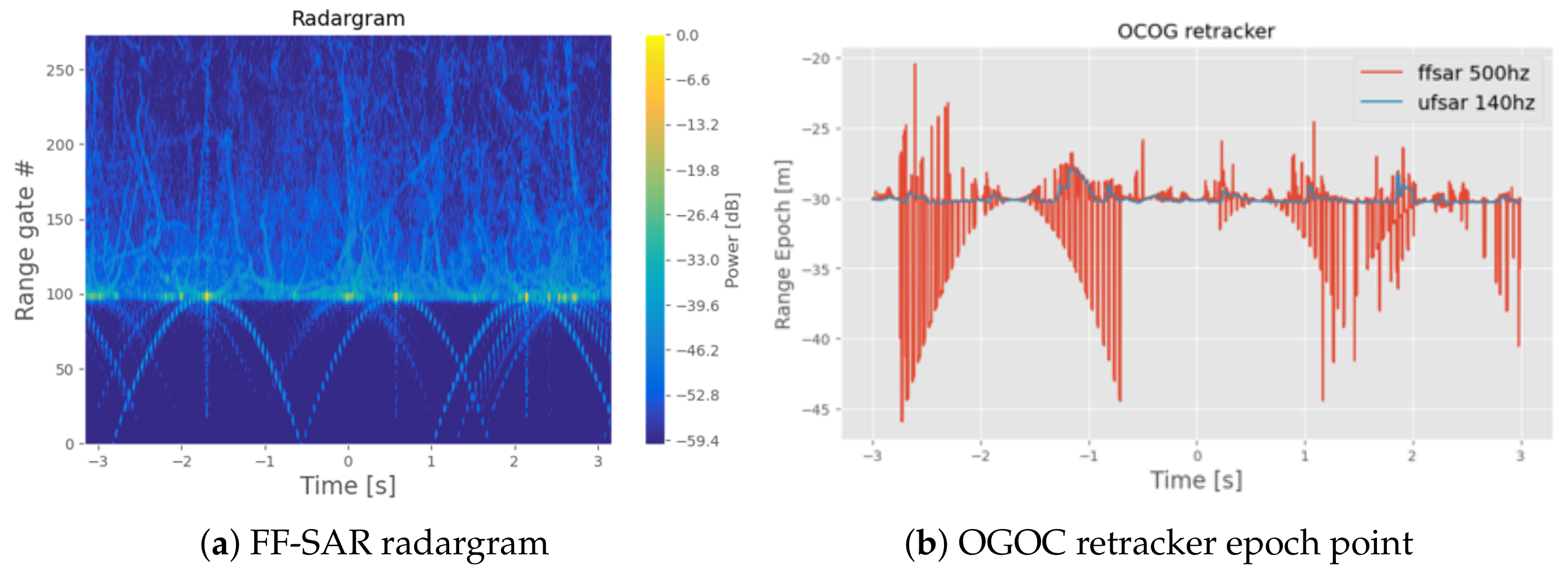
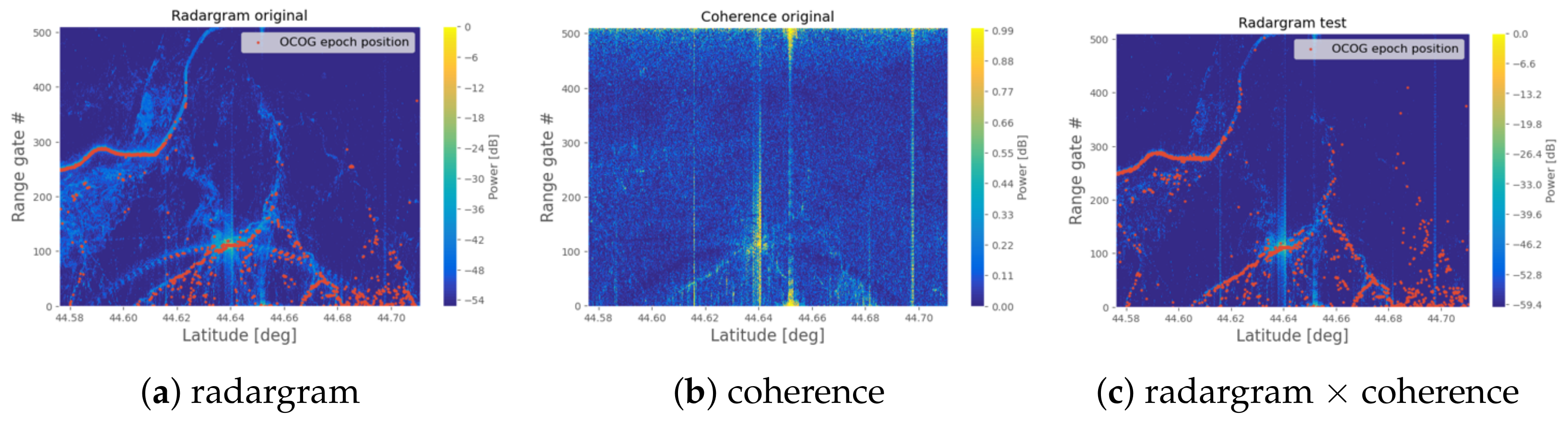
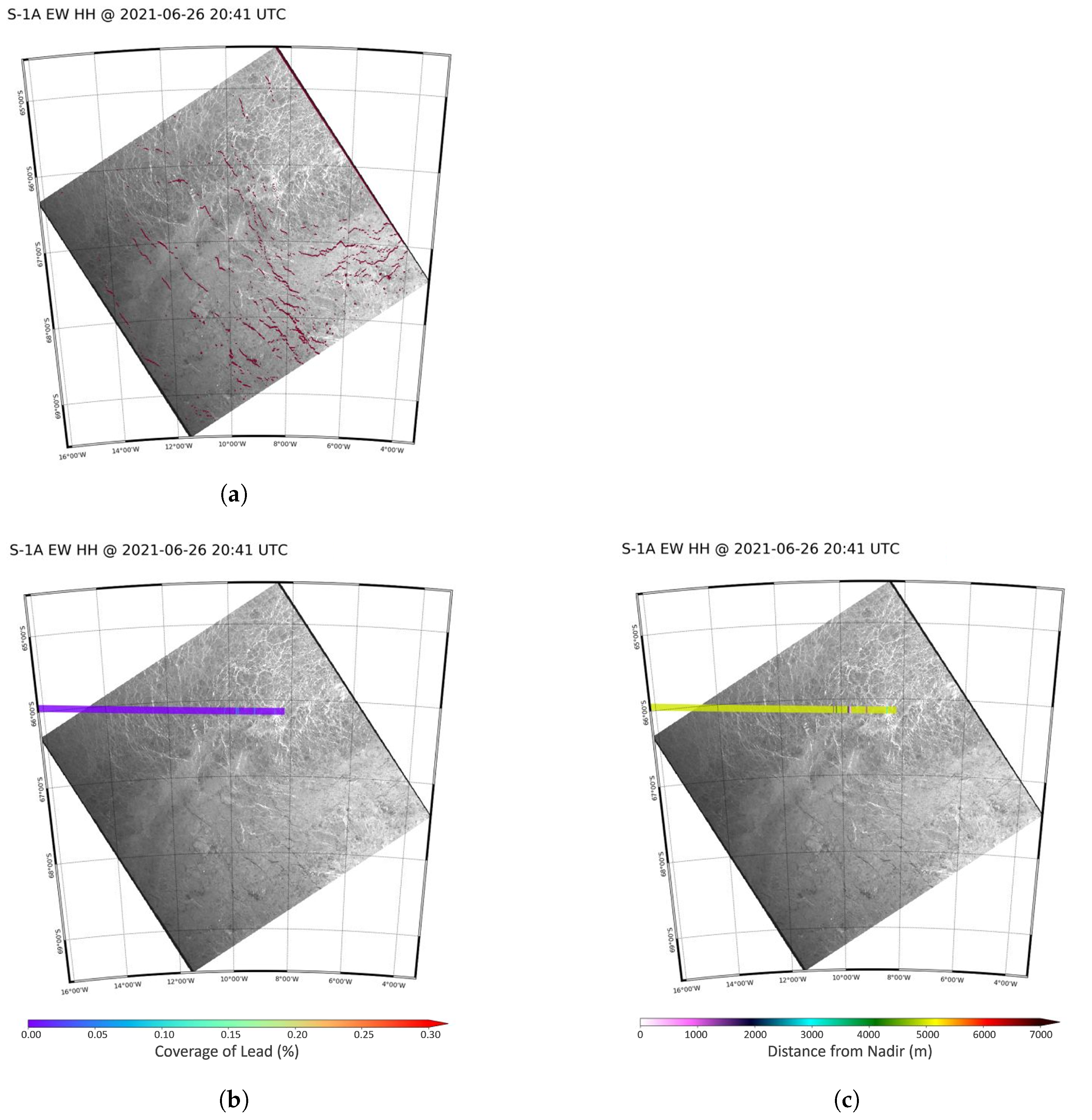
3.1. Sea-Ice Lead Detection

The first FF results have demonstrated its ability to enhance the exploitation of radar altimetry up to its finest along-track resolution. We anticipate significant improvements in identifying small, heterogeneous surface features, such as distinguishing between sea-ice leads and floes or differentiating between water and land in hydrological settings. Several studies have already been carried out to assess the FF processing performance for mapping the surface of hydrology water bodies with respect to reference water masks, but also estimating water surface elevations by comparison with in situ data [4]. However, applying this technique to sea-ice areas presents greater challenges due to the constant movement and drift of the sea-ice surface, which is driven by ocean currents and winds. No water mask is available and it is impossible to install and maintain in situ instruments at such latitudes.

In this work, we employ a unique approach to evaluate the FF altimeter’s capability to detect open waters (known as leads) within sea-ice cover. We achieve this by assessing the FF altimeter’s consistency and reliability in comparison to Sentinel-1 satellite images, as described by Longépé et al. [19], and using the following tools: (1) an updated version of the SMAP code [20] to generate the FF WK S6-MF data, and (2) the leads detector developed by Longépé et al. [19] for the identification of leads in S1 images, distinguished by their darker colour compared to the surrounding floes. The detector employs an optimal threshold-based segmentation algorithm to isolate regions with low backscatter intensities and high sea-ice concentration values. It further utilizes a morphological grayscale reconstruction algorithm to detect local minima, followed by Sobel and watershed algorithms to define the leads by flooding. We use the same threshold values as recommended by Longépé et al. [19] for Sentinel-1 backscattering (6dB) and sea-ice concentration (50%), which are relatively permissive thresholds.

Within FF radargrams, a lead can be identified by a high sigma0 level, but also by a stability in phase and amplitude between consecutive single-looks on the ground. To quantify this stability, we introduced the coherence factor in the previous section (see Equation (11)). Unlike sigma0, the coherence factor has proven to be unaffected by replicas. Given the problematic nature of replicas in sea-ice regions, we will utilize coherence to discriminate leads from floes. This will complement a common thresholding method applied to S6-MF sigma0 values. The FFSAR processing configuration aligns with the specular surface recommendations detailed in Table 2, with a multilooking level of 500 Hz, corresponding to 10 m of spacing on ground.

Finding collocated S1 and S6-MF data over sea-ice presents several challenges, chiefly due to the maximum latitude coverage of 66 degrees for S6-MF and the dynamic nature of sea-ice, which can drift at speeds of several hundred meters per hour. Despite these challenges, we were able to identify 28 S1 tiles that were collocated with S6-MF tracks in the Antarctic region. These acquisitions occurred between June and July 2021, with a maximum time difference of 15 min. This time lag minimizes the effects of sea-ice drift. Out of the 28 cases, we selected two based on specific criteria. The selection was based on the configuration of the S6-MF track on the S1 image to maximize coverage, the presence of sea-ice leads, and the size of the leads, which needed to be both wider and narrower than the S1 image resolution of 100 m. The first case corresponds to the S1A dual HH + HV polarization image 8A49 and to the S6-MF cycle/track 23/20. The second case corresponds to S1A image 5AE2 and S6-MF cycle/track 23/78. The time-lags between the S1 and S6-MF acquisitions are 1 and 3 min, respectively, allowing us to consider that the two sensors observed the same scene.

To compare the S1 and S6-MF datasets, we proceed as follows. We applied the Longépé leads detector to the S1 image. Then, we projected the S6-MF track onto the S1 image, approximating the S6-MF footprint as a rectangle with dimensions of 10 m along-track and 14 km across-track. For each footprint, we estimated the distance of the closest S1 lead to the S6-MF nadir point, as well as the percentage of S6-MF footprint occupied by S1 leads. A perfect match between S1 and S6-MF for a given S6-MF footprint with an identified lead would correspond to a distance of zero, meaning the S1 lead is located at the S6-MF nadir. As for the portion of the S6-MF footprint covered by the S1 lead, this value can vary, largely depending on the orientation of the lead relative to the S6-MF track. Given the substantial aspect ratio of the S6-MF footprint, this orientation plays a significant role.

In the first case presented in Figure 9, there is a strong alignment between the areas with detected leads in S1 and S6-MF. It is worth noting that the bottom panel of Figure 9 provides a zoomed-in view of the leads region at a longitude of 84.9 degrees. The FF-SAR detection method exhibits notable noise, as can be seen from the variation in the sigma0 profile over the identified leads (Figure 9d). This noise is expected due to the high posting rate of FF-SAR. Some points with low sigma0 and high coherence are seen outside of the green areas (representing S1 leads detected) of Figure 9d. However, by applying an additional sigma0 threshold of −170 dB, these points are filtered out, resulting in closer agreement with the S1 leads. In the region where the two methods agree, the distance between S1 lead and S6-MF nadir is below 1000 m and around 20% of the S6-MF footprint is covered by S1 leads.

In the second case presented in Figure 10, the agreement between S1 and S6-MF is less evident. Several small leads with a high coherence (≥$0.8$) and high sigma0 (≥$-170$ dB) are observed by S6-MF alone. Besides, for the unique lead detected by S1 (the green region), S6-MF detects two sharp leads instead, if one considers that each group of S6-MF points within the green region correspond to an individual lead. Given that the features in the S1 image are nearly perpendicular to the S6-MF track, it can be inferred that these are narrow leads, each a few tens of meters wide. These narrow leads are effectively invisible to S1, given its resolution of about 100 m. In summary, while the resolution of S1 can be a significant limitation for detecting leads narrower than 100 m, the choice of methodology can also be questioned. The thresholds used for detection are fixed empirically, and other methods, such as ridge detection techniques [21,22], may be more suitable for identifying small breaches in the ice.

To complement the visual inspection of the results presented in Figure 9 and Figure 10, we conducted a statistical analysis based on the Matthews correlation coefficient (MCC) indicator, defined as follows:

$$MCC=\frac{TP\times TN-FP\times FN}{{((TP+FP)\times (TP+FN)\times (TN+FP)\times (TN+FN))}^{1/2}}$$

(15)

where $TP$, $TN$, $FP$ and $FN$ represent the number of true positives, true negatives, false positives and false negatives, respectively. To be specific, $TP$ is the number of correctly detected leads by both S6-MF and S1; $TN$ is the number of correctly non-detected leads (sea ices); $FP$ is the number of leads detected by S6-MF, whereas they are detected as sea-ices by S1; $FN$ is the number of detected sea-ices by S6-MF, whereas they are detected as leads by S1. The MCC was used in the work of Longépé [19]; it provides a way to assess the general agreement between two dissimilar populations by combining the true/false positives and negatives. The MCC provides a score ranging from –1 (inverse prediction) to +1 (perfect prediction), with 0 indicating an average random prediction. In our first scenario (see Figure 9d), the Matthews coefficient is relatively high with a value of 0.68, indicating a good agreement. Specifically, S6-MF detects 27% of the leads in the sub-track, while S1 detects 39% of the leads. In the second scenario (see Figure 10d), as already discussed previously, the results are less favorable for cross-validation, and the Matthews coefficient drops to 0.05. In this case, S6-MF generally detects more leads than S1: 10% versus 5%, respectively.

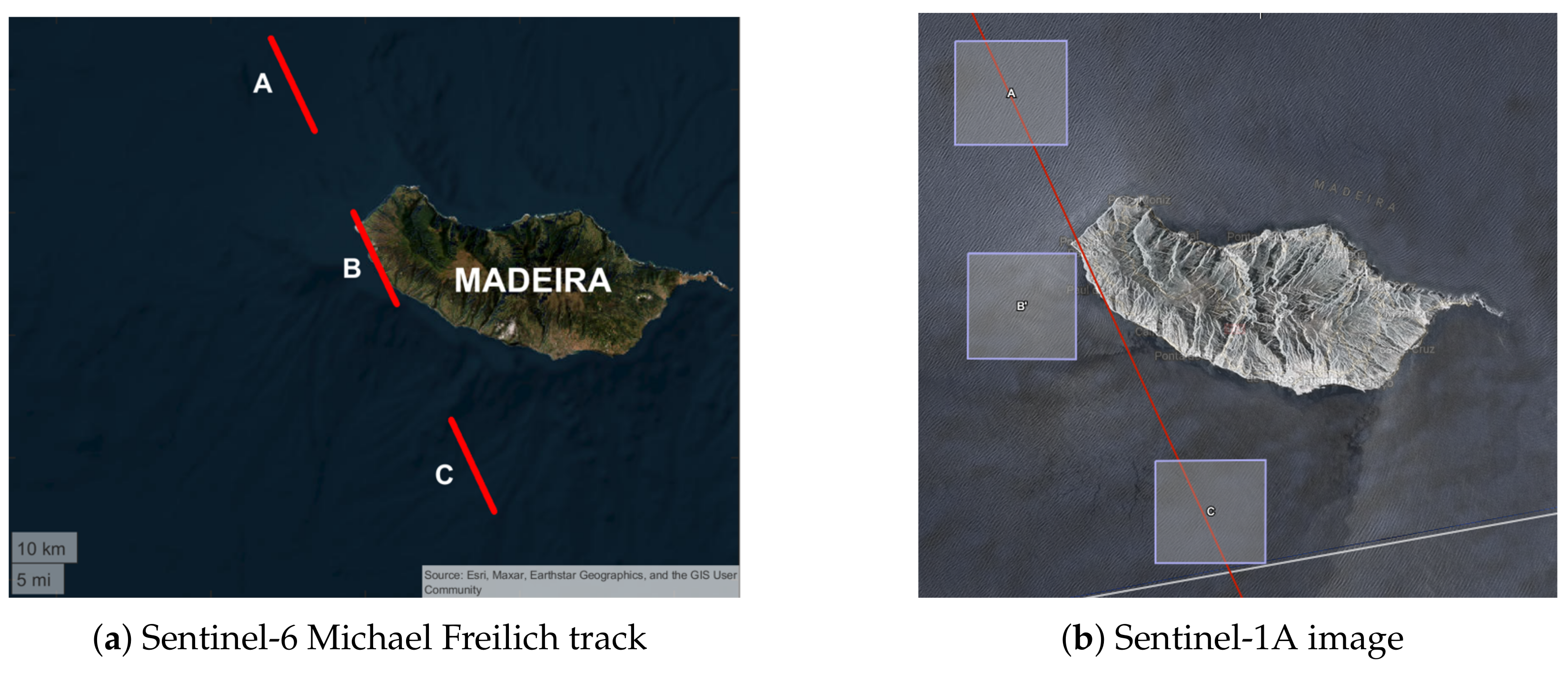
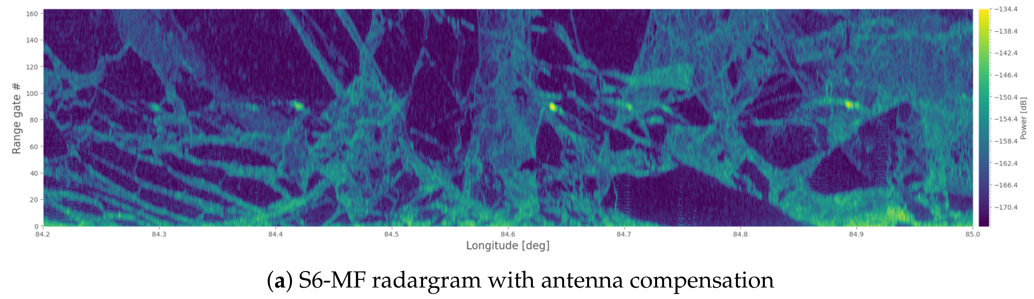
3.2. Sea-State Two-Dimensional Spectra

With the arrival of high-resolution FF radargrams, a very novel technique was developed in [6] to extract directional spectra of the ocean waves from the altimetry data for the first time. Two-dimensional spectra provide the means to monitor parameters like swell direction, amplitude, and period, as is already the case in SAR imagery. Occasionally, the superposition of mixed wave dynamics is observed, opening up the possibility to monitor complex sea-surface properties. This led to the idea of cross-validating 2D spectra from S6-MF with those from S1 over the same region.

Among all the S1-S6-MF crossing-points on the open ocean, a specific test case around Madeira Island was chosen (see Figure 11), as it stands out as a prime example in several respects. Firstly, Madeira is an island, and coastal regions are often of interest due to their dynamic complexity. Near the coast, various phenomena occur, such as wave breaking, diffraction and refraction, leading to wave groups. Secondly, coastal regions are crucial for human activities but are often poorly observed due to the hooking or adjacent effect on the measured data. Therefore, if accurate sea-state information can be provided close to the coast, it would represent a significant advancement for coastal altimetry. Lastly, due to Madeira’s topography, the issue of the left/right ambiguity, also called across-track ambiguity, may be absent. The coast has cliffs high above the ocean mean level, which implies that for a track passing near the coast, the altimeter should only receive signals from the ocean, not from the island, which should not be detected by the tracking window. This is presumably the case for zone B, which is shown in Figure 11. Directional ambiguity is especially problematic for swell direction retrieval. Altimetry, like imagery, exhibits an along-track ambiguity, artificially creating a second peak in the opposite direction of the true peak (a 180° ambiguity). However, unlike imagery, altimetry measurements cannot distinguish left and right contributions, which are summed in the radargram first and then projected onto the folded ground image, generating an additional ambiguity symmetrically regarding the the along-track direction. This means that in an FF spectra, for one true peak, we observe four peaks in different directions, while in the SAR imagery spectrum, we observe two peaks. As mentioned above, we expect that in the case of Madeira, only the along-track ambiguity remains, making it an ideal example for a cross-validation with S1.

We will not delve into the details of altimetry spectral processing, as it has already been comprehensively explained in [6]. It is, however, noteworthy to remind readers that SAR altimetry radargrams are not uniformly gridded, as the ground resolution cells (i.e., concentric annuli) corresponding to the range gates become thinner as we move away from nadir. This means that, to take advantage of the finest resolution possible, only the far-ranges’ gates are exploited. This, when combined with the FF resolution in the along-track direction, allows us to obtain a well-defined two-dimensional image. In the S6-MF mission, there is a specific mode called Range Migration Correction (RMC), which discards the first 10 and last 138 gates onboard. The mode that preserves all the range gates from 0 to 256 is known as RAW. The RMC mode is being used instead of the RAW mode to alleviate the high quantity of memory implied in the interleaved mode. Unfortunately, the S6-MF on-board processing prevents the exploitation of far range gates, potentially causing the loss of valuable sea-state information. For each FF radargram generated by the SMAP code [20], we exploit the cross-track domain from 5 to 8 km (which means a 3 km wide segment) with regards to the reference bin, i.e., the retracked bin at the leading edge. On S6-MF, the reference bin over open ocean should be around gate 55 without considering zero-padding, with a cross-track dimension going up to 14 km (in RAW mode). Conducting a dedicated sensitivity analysis to assess the impact of RAW versus RMC mode is essential. It is crucial to strike a balance between cross-track resolution and the backscattered power received, as this can affect the FF image quality. Utilizing the last range gates increases the resolution but can also result in lower backscattered power.

A large box is selected from the image or the radargram to be transformed into a 2D spectrum through Fourier transformation (see Figure 12). The size of the box is 20 × 20 km on S1 and 3 × 15 km on S6-MF, with the dimensions spanning across-track and along-track directions, respectively. Boxes A and C have been selected in such a way that they cover nearly the same ground scene (refer Figure 11b). However, this was not achievable for box B, since Figure 11b reveals that a significant portion of land covers the S1 image along the S6-MF flight direction in this region. To prevent land contamination during the computation of the S1 spectrum and ensure comparability with the S6-MF modulation spectrum, we shifted the S1 box B to the west. In the FF configuration, the chosen along-track spacing is approximately 18.8 m. We could have opted for a larger spacing, which often makes it easier to observe wave stripes, but this comes at the expense of resolution.

Figure 12 displays the resulting 2D spectra, showing an overall agreement between the two sensors, with identical peak directions and periods. The parameters of the different peaks for the three zones are provided in

Table 3. Maximum peak information from the 2D spectra of Sentinel-1A and Sentinel-6 Michael Freilich over the three areas studied, where wavelength (Lp), period (Tp) and wave direction (Dir) are extracted. The direction is provided by taking into account the 180° ambiguity.

Sensor	Area A	Area B	Area C
Sentinel-1A	Lp = 276 m	Lp = 243 m	Lp = 259 m
	Tp = 13.3 s	Tp = 12.5 s	Tp = 12.9 s
	Dir = 119°/299°	Dir = 126°/306°	Dir = 128°/308°
Sentinel-6 Michael Freilich	Lp = 271 m	Lp = 252 m	Lp = 261 m
	Tp = 13.2 s	Tp = 12.7 s	Tp = 12.9 s
	Dir = 168°/348°	Dir = 137°/317°	Dir = 137°/317°

. Zones B and C are particularly intriguing, as they reveal an additional peak in both S1 and S6-MF spectra, superimposed on the peak already present in zone A. This extra peak exhibits a slightly different period and direction compared to the main modulation signal. This phenomenon can be attributed to the impact of the coast, which distorts the waves through refraction, creating a distinct but closely related signature near the original oceanic wave. These two sea states appear to persist even as the satellite moves away from the island, as depicted in zone C. To gain a better insight into this, it would be necessary to calculate several smaller consecutive boxes along the track in order to characterize the evolution of the two sea states in the wave spectra. This could be the subject of a specific study.

As expected, the across-track ambiguity effect is evident in the S6-MF spectra over the open ocean. In zones A and C, peaks appear to the left and right of the along-track direction (indicated by the orange dashed arrow), while on zone B, swell signals are present only on one side. The peak in the direction 137° (or 317° due to the 180° ambiguity) is common to the three areas, with the same direction and period but differing amplitudes. In zones A and C, the left/right ambiguity generates additional peaks with varying amplitudes. Unlike the inherent SAR ambiguity, the left/right ambiguity often manifests as two peaks with different amplitudes. This pattern is regularly observed, though not yet fully understood. The weaker peak does not necessarily correspond to the wrong signal, as demonstrated in the Madeira example, where the lowest peak shifts from one quadrant to another in the transition from zone A to B. Consequently, these ambiguities are considered equally problematic as the 180° ambiguity. The S6-MF spectra also reveal a smearing effect which might be caused by the limited across-track resolution of the RMC mode. As mentioned earlier, to mitigate this effect, more far-range gates need to be considered.

A partitioning of swell waves in altimetry spectra has not yet been developed due to the non-linearity of the transformation from modulation spectra into wave spectra, making this process highly complex. Consequently, we limit this analysis to the comparison of peak parameters (specifically, the maximum amplitude) between S1 and S6-MF, without considering swell partitioning. The peak parameters are summarized in Table 3, confirming a good agreement between S6-MF and S1 in terms of period and wavelength. The largest differences between the two sensors are observed for zone B, with differences of 0.2 s in period and 9 m in wavelength. These values are nonetheless low, indicating a satisfactory level of agreement. In zone C, the period is exactly the same, with only a 2 m difference in wavelength. The direction is somewhat more challenging to interpret due to the left/right ambiguity, which generates attenuated peaks. In zone A, the maximum peak is at 168° (or 348°) in S6-MF, while S1 detects a wave direction of 119° (or 299°). In this case, the weaker peak is the true peak, highlighting the importance of not relying solely on maximum detection. In zones B and C, there is a better correspondence. The direction of the main peak in S6-MF is around 137° (or 317°), which is close to the S1 values of 126° (or 306°) and 128° (or 308°) for zones B and C, respectively. In summary, the unique configuration of the S6-MF track along the island’s coast, which eliminates the left/right ambiguity, illustrates the potential of S6-MF to retrieve properties of swell waves. The differences observed between S6-MF and S1 are generally small and acceptable for practical applications.

4. Discussion and Conclusions

In this paper, we demonstrate the remarkable capability of FF-SAR to observe small-scale patterns with a level of resolution never previously achieved in altimetry. When ideally configured, this new processing opens a multitude of possibilities for monitoring various types of surfaces, from the traditional open ocean to hydrology and sea-ice. To achieve this, we provide a set of parameters (integration time, Doppler bandwidth and along-track windowing) that are specifically tuned to process both specular and non-specular targets. Users can refer to the available surface flags to determine which set of parameters is most appropriate for their specific application. Additionally, we have offered recommendations concerning replica mitigation and the posting rate.

We believe that on specular targets, the windowing is an important asset to enhance the signal-to-noise ratio, even though it comes at the cost of degrading the resolution. It is worth noting that the resolution is already compromised on surfaces with anisotropic scattering characteristics, which effectively act as a natural form of windowing. As detailed in the paper, replicas are a significant concern on specular surfaces. Various strategies can be used or have been proposed to tackle this problem, from the deconvolution [23] to the identification of peak signature on a radargram [24]. However, these techniques are very challenging to implement due to the complexity of the observed scenes and the lack of information that might lead to inconsistent results. The method we have proposed, based on the complex summation of single looks, effectively removes replicas and is straightforward for users to implement. The downside of this approach is that it also removes incoherent targets in the radargram, which, like replicas, result from destructive interference between single looks.

On non-specular targets, the key point concerns the size of the frequency domain that is filled, which reveals the aliasing problem specific to the S6-MF mission. The Doppler domain, as well as the integration time, should be reduced by means of the proportional relation between time and frequency. Multilooking, which essentially reduces the speckle noise, is another essential consideration, especially for open-ocean areas. To identify wave modulation in an FF radargram, which is crucial for generating 2D spectra, a certain level of multilooking is thus needed. For 80% of noise reduction, which we consider satisfactory, we recommend to configure the posting rate between 150 Hz to 200 Hz, or equivalently in ground sampling between 46 m and 34 m. The posting rate can be selected with a higher value, but the user shall then expect a higher level of noise in the data.

The high-resolution along-track data provided by FF enables altimeter radargrams to be visualized as folded images, allowing for the application of pattern recognition techniques developed for SAR imagery. In this context, we explored the potential to detect sea-ice leads in S6-MF FF radargrams, primarily using the coherence of single-looks. The results indicate that S6-MF has the ability to detect thin leads, with sizes of less than 100 m, which are typically invisible to S1. Monitoring such leads is especially valuable during the ice transition period.

In the case of sea-ice, the FF processing, specifically through the coherence of single looks, has demonstrated the ability to identify even thinner leads than S1, which is very important during the ice transition period. A potential approach could involve applying the same lead detection algorithm used for S1 to the FF radargram directly. Similar to the coherence, the trailing edge of the signal should not be significantly affected by the presence of replicas (due to the replicas parabola shape directed towards the first range gate), allowing it to be exploited safely. This is illustrated by the results presented in Section 3, which show a good agreement between the S6-MF and S1 2D spectra, despite the extra ambiguity inherent in the altimetry spectra. The coast can be utilized to advantageously address S6-MF’s inherent left/right ambiguity. Given that coastal regions are often less well-known compared to offshore regions, this opens up exciting possibilities for coastal altimetry.

Consequently, the same philosophy of analyzing radargrams as images can be applied to sea-ice areas. Exploiting the trailing edge, which is better resolved, and treating the cropped radargram as an image, as shown in Figure 13, can reveal various structures in the floes and leads, providing valuable information about the surface in a complementary manner to the waveform retracking outputs. It is important to reiterate that, like the coherence, the trailing edge is less affected by the presence of replicas compared to the leading edge. This opens the possibility of using S1’s lead detection method on S6-MF radargrams to map sea-ice leads and their extent. To validate this new method, geo-referencing of the radargram’s range gates on the ground would be necessary for direct comparison with S1 data. This represents just one example of how altimetry can benefit from techniques and methodologies validated on other sensors, including imagery and optical data.

References

1. Egido, A.; Smith, W.H.F. Fully Focused SAR Altimetry: Theory and Applications. IEEE Trans. Geosci. Remote Sens. 2017, 55, 392–406. [Google Scholar] [CrossRef]
2. Amraoui, S.; Moreau, T.; Scagliola, M.; Guccione, P.; Alves, M.; Boy, F.; Maraldi, C.; Picot, N.; Donlon, C. Lead detection method from Sentinel-6 FF-SAR combined with imagery data, Living Planet Symposium (LPS). In Proceedings of the Meeting in Bonn, Bonn, Germany, 6–16 June 2022. [Google Scholar]
3. Egido, A.; Buchhaupt, C.; Donghui, Y.; Smith, W.H.F.; Zhang, D.; Connor, L. A Novel Physical Retracker for Sea-Ice Freeboard Determination from High Resolution SAR Altimetry, Living Planet Symposium (LPS). In Proceedings of the Meeting in Bonn, Bonn, Germany, 6–16 June 2022. [Google Scholar]
4. Gibert, F.; Gómez-Olivé, A.; McKeown, C.; Molina, R.; Garcia-Mondéjar, A. Water Elevation and Water Extent Measurements With Sentinel-6 Fully-Focussed SAR, Ocean Surface Topography Science Team (OSTST). In Proceedings of the Meeting in Venice, Venice, Italy, 27–28 October 2022. [Google Scholar]
5. Schlembach, F.; Ehlers, F.; Kleinherenbrink, M.; Passaro, M.; Dettmering, D.; Seitz, F.; Slobbe, C. Benefits of fully focused SAR altimetry to coastal wave height estimates: A case study in the North Sea. Remote Sens. Environ. 2023, 289, 113517. [Google Scholar] [CrossRef]
6. Altiparmaki, O.; Kleinherenbrink, M.; Naeije, M.; Slobbe, D.; Visser, P. SAR Altimetry Data as a New Source for Swell Monitoring. Geophys. Res. Lett. 2022, 49, e2021GL096224. [Google Scholar] [CrossRef]
7. Buchhaupt, C.; Fenoglio, L.; Becker, M.; Kusche, J. Impact of vertical water particle motions on focused SAR altimetry. Adv. Space Res. 2021, 68, 853–874. [Google Scholar] [CrossRef]
8. Guccione, P.; Scagliola, M.; Giudici, D. 2D Frequency Domain Fully Focused SAR Processing for High PRF Radar Altimeters. Remote Sens. 2018, 10, 1943. [Google Scholar] [CrossRef]
9. Phalippou, L.; Caubet, E.; Thouvenot, E. A Ka-band altimeter for future altimetry missions. In Proceedings of the IEEE 1999 International Geoscience and Remote Sensing Symposium, Hamburg, Germany, 28 June–2 July 1999; IGARSS’99 (Cat. No.99CH36293). Volume 1, pp. 503–505. [Google Scholar] [CrossRef]
10. Rostan, F.; Mallow, U. The CryoSat Earth Explorer Opportunity Mission-system calibration and mission performance. In Proceedings of the IGARSS 2001. Scanning the Present and Resolving the Future, Proceedings of the IEEE 2001 International Geoscience and Remote Sensing Symposium (Cat. No.01CH37217); Sydney, NSW, Australia, 9–13 July 2001, Volume 1, pp. 552–554. [CrossRef]
11. Donlon, C.; Cullen, R.; Giulicchi, L.; Fornari, M.; Vuilleumier, P. Copernicus Sentinel-6 Michael Freilich Satellite Mission: Overview and Preliminary in Orbit Results. In Proceedings of the 2021 IEEE International Geoscience and Remote Sensing Symposium IGARSS, Brussels, Belgium, 11–16 July 2021; pp. 7732–7735. [Google Scholar] [CrossRef]
12. Dinardo, S.; Fenoglio-Marc, L.; Becker, M.; Scharroo, R.; Fernandes, M.J.; Staneva, J.; Grayek, S.; Benveniste, J. A RIP-based SAR retracker and its application in North East Atlantic with Sentinel-3. Adv. Space Res. 2021, 68, 892–929. [Google Scholar] [CrossRef]
13. Curlander, J.C.; McDonough, N.R. Synthetic Aperture Radar: Systems and Signal Processing; Wiley Series in Remote Sensing and Image Processing; Wiley: New York, NY, USA, 1992. [Google Scholar]
14. Ray, C.; Martin-Puig, C.; Clarizia, M.; Ruffini, G.; Dinardo, S.; Gommenginger, C.; Benveniste, J. SAR Altimeter Backscattered Waveform Model. Geosci. Remote Sens. IEEE Trans. 2015, 53, 911–919. [Google Scholar] [CrossRef]
15. Ehlers, F.; Schlembach, F.; Kleinherenbrink, M.; Slobbe, C. Validity assessment of SAMOSA retracking for fully-focused SAR altimeter waveforms. Adv. Space Res. 2023, 71, 1377–1396. [Google Scholar] [CrossRef]
16. Mertikas, S.P.; Donlon, C.; Mavrocordatos, C.; Piretzidis, D.; Kokolakis, C.; Cullen, R.; Matsakis, D.; Borde, F.; Fornari, M.; Boy, F.; et al. Performance evaluation of the CDN1 altimetry Cal/Val transponder to internal and external constituents of uncertainty. Adv. Space Res. 2022, 70, 2458–2479. [Google Scholar] [CrossRef]
17. Bertero, M.; Boccacci, P. Introduction to Inverse Problems in Imaging; CRC Press: Boca Raton, FL, USA, 2020. [Google Scholar] [CrossRef]
18. Tourain, C.; Piras, F.; Ollivier, A.; Hauser, D.; Poisson, J.C.; Boy, F.; Thibaut, P.; Hermozo, L.; Tison, C. Benefits of the Adaptive Algorithm for Retracking Altimeter Nadir Echoes: Results From Simulations and CFOSAT/SWIM Observations. IEEE Trans. Geosci. Remote Sens. 2021, 59, 9927–9940. [Google Scholar] [CrossRef]
19. Longépé, N.; Thibaut, P.; Vadaine, R.; Poisson, J.C.; Guillot, A.; Boy, F.; Picot, N.; Borde, F. Comparative Evaluation of Sea Ice Lead Detection Based on SAR Imagery and Altimeter Data. IEEE Trans. Geosci. Remote Sens. 2019, 57, 4050–4061. [Google Scholar] [CrossRef]
20. Rieu, P.; Amraoui, S.; Restano, M. Standalone Multi-mission Altimetry Processor (SMAP), June 2021. Available online: https://github.com/cls-obsnadir-dev/SMAP-FFSAR (accessed on 15 February 2023).
21. Meijering, E.; Jacob, M.; Sarria, J.C.; Steiner, P.; Hirling, H.; Unser, M. Design and validation of a tool for neurite tracing and analysis in fluorescence microscopy images. Cytom. Part A 2004, 58, 167–176. [Google Scholar] [CrossRef] [PubMed]
22. Sato, Y.; Nakajima, S.; Shiraga, N.; Atsumi, H.; Yoshida, S.; Koller, T.; Gerig, G.; Kikinis, R. Three-dimensional multi-scale line filter for segmentation and visualization of curvilinear structures in medical images. Med Image Anal. 1998, 2, 143–168. [Google Scholar] [CrossRef] [PubMed]
23. Amraoui, S.; Moreau, T.; Borde, F.; Boy, F. Replica removal of FFSAR data, OSTST. In Proceedings of the Meeting in Venice, Venice, Italy, 27–28 October 2022. [Google Scholar]
24. Hernández, S.; Gibert, F.; Garcia-Mondéjar, A.; Roca, M. Leads Detection with Fully-Focused SAR in Antarctica, OSTST. In Proceedings of the Meeting in Venice, Venice, Italy, 27–28 October 2022. [Google Scholar]
Figure 1. Comparison of Doppler spectra for different integration times over (a) Gavdos transponder data (orbit cycle 042, 29 December 2021) and (b) open-ocean data (relative orbit 077, orbit cycle 002, 7 December 2020 at 14:20:01).
Remotesensing 16 01112 g001
Figure 2. Two-dimensional level-1a Sentinel-6 Michael Freilich data over different areas: transponder (a), inland water (b) and sea-ice leads (c) with various MSS observed. In along-track, the MSS is estimated for each case (df) by fitting the range integrated level-1a signal represented in dashed line. For the sea-ice example (f), two peaks are identified and fitted separately, leading to two MSS values being estimated in this area.
Remotesensing 16 01112 g002
Figure 3. Open ocean data-block with its profile in Doppler frequency before (in blue) and after (in orange) antenna pattern compensation (on the left hand side). The linear correspondence between Doppler frequency and along-track time (slow time) is also represented (on the right hand side).
Remotesensing 16 01112 g003
Figure 4. Radargram of Lot river area, France (dataset: 21 December 2020, time 17:10:28), shown using the same power dynamics and four different processing cases: (a) antenna pattern compensation, (b) Hamming window, (c) Gaussian window with σ 2 = 0.4 and (d) Gaussian window with σ 2 = 0.2 . As can be seen, the signal-to-noise ratio progressively grows from case (ad), indicating the better result achieved by the use of the Gaussian window with σ 2 = 0.2 .
Remotesensing 16 01112 g004
Figure 5. Effect of replicas over a sea-ice lead surface. Replicas (a) can be identified by their parabola-shape signature on the FF radargram. This can lead (b) to a huge difference of several meters in the estimation of the water surface height compared to those that are unfocused, since the retracker does not distinguish replicas from the real surface signal.
Remotesensing 16 01112 g005
Figure 6. Transponder FF-SAR radargram with a zoom over the main signal (first column), the first replica (second column), the second replica (third column) and the third replica (fourth column). The amplitude and phase signals are displayed in the top and bottom rows, respectively.
Remotesensing 16 01112 g006
Figure 7. Illustration of the replicas removal strategy on S6-MF over the Garonna river. The different panels show the original radargram at 500 Hz (a), the corresponding coherence (b) and the radargram multiplied by the coherence (c). The last figure corresponds to the replica removal result. The red dots show the epoch gate position from the level-2 OCOG retracker that sometimes are at replicas positions in (a), which is no longer the case in (c).
Remotesensing 16 01112 g007
Figure 8. Normalized standard deviation evolution with regards to the level of multilooking of FF single-looks. Three scenarios are plotted: theoretical decrease with independent single-looks (in black solid line), FF oceanic real data with SWH around 2m (blue solid line) and FF oceanic real data with SWH around 4m (in blue dashed line). We aim to measure the posting rate corresponding to a noise reduction of 80% represented by the horizontal black dashed line.
Remotesensing 16 01112 g008
Figure 9. Sea-ice lead observed by S1 and S6-MF in the Antarctic region on 24 December 2021 with a 1 min time lag between the two sensors. The first two rows show the S1 tile and the corresponding collocated S6-MF track, with (a) the S1 leads (in dark red) detected by the method of Longépé [19], (b) the percentage of S1 lead coverage in the S6-MF footprint and (c) the distance of the S1 lead from the S6-MF nadir (in meters). The third row is a zoom between 84.8 and 85 degrees of longitude with (d) a cross-comparison of the leads detected on S1 (represented by light green areas) versus S6-MF (represented by red dots with the sigma0 longitude profile in gray). As a reminder, a lead on S6-MF should verify two conditions: a coherence of the FF single-looks larger than 0.8 and a sigma0 of the FF multilooks larger than −170 dB. For sake of completeness in the cross-comparison, the distance to the S6-MF nadir and the percentage (here, the fraction) of the lead of the S6-MF footprint is also provided in the bottom figure. In this example, the large lead between 84.85 and 84.93 degree in longitude is seen by both sensors.
Remotesensing 16 01112 g009
Figure 10. Sea-ice lead observed by S1 and S6-MF in the Antarctic region on 26 June 2021- with 3 min time lag between the two sensors. For an explanation on how to read the subfigures (ad), see Figure 9. In this example, (d) several thin leads between −9.4 and −9.1 degrees in longitude are seen by FF-SAR on S6-MF, while S1 is able to detect only a larger one, which is certainly limited by its coarser resolution.
Remotesensing 16 01112 g010aRemotesensing 16 01112 g010b
Figure 11. The Madeira island scene overflown by S6-MF and S1A. The S6-MF track is shown in red, overlaid on (a) an image of the island and (b) the S1A image. The analysis is divided into three zones: after, over, and before the island (A, B, and C respectively). The corresponding coverage is shown by the red lines in (a) for S6-MF and by the boxes for (b) for S1A.
Remotesensing 16 01112 g011
Figure 12. Two-dimensional modulation spectra computed for S6-MF (first row) and S1A (second row). The first, second and third columns correspond, respectively, to A, B and C zones. The S1A spectra are plotted in polar grid while S6-MF spectra are in cartesian grid.
Remotesensing 16 01112 g012
Figure 13. FF radargram of a sea-ice scene captured on 24 June 2021 with Sentinel-6 Michael Freilich. The radargram is compensated from antenna pattern (a) and has been transformed into (b) by the S1 lead detector providing a classification into two categories: floes in white and leads in blue.
Remotesensing 16 01112 g013aRemotesensing 16 01112 g013b