


Noise Analysis for Unbiased Tree Diameter Estimation from Personal Laser Scanning Data

Faculty of Forestry and Wood Sciences, Czech University of Life Sciences Prague, Kamýcká 129, 165 00 Prague, Czech Republic
*
Author to whom correspondence should be addressed.
Remote Sens. 2024, 16(7), 1261; https://doi.org/10.3390/rs16071261
Submission received: 5 February 2024
/
Revised: 22 March 2024
/
Accepted: 29 March 2024
/
Published: 2 April 2024
(This article belongs to the Special Issue Biomass Remote Sensing in Forest Landscapes II)
Abstract
:Personal laser scanning devices employing Simultaneous Localization and Mapping (SLAM) technology have rightfully gained traction in various applications, including forest mensuration and inventories. This study focuses the inherent stochastic noise in SLAM data. An analysis of noise distribution is performed in GeoSLAM ZEB Horizon for point clouds of trees of two species, Norway spruce and European beech, to mitigate bias in diameter estimates. The method involved evaluating residuals of individual 3D points concerning the real tree surface model based on TLS data. The results show that the noise is not symmetrical regarding the real surface, showing significant negative difference, and moreover, the difference from zero mean significantly differs between species, with an average of −0.40 cm for spruce and −0.44 cm for beech. Furthermore, the residuals show significant dependence on the return distance between the scanner and the target and the incidence angle. An experimental comparison of RANSAC circle fitting outcomes under various configurations showed unbiased diameter estimates with extending the inlier tolerance to 5 cm with 2.5 cm asymmetry. By showing the nonvalidity of the assumption of zero mean in diameter estimation methods, the results contribute to fill a gap in the methodology of data processing with the widely utilized instrument.
1. Introduction
Accurate forest data represent an essential basis for planning and decision making [1] in sustainable forest management providing forests that serve a wide range of productive and non-productive functions [2,3]. Utilizing remotely sensed three-dimensional (3D) data obtained through multi-view photogrammetry or Light Detection And Ranging (LiDAR) offers a powerful means to assess various numerical characteristics of forest stands or individual trees [4,5]. This approach provides an efficient and objective method for acquiring forestry data supporting long term planning and operational decision-making processes. Data requirements of scientific or operational forestry applications that necessitate precise individual tree attributes can be met using close-range 3D data acquired through terrestrial remote sensing sensors [6,7] or sensors mounted on unmanned aerial vehicles (UAVs) operating at low altitudes [8], even under forest canopies [9]. Close-range 3D data typically provide detailed and accurate reconstruction of individual tree stems and crowns.
Terrestrial Laser Scanning (TLS) represents a standard 3D imaging method that provides highly detailed point clouds with millimeter-level precision [10,11], enabling accurate quantification of tree and forest parameters [12,13] or detailed descriptions of tree structures [14,15]. TLS represents an excellent tool for acquiring experimental data; however, its operational use is limited by the time-consuming process of data collection. The inability to capture trees in occlusion during scanning from a single position needs to be compensated using statistical approaches, such as occlusion corrections based on the Poisson attenuation model [16] or overcome using the time-co approach of multi-position scanning [17,18].
Mobile Laser Scanning (MLS) offers a time- and cost-effective alternative for forest data collection, enabling rapid and precise tree identification and measurement [19,20,21,22] or efficient assessment of digital terrain models [23], or quantifying forest fuel biomass [24]. MLS reduces both the occlusion effect and the time required for data collection [25] which can be up to five times faster [26] compared to TLS. Moreover, the reported tree detection rates are usually, but not exclusively [6], higher compared to TLS due to eliminating the occlusion effect [27].
SLAM-based MLS data, acquired most frequently with commercially available handheld personal laser scanning systems ZEB1 (GeoSLAM Ltd., Nottingham, UK) [26,27,28] or more recently with ZEB Horizon [19,22,29], have been in use for a relatively short time in forestry applications. Although the usefulness of MLS for forest data acquisition was confirmed by previous studies, all the methodological issues concerning data acquisition and processing have not been satisfactorily explained. Regarding data collection, it is known that the trajectory of data acquisition strongly influences the quality of acquired data [28]. However, the problem of finding the optimal trajectory in a forest environment, allowing to reconstruct efficiently the whole inventory plot or forest stand, remains to be solved.
Another significant drawback of mobile scanning is the fact that point clouds obtained using SLAM-based scanners exhibit markedly higher levels of unavoidable stochastic noise [17,21,29,30,31] caused by sensor position uncertainty [32], compared to TLS. However, SLAM technology can still provide accurate positioning of the scanner [23] which can outcompete GNSS (Global Navigation Satellite System) and IMU (Inertial Measurement Unit) positioning for forest mapping [33]. In most cases, tree stems represent features easily associable with geometric primitives’ shapes helping SLAM avoiding trajectory loss [34]. The accuracy of SLAM positioning can be affected by scene properties, such as objects or materials in the scene [35]; in forests, the accuracy may be affected especially by moving canopies or branches [34]. Although SLAM-based point clouds represent a less accurate surface reconstruction, several studies reported that the inferior surface reconstruction quality did not affect the basic tree and forest parameter estimates; the estimates derived from both MLS and TLS data achieved comparable accuracy [35], or the noisy MLS data even provided better estimates than incomplete tree surfaces in TLS affected by the occlusion effect [17,36]. Contrarywise, Fol et al. [37] reported limited ability of SLAM MLS data to quantify biodiversity measures due to the noise, and similarly the quality of SLAM MLS data may be not sufficient for accurate applications. Studies concerned with deriving tree stem diameters from SLAM data [29,35,38] show a consistent negative bias of approximately 1 cm in diameter in estimates caused by the noise distribution on tree surfaces in MLS scans.
Tree diameter in a 3D point cloud is usually assessed as the diameter of a circle or cylinder fitted to the (vertical projection of) points representing a tree cross-section of a given height using various techniques [39,40,41]. RANSAC (Random Sample Consensus) is an iterative stochastic method developed to fit a mathematical model in noisy data based on repeated model fitting to random subsamples [42]. RANSAC has been widely used for diameter estimation in close-range 3D data [43,44,45]. RANSAC is robust against noise, i.e., the circle is not affected by outlier points such as returns from branches, leaves or other vegetation. However, the noise in MLS data is not compound of outlier points, but of inlier points distributed along the real surface. Diameter estimation techniques typically assume symmetric distribution with zero mean [36].
This study is motivated by the results of studies reporting a consistent negative bias of approximately 1 cm in diameter estimates in SLAM data in comparison to TLS data. The study analyzes the geometric properties of noise in 3D reconstruction of tree stem surfaces acquired with GeoSLAM ZEB Horizon in terms of describing distributions of radial residuals of stem surface points from the real tree stem surface, and quantifies the dependence of residuals on factors such as scanning distance and angle. The results of the analysis contribute to understanding and mitigating the reported bias in tree stem diameter estimation.
2. Materials and Methods
The methodology of the study, explained in the following subsections, is visualized as a processing flowchart shown in Figure 1.
2.1. Research Area
The data acquisition was conducted within the School Forest Enterprise of the Czech University of Life Sciences, Prague, Czech Republic (49.956N, 14.794E). The study focused on the most abundant and economically significant representatives of coniferous and deciduous tree species in Central European forests: Norway spruce (Picea abies (L.) H. Karst.) and European beech (Fagus sylvatica L.).
For both species, two homogenous single-species mature even-aged stands with no understory and limited tree regeneration located on terrain with minimum slope (Figure 2b,c) were selected. In each forest stand, a square research plot of approximately 50 × 50 m was established. Table 1 shows the characteristics of the research plots including tree diameter at breast height (DBH) range and mean.
2.2. Data Acquisition
MLS data were collected using a GeoSLAM ZEB Horizon (GeoSLAM Ltd., Nottingham, UK) handheld personal laser scanner. Using ZEB Horizon, data were continuously collected during a walk along the object of interest. The starting point of the walking trajectory must be identical to the closing position and the trajectory should contain loops or revisit previously surveyed locations to rectify possible drift-induced inaccuracies. The trajectory of this study followed the double parallel-line pattern (Figure 2a) so that the area of the plot was systematically covered with approximately uniform density and all trees in the plot were covered from all sides.
TLS data were collected using a Trimble RX8 (Trimble Inc., Sunnyvale, CA, USA). The plot area was scanned from 16 positions approximately uniformly distributed along the perimeter and in the research plot. Spherical targets were deployed across the plot for the purpose of co-registration of individual scans.
2.3. Raw Data Post-Processing and Tree Cross-Sections Extraction
Raw data from the ZEB Horizon were post-processed using GeoSLAM Hub software 6.2.1. Raw TLS data were processed, and point clouds exported with Trimble RealWorks 11.1, which was subsequently utilized to co-register TLS and MLS data in a local coordinate system, using the cloud-based registration method. The registered TLS and MLS data were exported in ASPRS LAS format.
The objects of the analysis were the point representations of tree stem cross-sections. Therefore, individual tree point clouds were manually extracted and filtered in CloudCompare 2.12. Trees with incomplete stem reconstruction in either of the two datasets were manually removed from the study material, as well as trees with forked or damaged stems. All subsequent processing and analyses were performed in MATLAB R2021b (The MathWorks Inc., Natick, MA, USA). From the cleared MLS and TLS point clouds, points representing stem cross-sections in 11 different height levels were extracted. The above ground heights of the cross-sections were from 0.5 m to 2.5 m with 0.2 m spacing, and the height of the extracted cross-sections was 1 cm. As a result, the GeoSLAM noise was analyzed in 960 stem cross-sections of Norway spruce and 869 stem cross-sections of European beech.
2.4. Noise Characteristics
For each stem cross-section the perimeter model was derived as follows:
- Center coordinates of the cross-section were defined as the coordinates of the center of the circle recognized with RANSAC technique in the TLS point structure representing the cross-section’s perimeter returns. Within the RANSAC procedure, 1000 iterations of fitting the circle to the random subsample were used, searching for circle with the radius limited to the closed interval [0.025 m, 0.5 m]; points within 0.02 from the fitted circle were considered inliers;
- Positions of all cross-section perimeter points in TLS data were transformed to polar coordinates, i.e., the angle θ and the radial distance r. The angle from the cross-section center was calculated as the four-quadrant inverse tangent. The radial distance was calculated as the Euclidean distance between the point from the cross-section center point. The LOESS method was used to smooth the radial distances according to their respective azimuth (Figure 3); to ensure the required continuity of the smoothed curve, three repetitions of the point sequence were concatenated, and the smoothed values of the middle repetition were used. The resulting curve was considered a model of the cross-section perimeter.
Individual points were extracted from the ZEB cross-section representation and analyzed. Following characteristics were calculated for each ZEB point (see Figure 3d) for illustration):
- Scanner position at the time of the point return was calculated from the trajectory record using cubic interpolation based on the recorded GPS time;
- The Euclidean distance di to the respective scanner position was calculated as the norm of a difference vector between the coordinates of the return and the actual scanner position:where xr, yr are the coordinates of the laser return; xs, ys are the coordinates of the respective scanner position;
- 3.
- The point’s residual ei was defined as the radial distance of the point from the smoothed perimeter model, i.e., the distance of the point to the LOESS curve in the same azimuth from the cross-section center as the actual point. To calculate this, the radial distance ri between the point and the cross-section center was taken as:with xc, yc standing for the coordinates of the cross-section center, and the angle θ of the point respective to the cross-section center:were calculated. The residual ei was calculated as the difference between the radial distance of the point and the radial distance of the stem perimeter model in the given angle;
- 4.
- The incidence angle αi defined as the angle between the vectors scanner–cross section center and point–cross section center was calculated by:
The properties of the random compound of the ZEB point positions, i.e., the point radial residuals ei, were analyzed. Regression analyses were performed using the point residuals as the response variable, while the following characteristics served as explanatory variables: cross-section diameter, scanning distance di, vertical angle of the beam, incidence angle αi. Tree species, tree individual, layer height were used as covariates.
2.5. Analyzing the Effect of Scan Lines
The trajectory was manually divided into segments corresponding to individual scan lines, separated by rectangular vertices in the parallel-line pattern (Figure 4). Each point was associated with the corresponding trajectory segment based on the GPS time recorded in both the LAS file and the trajectory log.
To evaluate the effect of individual scan lines, a simulation study utilizing the derived stem cross-section point clouds was conducted, comparing center coordinates and radii of circles fitted to cross-section points belonging to individual scan lines with those fitted to random subsamples of all cross-section points. In the case that the scan lines are well co-registered, the circle parameters derived from the actual and the simulated scan lines point clouds are supposed to show no significant differences. Eventual significant difference between circles fitted to individual scan lines’ points and to random point subsets would indicate that each individual scan line forms a unique circle, influencing the result of diameter estimation and cross-section position based on scan line selection. The simulation study was carried out through following steps performed on each evaluated stem cross-section:
- A circle was detected using all points of the cross-section point set with the RANSAC technique. The circle center and radius were recorded;
- For each scan line that contained more than 10 points in the evaluated cross-section point set, a circle was fitted to all points acquired from the given scan line. The center point coordinates, and the radius of the fitted circle were recorded. Differences in circle radius and center coordinates from the circle parameters fitted to all cross-section points in previous step were calculated and recorded;
- For each scan line, a simulated scan line point set was created by selecting random subsamples from all cross-section points. This simulated point set matched the real point set in both quantity and angular range of the points across the cross-section. Perimeter points from individual scan lines covered different angular ranges, resulting in varying cross-section perimeter coverage. To standardize this, we categorized the perimeter points of each cross-section into eight angular sections based on the azimuth of individual points from the cross-section center. To maintain the original point counts and angular range of the scan line points, the original point counts in each of the eight angular sections were preserved in the simulated point set;
- The simulated scan line point set, mirroring the quantity and range of points as the real scan line point set, was used to fit a circle. The coordinates of the center point and the radius of the fitted circle were recorded, and differences from the circle parameters fitted to all cross-section points in step 1, were calculated, similar to the original scan line points (step 2);
- Circles fitted to point sets from individual scan lines exhibited variations compared to those fitted from all cross-section points. Generally, circles fitted on scan lines with fewer points on the cross-section perimeter showed increased variation in both position and radius. To analyze the effect of point count acquired from individual lines, scan line point sets were classified into six categories, 10–50 points, 50–100 points, … 250–300 points. Mean errors and standard deviations of errors in fitted circle position and radius were evaluated separately within these point count classes.
2.6. RANSAC Parameters
To assess the impact of the noise distribution in the cross-section perimeter points, an experiment for comparing the outcomes of RANSAC circle fitting under different configurations was performed. In RANSAC circle fitting, a minimum subsample that defines a circle, i.e., three points, is repeatedly randomly selected, and the circle is fitted to the subsample. The quality of each candidate fit is evaluated based on the ratio of inliers, which are points falling within a defined tolerance belt around the fitted circle. The width of the tolerance belt needs to be adjusted according to the data type and the expected surface reconstruction quality. E.g., for TLS data, Olofsson et al. [39] used a tolerance belt width of 2.5 cm; for diameter fitting in unmanned aerial scanning data or GeoSLAM ZEB data the tolerance was set to 2 and 3 cm, respectively [34,43]. To investigate the effect of tolerance belt width, the performance of RANSAC was evaluated with a set of 50 different tolerance belt widths, ranging from 2 mm to 100 mm in an arithmetic sequence with a 2 mm interval.
Considering the previously observed systematic underestimation of diameters in GeoSLAM data [24,34], the impact of tolerance belt asymmetry was evaluated. Asymmetry in the tolerance belt signifies shifts in both the inner (rin) and outer (rout) radius of the belt from the original symmetric layout (Figure 5). Specifically, the inner diameter is defined as rin = r − (tw/2 − ta), and the outer diameter as rout = r + tw/2 + ta, where tw stands for tolerance band width and ta for tolerance belt asymmetry. Asymmetry values from −50 mm to 50 mm with a 2 mm interval, resulting in 51 tested values, were tested.
The RANSAC algorithm was applied to all ZEB cross-section datasets for each combination of tolerance belt width and belt asymmetry. The number of iterations was consistently set at 1000. The diameters estimated by RANSAC under specific parameters were compared with diameters derived from TLS data, considered as the ground truth. The discrepancies in diameter estimations were recorded. To evaluate the suitability of each combination of tolerance width and asymmetry, the mean and root mean square error (RMSE) were calculated from all cross-sections, separately for the two species under consideration.
3. Results
3.1. Distribution of Residuals
The distribution of radial residuals in both species approaches a normal distribution, as illustrated in (Figure 6a), which displays the histogram of radial residuals along with the probability density functions (PDFs) of the fitted normal distributions. The parameters of the distributions vary between species: in the spruce dataset, the mean residual was −0.38 cm and −0.40 cm, on plots 1 and 2, respectively, whereas the beech dataset showed a mean residual of −0.46 cm and −0.43 cm on plots 3 and 4. Both means are significantly different from zero, as indicated by the confidence intervals in Table 2. The hypothesis of zero difference between mean residuals in the two species was rejected by a two-sample t-test (p-value < 10−10). This result implies that the noise in ZEB reconstruction of tree stems is not symmetrically distributed on both sides of the stem surface.
The Figure 6b shows the distribution of mean radial residuals in individual cross-sections for both species. The mean estimates of the mean radial residuals in cross-sections do not deviate significantly from the overall mean residuals, indicating that the distribution of radial residuals remains consistent throughout the trees and cross-sections of each species. The majority of cross-sections exhibited negative mean residuals, i.e., the return positions were shifted towards the center of the stem. Only 2% and 4% on plots 1 and 2, respectively, of cross-sections had the average residual positive for spruce. For beech, less than 0.5% of cross-sections had the average residuals positive on plot 3; plot 4 showed 9% of cross-sections with positive mean residuals, which is the effect of inconsistently large variability on plot 4, as visible in Figure 6 and shown in Table 2. The observed large variability in plot 4 might reflect an eventual error in co-registration of TLS and MLS clouds, or SLAM distortion. However, the mean of the distribution remains consistent with other plots. For spruce, the negative deviation is, on average, smaller than for beech.
3.2. Vertical Distribution of Residuals
Both species exhibit a similar pattern in the change of mean radial residuals and standard deviation of the residuals in cross-sections at different above-ground heights. The most significant negative deviations are observed in middle height layers, while in both lower and higher layers, these deviations decrease. For spruce, the most negative mean value occurs at 1.3 m above ground, which corresponds to the scanner height. This specific height aligns with the stem location where the laser beams’ incidence angle approaches perpendicularity. In the case of beech, the most substantial negative deviation was located at 1.9 m above ground, approximately 0.6 m above the scanner height level (Figure 7a). However, no significant trend in mean point residuals concerning the vertical angle or absolute value of the vertical angle of beams was observed in either species. Interestingly, the variability of mean radial residuals was consistently highest in the lowest layers (at 0.5 and 0.7 m above ground). Lower variability was found in the highest sections. However, it is important to note that the trend of decreasing variability with height above ground was not linear (Figure 7b).
3.3. Residuals According to Scanning Distance
Highly significant linear trends (p-values < 10−10) were identified in the dependence of radial residuals on the distance between the point and the scanner position from which the point was acquired (the return distance). In both species, the residual values tended to shift from negative averages for small distances to positive averages for larger distances (Figure 8). Specifically, in beech, the mean residual value shifted from negative to positive beyond a return distance of 29 m. For spruce, this transition occurred at a threshold distance of 56 m, which was technically the maximum distance recorded in the point cloud; only a few points were recorded from longer distance.
3.4. Residuals According to Incidence Angle
In both species, a consistent trend of increasing residuals with higher incidence angles was observed. The greater the angular deviation from the tree center to the scanner position line, the higher the average residual became, shifting from negative (−0.75 cm for spruce and −0.84 cm for beech). The trend exhibited an identical slope of 0.011 for both species. To explore if the observed trend can be attributed to the effect of return distance, returns were classified into five distance classes (see the legend in Figure 9), and separate linear models were applied for each class. The trend remained consistent across all distance classes. The charts in Figure 9 show several points with incidence angle over 90°. Such points are theoretically impossible to occur on cylindrical stems; however, they may appear in scans of irregular cross-sections.
3.5. Residuals According to Cross-Section Diameter
In the case of spruce, a significant (p-value < 10−10) trend was observed in the dependence of radial residuals on cross-section diameter. Throughout the diameter range, the mean residuals were negative, but for larger diameters, the negative deviation increased at an average rate of 0.0042 cm per one centimeter in diameter. No significant influence of cross-section diameter on residual distribution was observed with beech.
3.6. The Quality of SLAM Scan Alignment
The results of the simulation study, evaluating the co-registration quality of individual scan lines in cross-section perimeter reconstruction, are depicted in Figure 10. The charts illustrate the errors in position coordinates (x, y) and the cross-section radius, which were fitted to perimeter segments representing individual scan line point sets. These errors were defined as the deviations of the position and radius estimates from the position and radius derived from the complete TLS cross-section reconstruction. The range of errors in position and radius estimates consistently decreased with the point count in each scan: the more points were used to fit the circle and estimate the parameters, the smaller errors tended to occur. To illustrate this effect, data points in the charts, representing individual observations, are plotted against the point count in the respective scan. To characterize the errors that decreased with higher point counts, individual observations were categorized into classes according to the point counts in the respective perimeter segment (10–50, 51–100, … 251–300 points). The area chart shows the interval of mean error ± the standard deviation of errors in each point count class.
The errors and their corresponding numerical characteristics from real cross-section segments are displayed in the left part of Figure 10. The right part displays identical outcomes derived from the point cloud segments simulated by randomly assigning points to each segment, maintaining the point count and angular distribution. Except for the last point count class (251–300 points), which only contained three observations, there were no differences in errors produced with the real and simulated point segments. The cross-section parameters derived from individual scans do not exhibit higher errors than randomly generated point sets. This result indicates that individual scans are combined into a homogeneous cloud, rather than forming distinct point structures within the noise range.
3.7. RANSAC Parameters
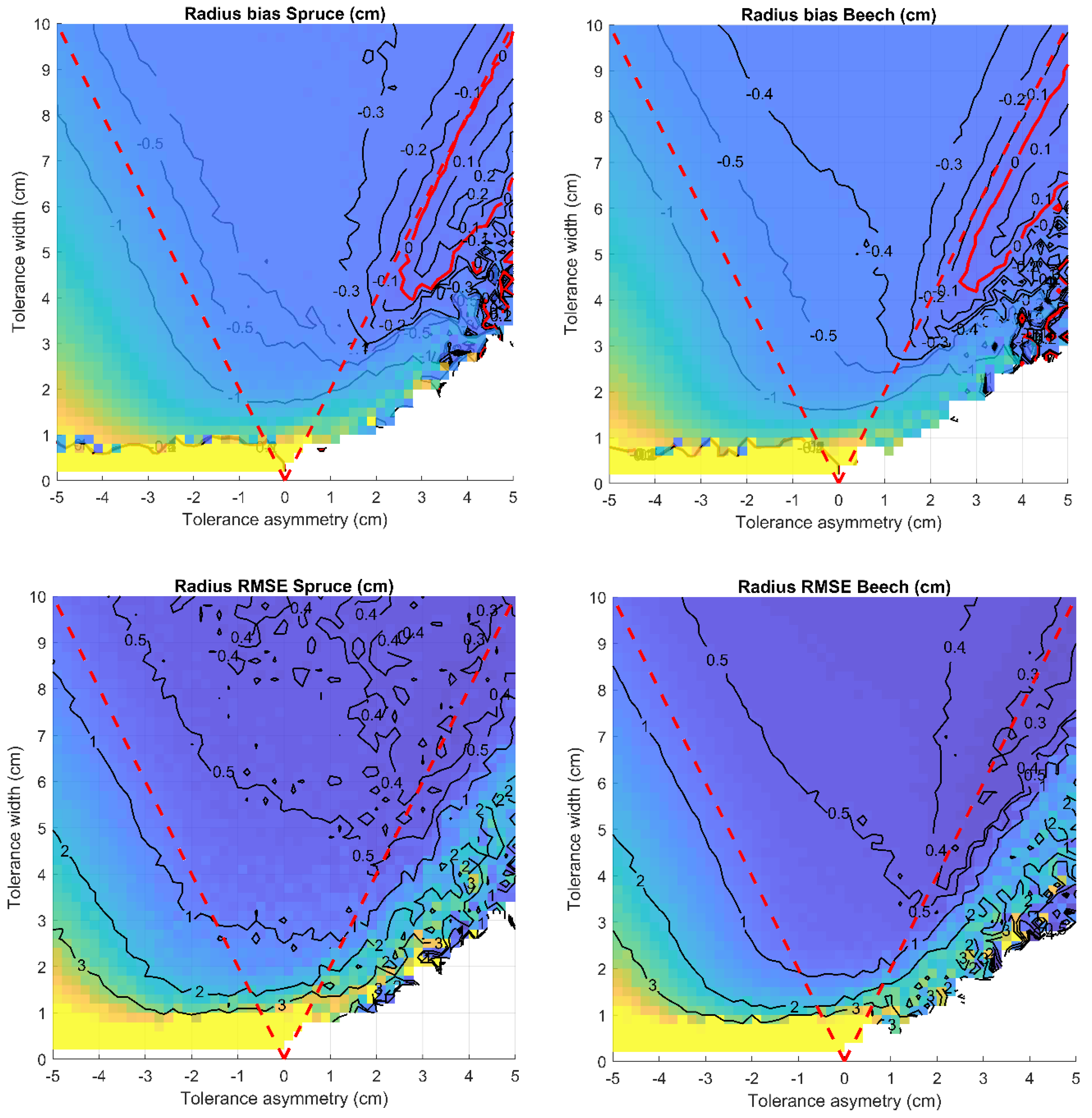
The evaluation of RANSAC parameters yielded consistent results across both species. In Figure 11, the triangular region outlined by red dashed lines represents a reasonable boundary for selecting the combination of tolerance belt width and tolerance asymmetry. Points falling outside these lines indicate scenarios where the original subsample points used for circle fitting are excluded from the tolerance belt. Excessive negative asymmetry (bottom left corner) led to increased diameter errors, while excessive positive asymmetry (bottom right corner) prevented circle generation due to insufficient inlier points. In areas beyond the red lines, large random errors lacking any discernible pattern were observed.
When the tolerance belt was symmetric (zero asymmetry applied), fitted circles consistently underestimated the diameter, with radius errors not dropping below 0.4 cm, resulting in mean diameter errors remaining above 0.8 cm. Positive asymmetry mitigated this bias. Interestingly, unbiased diameter estimates (indicated by the red contour) were achieved with asymmetry values exceeding half the tolerance belt width—essentially, tolerance belts not containing the original subsample points. For spruce, the zero-bias contour closely aligns with the red dashed line, indicating unbiased estimates when the tolerance belt touches the subsample points.
There is consistency between both indicators concerning the parameter selection. The smallest radius RMSE errors, dropping as low as 0.3 cm (equivalent to 0.6 cm in diameter), were achieved with the parameter combination ensuring zero bias. The observed relationship between errors and tolerance width, as well as asymmetry, indicates that the most accurate diameter estimates were obtained with a minimum tolerance belt width of 4 cm and an asymmetry approaching half of the tolerance belt width. The choice of tolerance width between 4 and 10 cm did not affect the accuracy of diameter estimation, provided that the asymmetry was set to the half the tolerance width.
4. Discussion
Mobile laser scanning using GeoSLAM instruments is recognized as an efficient method for close-range 3D data acquisition in forest environments, providing substantial time saving compared to TLS and easy-to-use operation compared to UAV-mounted sensors. However, data obtained through SLAM are known to exhibit noticeable noise in surface reconstruction [29,32], which must be addressed during data processing. Our study highlights that the noise is not symmetrically distributed along the reconstructed tree surface, contrary to the commonly assumed symmetric distribution in tree diameter estimation methods. This asymmetry in the noise distribution can be responsible for the observed bias in diameter estimation. Systematic underestimation of diameters in GeoSLAM data was previously reported in multiple studies [24,26,27,34]. To address this bias, Gollob et al. [24] proposed a correction function based on a linear model. The correction function can improve the diameter estimates, however, our study implies that the correction must be species-specific, since the noise distribution parameters vary between species, too. However, the underestimation of diameters can be expected as a general feature of diameter estimations for all species, as illustrated by the experiment utilizing cylindrical reference objects [24].
The presented experiment should be further elaborated with larger datasets, including more species. Additionally, more diversity in model tree diameters is needed, since the diameter estimations for trees of smaller diameters was reported to provide bias inconsistent with the larger trees [24,34]. Contrary to our results, Enrique et al. [46] report positive bias in diameter estimation on a large set of trees in a historic garden, with the bias increasing towards larger diameters. Extending the study would be required to explain such discrepancies among studies and attribute them to species-based characteristics of bark, different sensors, or different methodology.
The limitation of this experiment lies in the fact that manually cleared cross-section point representations were used. The benefit of RANSAC is the ability to eliminate the external noise, such as points originating from returns from branches and leaves, from influencing the resulting circle [39]. Our experiment does not make provision for the effect of external noise on RANSAC parameters. The results obtained on manually cleared point structures did not find the upper limit for tolerance width within the tested range 0–10 cm; the minimum errors could be obtained with any tolerance width from approx. 4–5 cm. However, the real data are likely to contain external noise even when techniques for accurate tree stem segmentation are available [47], which would limit the upper limit of tolerance width. For applications on real data, the tolerance belt width should be chosen as the lowest value that ensures minimum errors, approx. 5 cm, together with the corresponding asymmetry.
5. Conclusions
The study examined the noise present in GeoSLAM ZEB Horizon data of forest trees. The analysis involved evaluating radial residuals of individual 3D points concerning the real tree surface model based on high-quality TLS data.
As expected, residuals followed approximate normal distribution; however, what is important, the mean residual significantly deviated from zero, and this mean varied between different tree species. Specifically, Norway spruce exhibited a mean residual of −0.40 cm, whereas European beech had a mean residual of −0.44 cm. The standard deviations were around 1.4 cm for spruce and 1.5 cm for beech. Furthermore, the residuals were influenced by several factors, including return distance (the distance between the scanner and the point), angular distance to the line connecting the scanner and tree center, and aboveground height. The two species differed in the effect of diameter on radial residuals. While spruce exhibited a gradual increase in radial residuals with larger diameters, no such effect was observed with beech.
The results also show that the quality of tree surface reconstruction is not affected by the number or arrangement of trajectory passings along the tree. The composite cloud of individual scans, co-registered through the SLAM algorithm, maintains a high-quality representation of tree surface points, regardless of the trajectory configuration.
Drawing from our experimental comparison of RANSAC circle fitting outcomes under various configurations, our study offers practical recommendations for obtaining unbiased diameter estimates. It was found that RANSAC produced unbiased diameter estimations when using a tolerance belt width of 5 cm or wider, coupled with a positive tolerance asymmetry reaching its maximum value while retaining the original subsample points as inliers. Due to concerns about potential negative effects of external noise with wider tolerance belts, our study suggests that a 5 cm tolerance belt width, combined with a 2.5 cm asymmetry, yields optimal results for Norway spruce and European beech species. These specific settings are advised to achieve accurate and unbiased diameter estimates in practical applications.
Author Contributions
Conceptualization, K.K. and P.S.; methodology, K.K.; software, K.K.; investigation, K.K.; writing—original draft preparation, K.K.; writing—review and editing, P.S.; funding acquisition, P.S. All authors have read and agreed to the published version of the manuscript.
Funding
This research was funded by the Technological Agency of the Czech Republic through program CHIST-ERA, grant number TH74010001, and by the Faculty of Forestry and Wood Sciences, Czech University of Life Sciences Prague, grant FORESTin3D.
Data Availability Statement
Due to the extensive storage requirements, data are available upon request.
Conflicts of Interest
The authors declare no conflicts of interest. The funders had no role in the design of the study; in the collection, analyses, or interpretation of data; in the writing of the manuscript; or in the decision to publish the results.
References
- FAO. Voluntary Guidelines on National Forest Monitoring; Food and Agriculture Organization of the United Nations: Rome, Italy, 2017; ISBN 9789251096192. [Google Scholar]
- Díaz, S.; Pascual, U.; Stenseke, M.; Martín-López, B.; Watson, R.T.; Molnár, Z.; Hill, R.; Chan, K.M.A.; Baste, I.A.; Brauman, K.A.; et al. Assessing Nature’s Contributions to People. Science 2018, 359, 270–272. [Google Scholar] [CrossRef] [PubMed]
- Gamfeldt, L.; Snäll, T.; Bagchi, R.; Jonsson, M.; Gustafsson, L.; Kjellander, P.; Ruiz-Jaen, M.C.; Fröberg, M.; Stendahl, J.; Philipson, C.D.; et al. Higher Levels of Multiple Ecosystem Services Are Found in Forests with More Tree Species. Nat. Commun. 2013, 4, 1340. [Google Scholar] [CrossRef] [PubMed]
- Coops, N.C.; Tompalski, P.; Goodbody, T.R.H.; Queinnec, M.; Luther, J.E.; Bolton, D.K.; White, J.C.; Wulder, M.A.; van Lier, O.R.; Hermosilla, T. Modelling Lidar-Derived Estimates of Forest Attributes over Space and Time: A Review of Approaches and Future Trends. Remote Sens. Environ. 2021, 260, 112477. [Google Scholar] [CrossRef]
- Iglhaut, J.; Cabo, C.; Puliti, S.; Piermattei, L.; O’Connor, J.; Rosette, J. Structure from Motion Photogrammetry in Forestry: A Review. Curr. For. Rep. 2019, 5, 155–168. [Google Scholar] [CrossRef]
- Kükenbrink, D.; Marty, M.; Bösch, R.; Ginzler, C. Benchmarking Laser Scanning and Terrestrial Photogrammetry to Extract Forest Inventory Parameters in a Complex Temperate Forest. Int. J. Appl. Earth Obs. Geoinf. 2022, 113, 1569–8432. [Google Scholar] [CrossRef]
- McGlade, J.; Wallace, L.; Reinke, K.; Jones, S. The Potential of Low-Cost 3D Imaging Technologies for Forestry Applications: Setting a Research Agenda for Low-Cost Remote Sensing Inventory Tasks. Forests 2022, 13, 204. [Google Scholar] [CrossRef]
- Bruggisser, M.; Hollaus, M.; Otepka, J.; Pfeifer, N. Influence of ULS Acquisition Characteristics on Tree Stem Parameter Estimation. ISPRS J. Photogramm. Remote Sens. 2020, 168, 28–40. [Google Scholar] [CrossRef]
- Hyyppä, E.; Hyyppä, J.; Hakala, T.; Kukko, A.; Wulder, M.A.; White, J.C.; Pyörälä, J.; Yu, X.; Wang, Y.; Virtanen, J.P.; et al. Under-Canopy UAV Laser Scanning for Accurate Forest Field Measurements. ISPRS J. Photogramm. Remote Sens. 2020, 164, 41–60. [Google Scholar] [CrossRef]
- Liang, X.; Kankare, V.; Hyyppä, J.; Wang, Y.; Kukko, A.; Haggrén, H.; Yu, X.; Kaartinen, H.; Jaakkola, A.; Guan, F.; et al. Terrestrial Laser Scanning in Forest Inventories. ISPRS J. Photogramm. Remote Sens. 2016, 115, 63–77. [Google Scholar] [CrossRef]
- Liang, X.; Hyyppä, J.; Kaartinen, H.; Lehtomäki, M.; Pyörälä, J.; Pfeifer, N.; Holopainen, M.; Brolly, G.; Francesco, P.; Hackenberg, J.; et al. International Benchmarking of Terrestrial Laser Scanning Approaches for Forest Inventories. ISPRS J. Photogramm. Remote Sens. 2018, 144, 137–179. [Google Scholar] [CrossRef]
- Calders, K.; Adams, J.; Armston, J.; Bartholomeus, H.; Bauwens, S.; Bentley, L.P.; Chave, J.; Danson, F.M.; Demol, M.; Disney, M.; et al. Terrestrial Laser Scanning in Forest Ecology: Expanding the Horizon. Remote Sens. Environ. 2020, 251, 112102. [Google Scholar] [CrossRef]
- Wilkes, P.; Lau, A.; Disney, M.; Calders, K.; Burt, A.; de Tanago, J.G.; Bartholomeus, H.; Brede, B.; Herold, M. Data Acquisition Considerations for Terrestrial Laser Scanning of Forest Plots. Remote Sens. Environ. 2017, 196, 140–153. [Google Scholar] [CrossRef]
- Bogdanovich, E.; Perez-Priego, O.; El-Madany, T.S.; Guderle, M.; Pacheco-Labrador, J.; Levick, S.R.; Moreno, G.; Carrara, A.; Pilar Martín, M.; Migliavacca, M. Using Terrestrial Laser Scanning for Characterizing Tree Structural Parameters and Their Changes under Different Management in a Mediterranean Open Woodland. For. Ecol. Manag. 2021, 486, 118945. [Google Scholar] [CrossRef]
- Wang, D.; Liang, X.; Mofack, G.I.; Martin-Ducup, O. Individual Tree Extraction from Terrestrial Laser Scanning Data via Graph Pathing. For. Ecosyst. 2021, 8, 67. [Google Scholar] [CrossRef]
- Molina-Valero, J.A.; Martínez-Calvo, A.; Ginzo Villamayor, M.J.; Novo Pérez, M.A.; Álvarez-González, J.G.; Montes, F.; Pérez-Cruzado, C. Operationalizing the Use of TLS in Forest Inventories: The R Package FORTLS. Environ. Model. Softw. 2022, 150, 105337. [Google Scholar] [CrossRef]
- Bauwens, S.; Bartholomeus, H.; Calders, K.; Lejeune, P. Forest Inventory with Terrestrial LiDAR: A Comparison of Static and Hand-Held Mobile Laser Scanning. Forests 2016, 7, 127. [Google Scholar] [CrossRef]
- Gollob, C.; Ritter, T.; Wassermann, C.; Nothdurft, A. Influence of Scanner Position and Plot Size on the Accuracy of Tree Detection and Diameter Estimation Using Terrestrial Laser Scanning on Forest Inventory Plots. Remote Sens. 2019, 11, 1602. [Google Scholar] [CrossRef]
- Chudá, J.; Výbošťok, J.; Tomaštík, J.; Chudý, F.; Tunák, D.; Skladan, M.; Tuček, J.; Mokroš, M. Prompt Mapping Tree Positions with Handheld Mobile Scanners Based on SLAM Technology. Land 2024, 13, 93. [Google Scholar] [CrossRef]
- Solares-Canal, A.; Alonso, L.; Picos, J.; Armesto, J. Automatic Tree Detection and Attribute Characterization Using Portable Terrestrial Lidar. Trees–Struct. Funct. 2023, 37, 963–979. [Google Scholar] [CrossRef]
- Chen, S.; Liu, H.; Feng, Z.; Shen, C.; Chen, P. Applicability of Personal Laser Scanning in Forestry Inventory. PLoS ONE 2019, 14, e0211392. [Google Scholar] [CrossRef]
- Mokroš, M.; Mikita, T.; Singh, A.; Tomaštík, J.; Chudá, J.; Wężyk, P.; Kuželka, K.; Surový, P.; Klimánek, M.; Zięba-Kulawik, K.; et al. Novel Low-Cost Mobile Mapping Systems for Forest Inventories as Terrestrial Laser Scanning Alternatives. Int. J. Appl. Earth Obs. Geoinf. 2021, 104, 102512. [Google Scholar] [CrossRef]
- Muhojoki, J.; Hakala, T.; Kukko, A.; Kaartinen, H.; Hyyppä, J. Comparing Positioning Accuracy of Mobile Laser Scanning Systems under a Forest Canopy. Sci. Remote Sens. 2024, 9, 100121. [Google Scholar] [CrossRef]
- Hoffrén, R.; Lamelas, M.T.; Riva, J. de la Evaluation of Handheld Mobile Laser Scanner Systems for the Definition of Fuel Types in Structurally Complex Mediterranean Forest Stands. Fire 2024, 7, 59. [Google Scholar] [CrossRef]
- Balenović, I.; Liang, X.; Jurjević, L.; Hyyppä, J.; Seletković, A.; Kukko, A. Hand-Held Personal Laser Scanning–Current Status and Perspectives for Forest Inventory Application. Croat. J. For. Eng. 2020, 42, 165–183. [Google Scholar] [CrossRef]
- Stal, C.; Verbeurgt, J.; De Sloover, L.; De Wulf, A. Assessment of Handheld Mobile Terrestrial Laser Scanning for Estimating Tree Parameters. J. For. Res. 2021, 32, 1503–1513. [Google Scholar] [CrossRef]
- Oveland, I.; Hauglin, M.; Giannetti, F.; Kjørsvik, N.S.; Gobakken, T. Comparing Three Different Ground Based Laser Scanning Methods for Tree Stem Detection. Remote Sens. 2018, 10, 538. [Google Scholar] [CrossRef]
- Del Perugia, B.; Giannetti, F.; Chirici, G.; Travaglini, D. Influence of Scan Density on the Estimation of Single-Tree Attributes by Hand-Held Mobile Laser Scanning. Forests 2019, 10, 277. [Google Scholar] [CrossRef]
- Hyyppä, E.; Yu, X.; Kaartinen, H.; Hakala, T.; Kukko, A.; Vastaranta, M.; Hyyppä, J. Comparison of Backpack, Handheld, under-Canopy UAV, and above-Canopy UAV Laser Scanning for Field Reference Data Collection in Boreal Forests. Remote Sens. 2020, 12, 3327. [Google Scholar] [CrossRef]
- Giannetti, F.; Puletti, N.; Quatrini, V.; Travaglini, D.; Bottalico, F.; Corona, P.; Chirici, G. Integrating Terrestrial and Airborne Laser Scanning for the Assessment of Single-Tree Attributes in Mediterranean Forest Stands. Eur. J. Remote Sens. 2018, 51, 795–807. [Google Scholar] [CrossRef]
- Liu, L.; Zhang, A.; Xiao, S.; Hu, S.; He, N.; Pang, H.; Zhang, X.; Yang, S. Single Tree Segmentation and Diameter at Breast Height Estimation with Mobile LiDAR. IEEE Access 2021, 9, 24314–24325. [Google Scholar] [CrossRef]
- Ahmed, M.F.; Masood, K.; Fremont, V.; Fantoni, I. Active SLAM: A Review on Last Decade. Sensors 2023, 23, 8097. [Google Scholar] [CrossRef] [PubMed]
- Tang, J.; Chen, Y.; Kukko, A.; Kaartinen, H.; Jaakkola, A.; Khoramshahi, E.; Hakala, T.; Hyyppä, J.; Holopainen, M.; Hyyppä, H. SLAM-Aided Stem Mapping for Forest Inventory with Small-Footprint Mobile LiDAR. Forests 2015, 6, 4588–4606. [Google Scholar] [CrossRef]
- Di Stefano, F.; Chiappini, S.; Gorreja, A.; Balestra, M.; Pierdicca, R. Mobile 3D Scan LiDAR: A Literature Review. Geomat. Nat. Hazards Risk 2021, 12, 2387–2429. [Google Scholar] [CrossRef]
- Liu, K.; Xiao, A.; Huang, J.; Cui, K.; Xing, Y.; Lu, S. D-LC-Nets: Robust Denoising and Loop Closing Networks for LiDAR SLAM in Complicated Circumstances with Noisy Point Clouds. In Proceedings of the IEEE International Conference on Intelligent Robots and Systems, Kyoto, Japan, 23–27 October 2022; pp. 12212–12218. [Google Scholar] [CrossRef]
- Gollob, C.; Ritter, T.; Nothdurft, A. Forest Inventory with Long Range and High-Speed Personal Laser Scanning (PLS) and Simultaneous Localization and Mapping (SLAM) Technology. Remote Sens. 2020, 12, 1509. [Google Scholar] [CrossRef]
- Fol, C.R.; Kükenbrink, D.; Rehush, N.; Murtiyoso, A.; Griess, V.C. Evaluating State-of-the-Art 3D Scanning Methods for Stem-Level Biodiversity Inventories in Forests. Int. J. Appl. Earth Obs. Geoinf. 2023, 122, 103396. [Google Scholar] [CrossRef]
- Kuželka, K.; Marušák, R.; Surový, P. Inventory of Close-to-Nature Forest Stands Using Terrestrial Mobile Laser Scanning. Int. J. Appl. Earth Obs. Geoinf. 2022, 115, 103104. [Google Scholar] [CrossRef]
- Cabo, C.; Ordoñez, C.; García-Cortés, S.; Martínez, J. An Algorithm for Automatic Detection of Pole-like Street Furniture Objects from Mobile Laser Scanner Point Clouds. ISPRS J. Photogramm. Remote Sens. 2014, 87, 47–56. [Google Scholar] [CrossRef]
- Trochta, J.; Kruček, M.; Vrška, T.; Král, K. 3D Forest: An Application for Descriptions of Three-Dimensional Forest Structures Using Terrestrial LiDAR. PLoS ONE 2017, 12, e0176871. [Google Scholar] [CrossRef] [PubMed]
- Nurunnabi, A.; Sadahiro, Y.; Lindenbergh, R. Robust Cylinder Fitting in Three-Dimensional Point Cloud Data. Int. Arch. Photogramm. Remote Sens. Spat. Inf. Sci.–ISPRS Arch. 2017, 42, 63–70. [Google Scholar] [CrossRef]
- Fischler, M.A.; Bolles, R.C. Random Sample Consensus. Commun. ACM 1981, 24, 381–395. [Google Scholar] [CrossRef]
- Puliti, S.; Breidenbach, J.; Astrup, R. Estimation of Forest Growing Stock Volume with UAV Laser Scanning Data: Can It Be Done without Field Data? Remote Sens. 2020, 12, 1245. [Google Scholar] [CrossRef]
- Singh, A.; Kushwaha, S.K.P.; Nandy, S.; Padalia, H. An Approach for Tree Volume Estimation Using RANSAC and RHT Algorithms from TLS Dataset. Appl. Geomat. 2022, 14, 785–794. [Google Scholar] [CrossRef]
- Su, Z.; Li, S.; Liu, H.; Liu, Y. Extracting Wood Point Cloud of Individual Trees Based on Geometric Features. IEEE Geosci. Remote Sens. Lett. 2019, 16, 1294–1298. [Google Scholar] [CrossRef]
- Enrique, P.; Herrero-Tejedor, T. Assessment of Tree Diameter Estimation Methods from Mobile Laser Scanning in a Historic Garden. Forests 2021, 12, 1013. [Google Scholar] [CrossRef]
- Kaijaluoto, R.; Kukko, A.; El Issaoui, A.; Hyyppä, J.; Kaartinen, H. Semantic Segmentation of Point Cloud Data Using Raw Laser Scanner Measurements and Deep Neural Networks. ISPRS Open J. Photogramm. Remote Sens. 2022, 3, 100011. [Google Scholar] [CrossRef]
Figure 1.
The workflow of the study methodology.
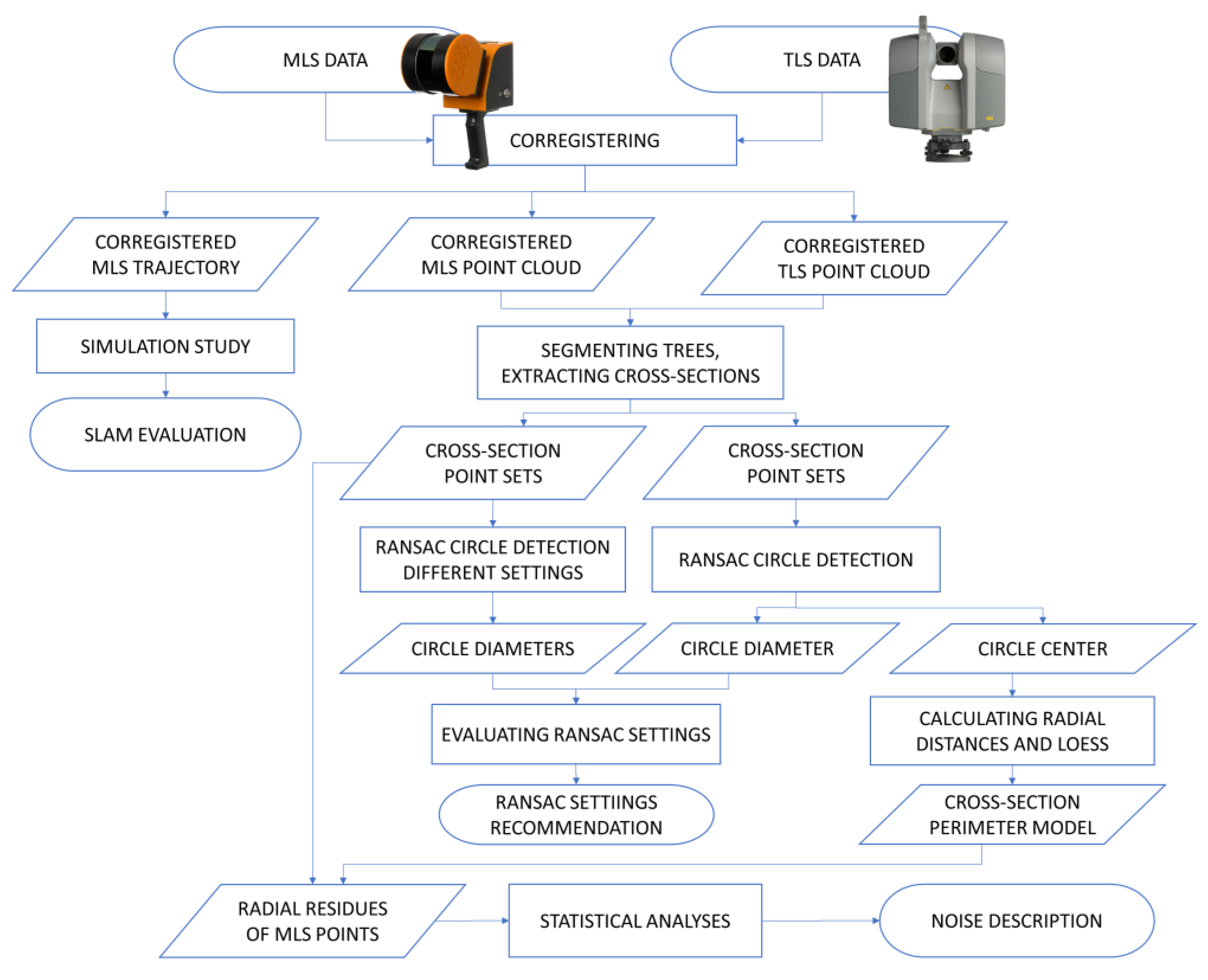
Figure 2.
(a) The trajectory of MLS data acquisition and the TLS positions in plot 1 (Norway spruce). The figure also shows the vertical projection of a TLS point cloud layer 1.25–1.35 m above ground; (b) plot 1 (Norway spruce); (c) plot 2 (European beech).
Figure 2.
(a) The trajectory of MLS data acquisition and the TLS positions in plot 1 (Norway spruce). The figure also shows the vertical projection of a TLS point cloud layer 1.25–1.35 m above ground; (b) plot 1 (Norway spruce); (c) plot 2 (European beech).
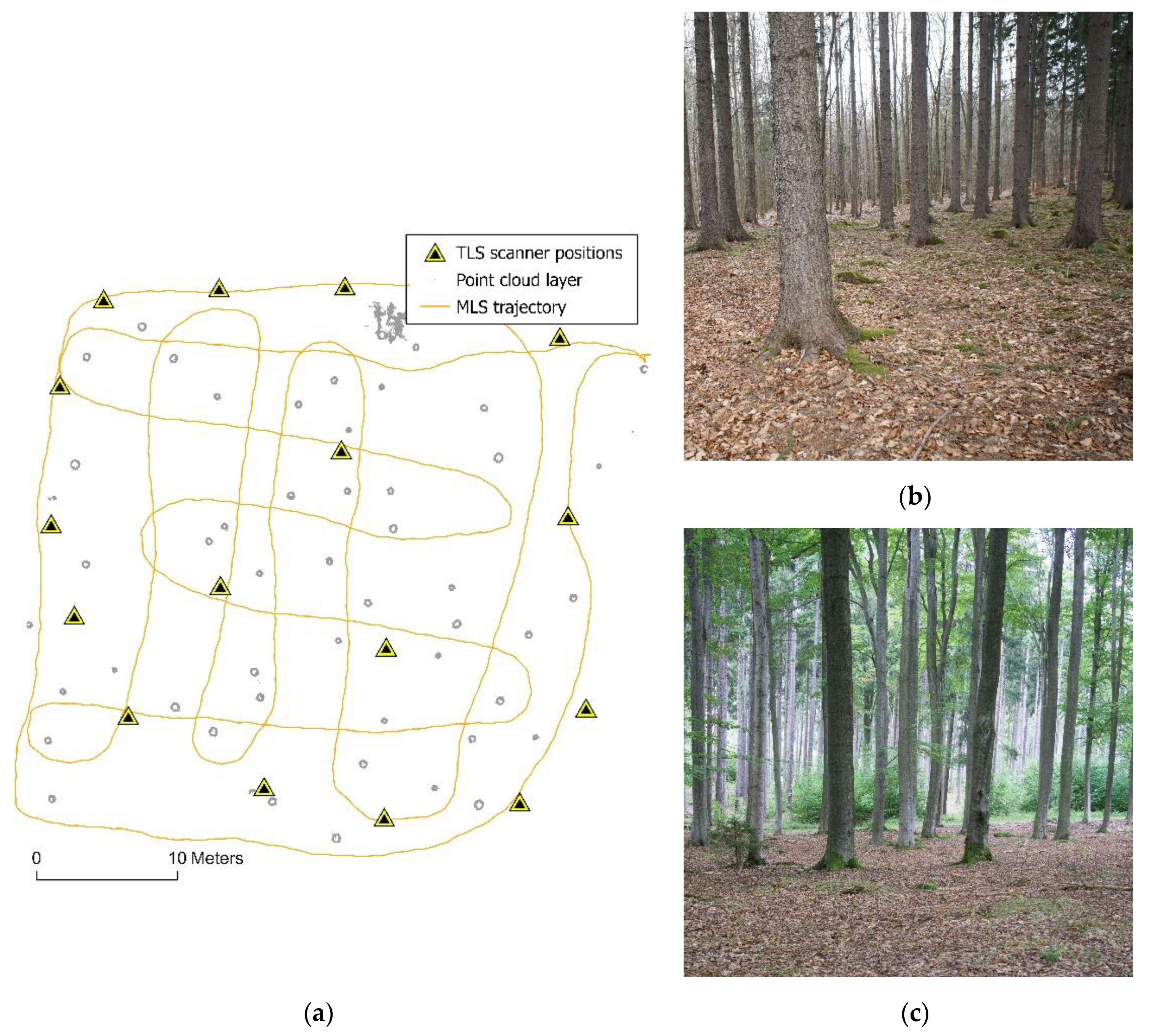
Figure 3.
Point representation of a tree stem cross-section: (a) TLS data fitted with the stem cross-section perimeter model, (b) TLS points and the perimeter model displayed as the angle and the radial distance, (c) the ZEB points with the perimeter model fitted to TLS data displayed as the angle and the radial distance, and (d) the ZEB points with the perimeter model, and the explanation of return distance (di), incidence angle (αi), and the radial residual value (ei).
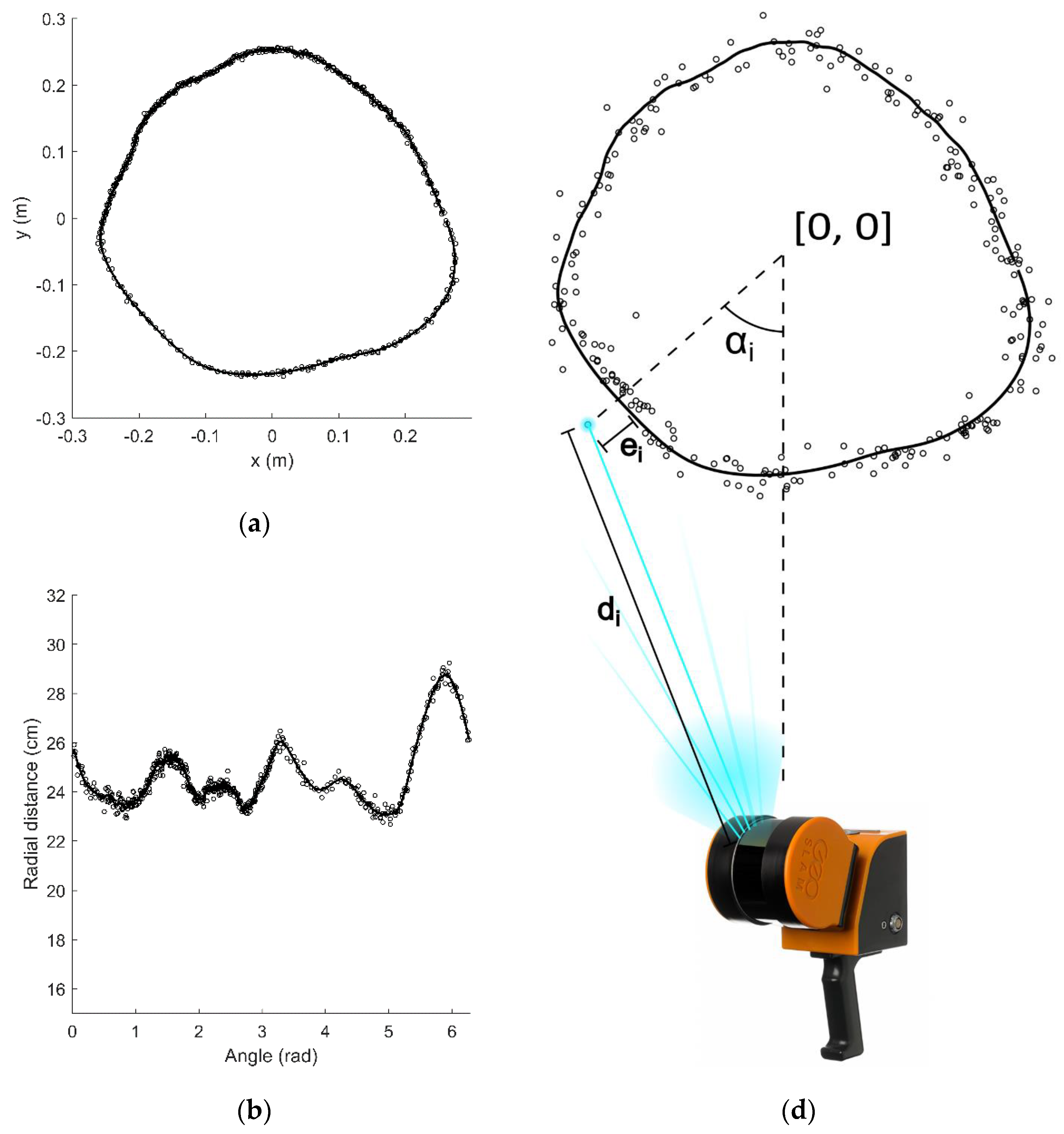
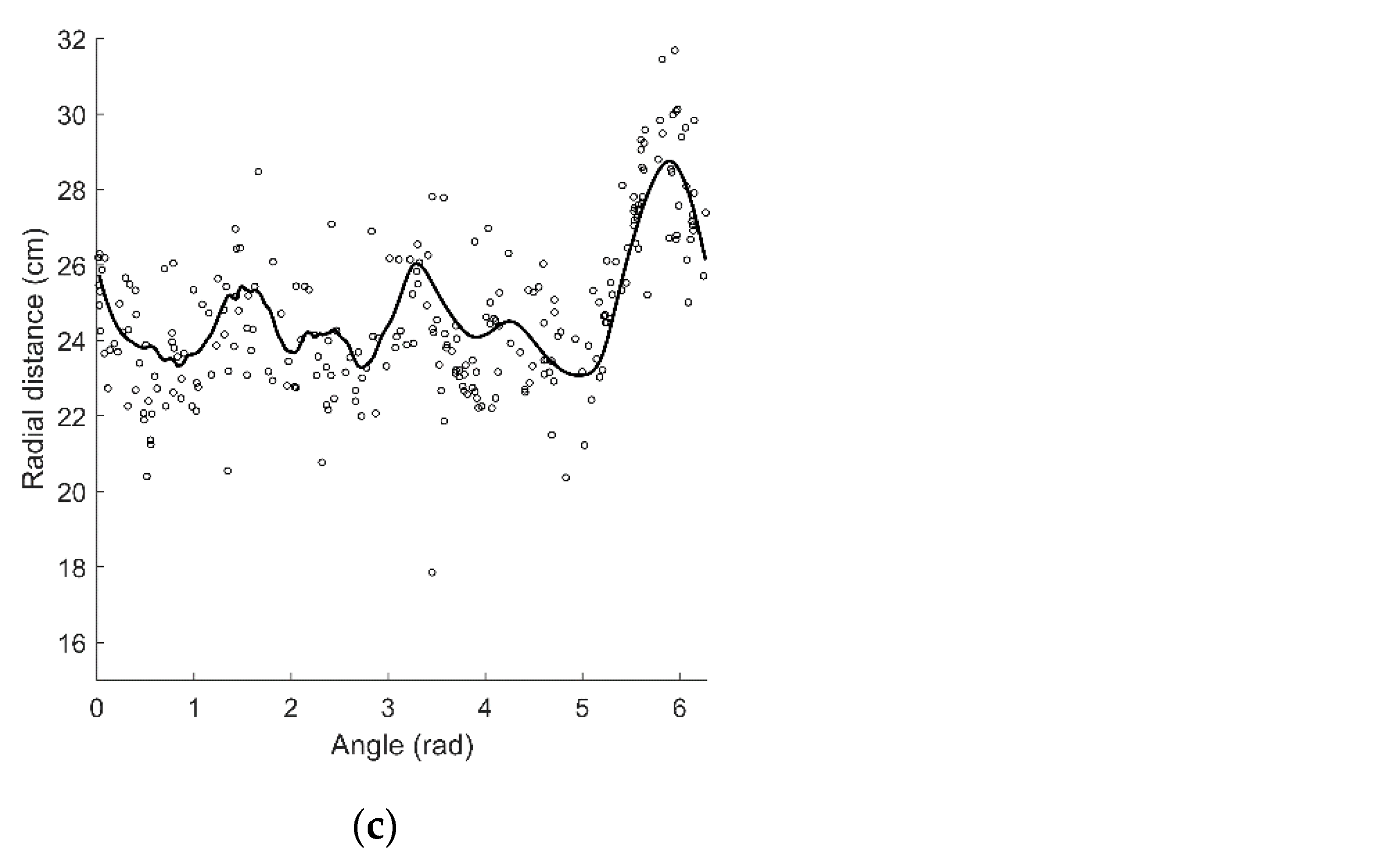
Figure 4.
The MLS trajectory segments are shown in different colors; the tree cross-section points in the MLS data are colorized according to the trajectory segments from which they were acquired.
Figure 4.
The MLS trajectory segments are shown in different colors; the tree cross-section points in the MLS data are colorized according to the trajectory segments from which they were acquired.
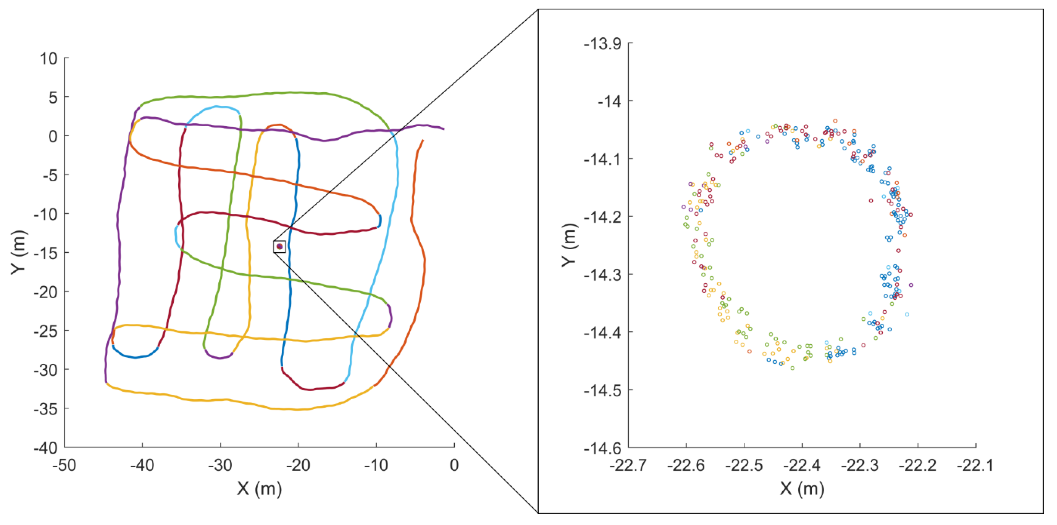
Figure 5.
The RANSAC parameters: tw—tolerance belt width; r—radius of the candidate circle fitted to the random subsample; rin and rout—inner and outer radius of the tolerance belt.
Figure 5.
The RANSAC parameters: tw—tolerance belt width; r—radius of the candidate circle fitted to the random subsample; rin and rout—inner and outer radius of the tolerance belt.
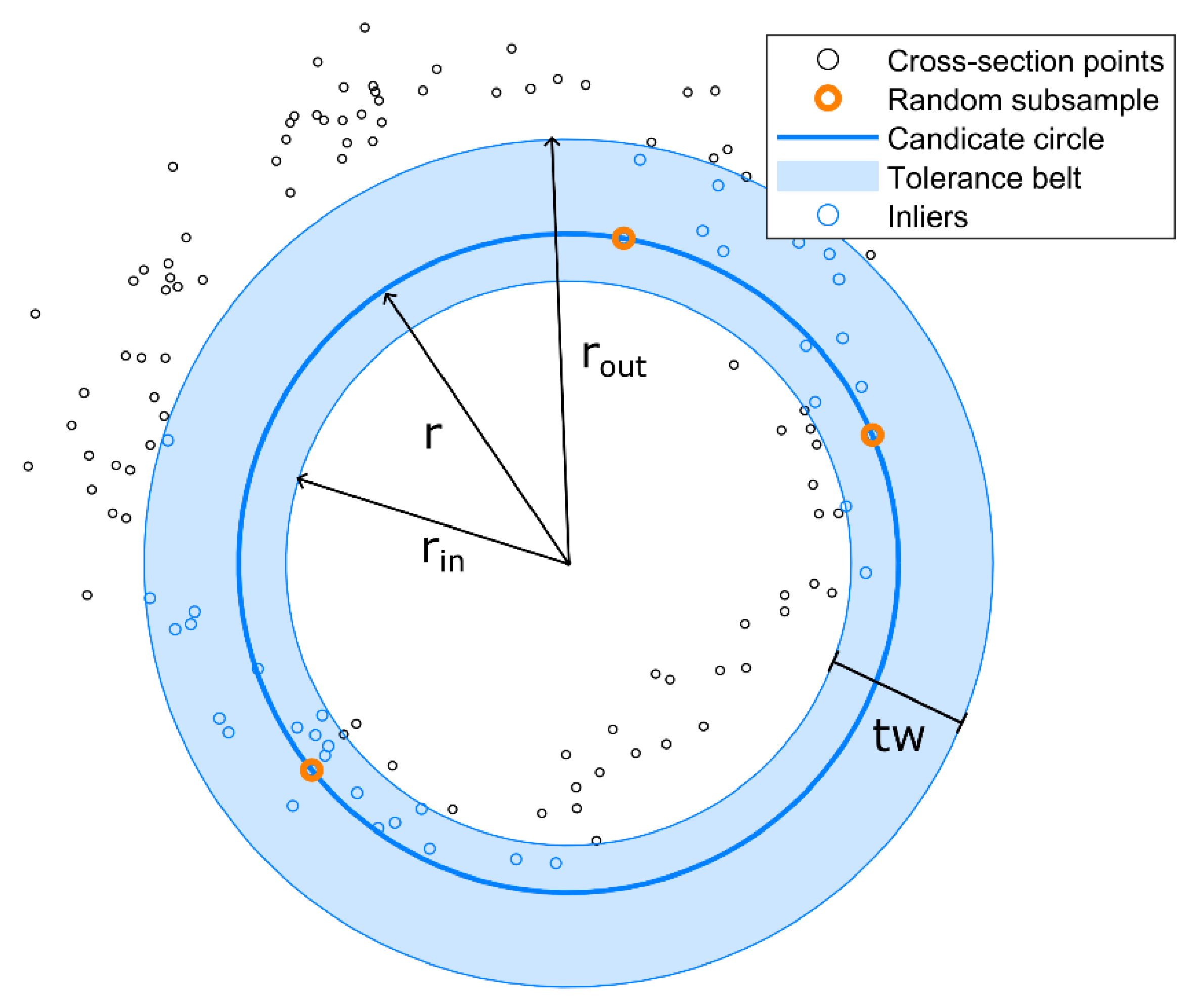
Figure 6.
Histograms of radial residuals for Norway spruce and European beech (a) and of mean radial residuals in cross-sections (b), including the PDFs of the fitted normal distributions for the two species (lines).
Figure 6.
Histograms of radial residuals for Norway spruce and European beech (a) and of mean radial residuals in cross-sections (b), including the PDFs of the fitted normal distributions for the two species (lines).
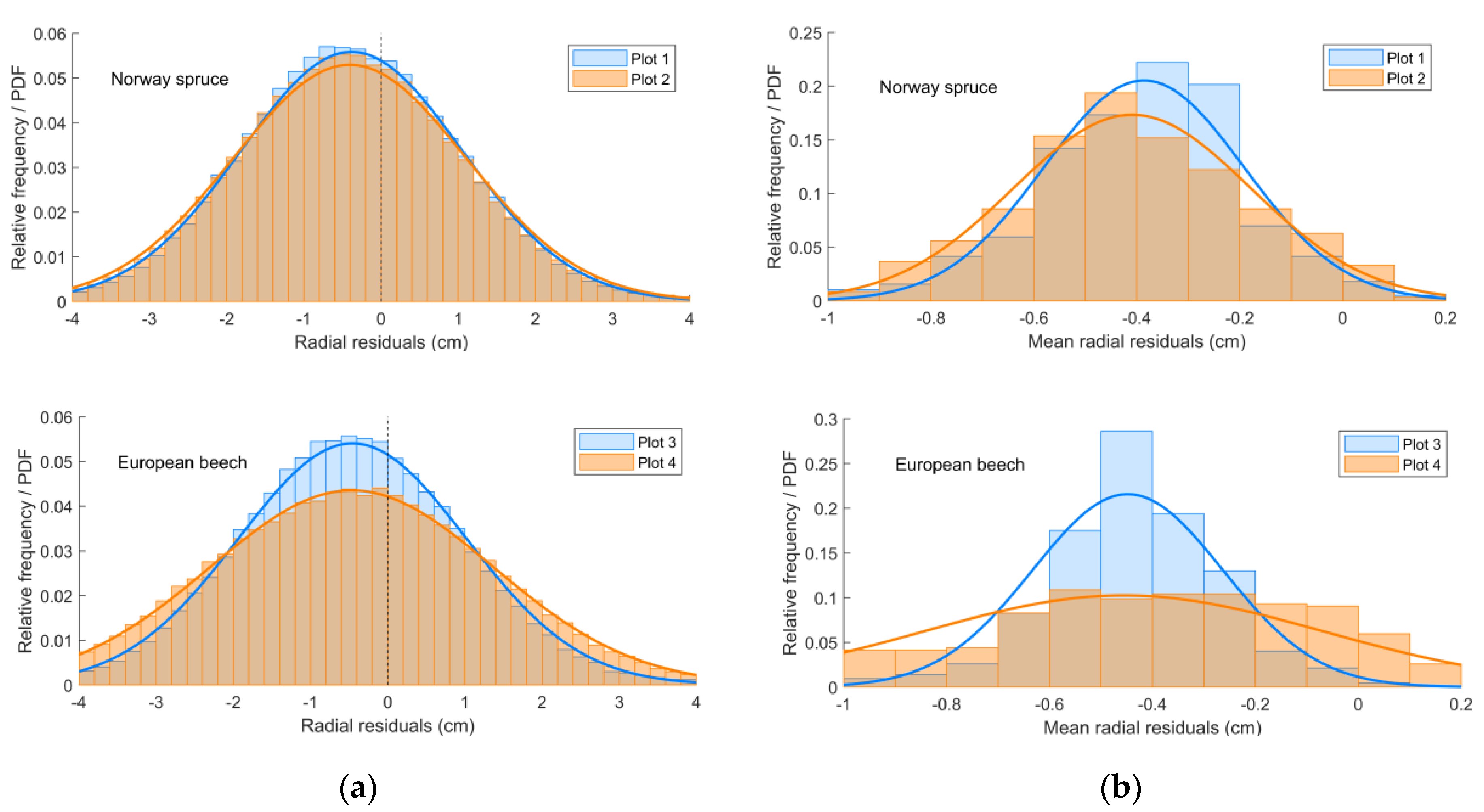
Figure 7.
Vertical distribution of mean (a) and standard deviation (b) of residuals in cross-sections.
Figure 7.
Vertical distribution of mean (a) and standard deviation (b) of residuals in cross-sections.
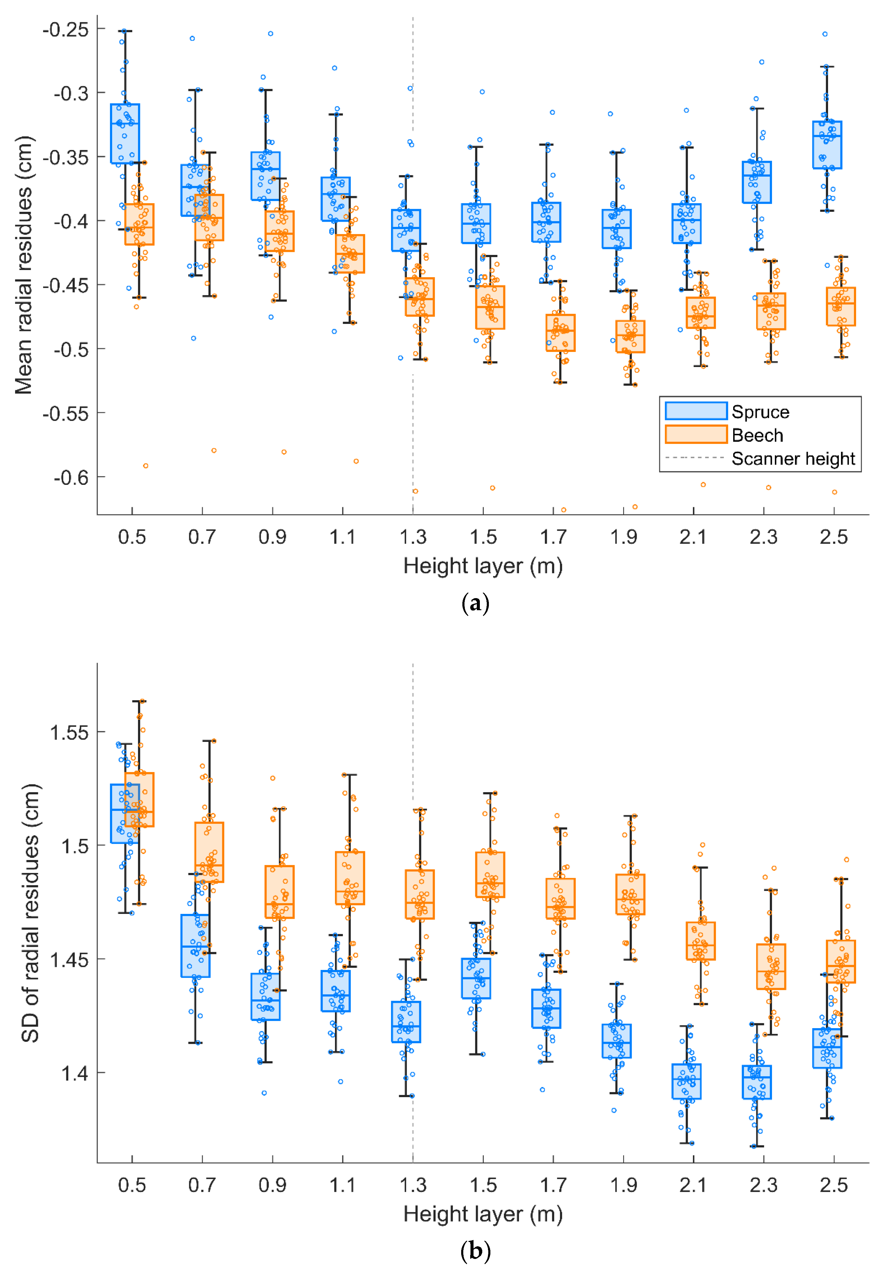
Figure 8.
The dependence of radial residuals on return distance. The returns are plotted along with the linear trends (solid) and their 95% prediction confidence intervals (dashed).
Figure 8.
The dependence of radial residuals on return distance. The returns are plotted along with the linear trends (solid) and their 95% prediction confidence intervals (dashed).
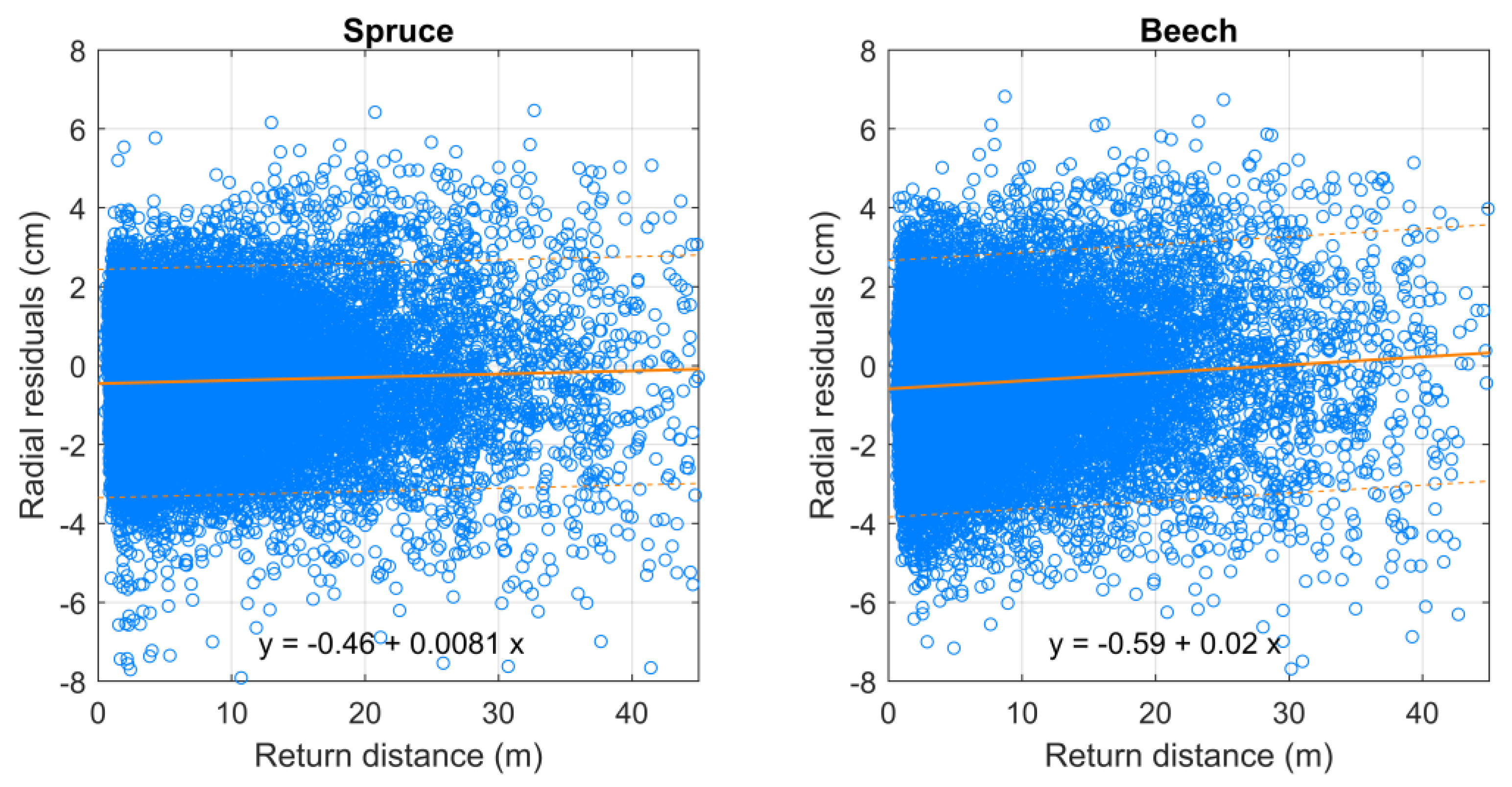
Figure 9.
The dependence of radial residuals on incidence angle. The returns are plotted along with the overall linear trends (solid orange lines) and their 95% prediction confidence intervals (dashed orange lines). The black lines show the detected trends for distance classes, as indicated in the legend.

Figure 10.
The errors of position and radius estimates for point structures acquired from individual scan lines (left) and from the simulated point structures (right).
Figure 10.
The errors of position and radius estimates for point structures acquired from individual scan lines (left) and from the simulated point structures (right).
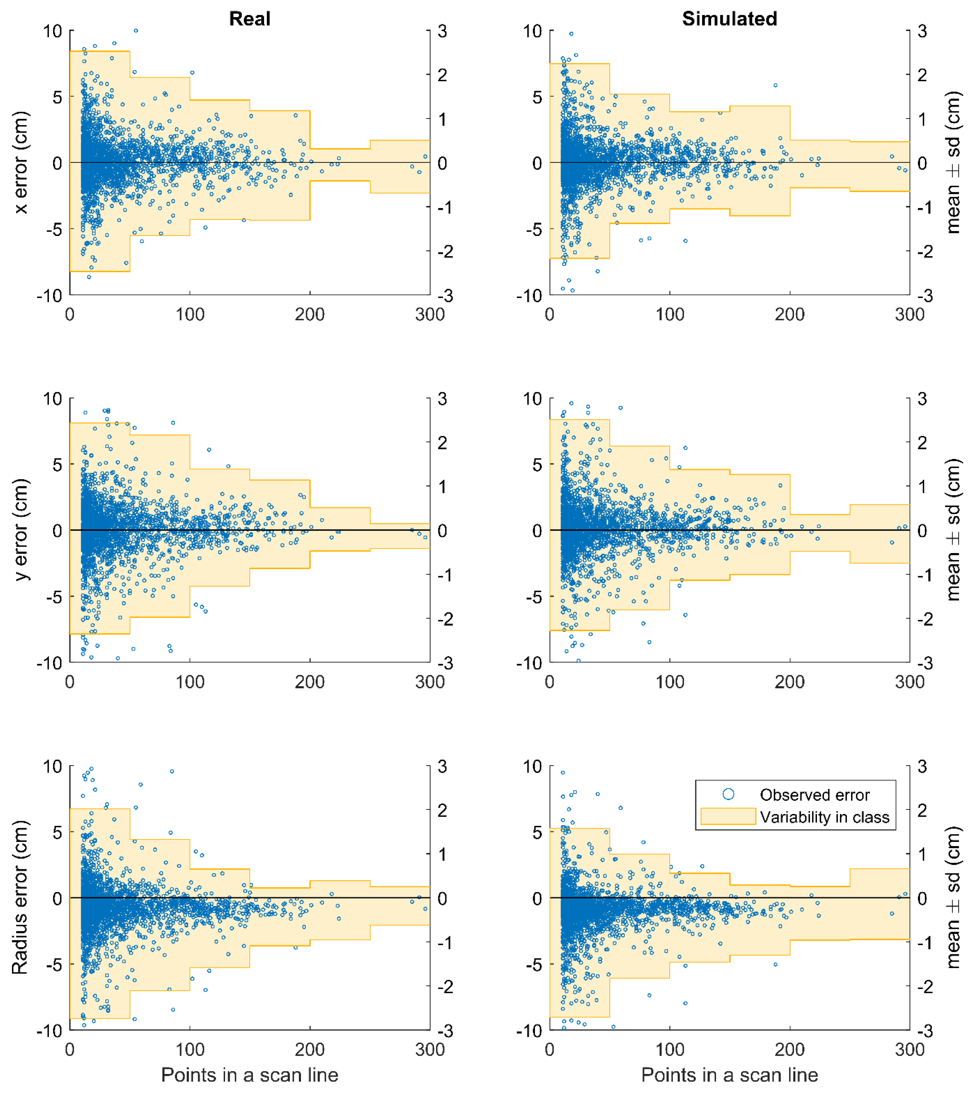
Figure 11.
The estimated cross-section radius bias (above) and radius RMSE (below) dependence on tolerance width and asymmetry, displayed as colormaps and contour plots. The bottom corners beyond the red dashed line represent the area where the asymmetry exceeds half of the tolerance width, i.e., the original subsample points are not included in inliers.

Table 1.
Characteristics of research plots.
| Species | Norway Spruce | European Beech | ||
|---|---|---|---|---|
| Plot | 1 | 2 | 3 | 4 |
| Tree count | 43 | 62 | 46 | 50 |
| DBH range (cm) | 32–64 | 21–62 | 32–56 | 33–66 |
| Mean DBH (cm) | 44 | 41 | 42 | 43 |
Table 2.
Normal distribution parameter estimates together with 95% confidence intervals for all residuals and mean residuals in cross-sections, according to the species.
Table 2.
Normal distribution parameter estimates together with 95% confidence intervals for all residuals and mean residuals in cross-sections, according to the species.
| Species | Plot | Residuals | Mean Residuals in Cross-Sections | ||
|---|---|---|---|---|---|
| Mean | SD | Mean | SD | ||
| Spruce | 1 | −0.38 (−0.39, −0.37) | 1.43 (1.42,1.44) | −0.39 (−0.41, −0.37) | 0.19 (0.18, 0.20) |
| 2 | −0.40 (−0.41, −040) | 1.51 (1.50, 1.51) | −0.41 (−0.43, −0.39) | 0.23 (0.22, 0.24) | |
| Beech | 3 | −0.46 (−0.47, −0.45) | 1.48 (1.47, 1.48) | −0.45 (−0.47, −0.43) | 0.18 (0.17, 0.20) |
| 4 | −0.43 (−0.44, −0.42) | 1.85 (1.84, 1.86) | −0.46 (−0.49, −0.42) | 0.38 (0.36, 0.31) | |
Disclaimer/Publisher’s Note: The statements, opinions and data contained in all publications are solely those of the individual author(s) and contributor(s) and not of MDPI and/or the editor(s). MDPI and/or the editor(s) disclaim responsibility for any injury to people or property resulting from any ideas, methods, instructions or products referred to in the content. |
© 2024 by the authors. Licensee MDPI, Basel, Switzerland. This article is an open access article distributed under the terms and conditions of the Creative Commons Attribution (CC BY) license (https://creativecommons.org/licenses/by/4.0/).
Share and Cite
MDPI and ACS Style
Kuželka, K.; Surový, P. Noise Analysis for Unbiased Tree Diameter Estimation from Personal Laser Scanning Data. Remote Sens. 2024, 16, 1261. https://doi.org/10.3390/rs16071261
AMA Style
Kuželka K, Surový P. Noise Analysis for Unbiased Tree Diameter Estimation from Personal Laser Scanning Data. Remote Sensing. 2024; 16(7):1261. https://doi.org/10.3390/rs16071261
Chicago/Turabian StyleKuželka, Karel, and Peter Surový. 2024. "Noise Analysis for Unbiased Tree Diameter Estimation from Personal Laser Scanning Data" Remote Sensing 16, no. 7: 1261. https://doi.org/10.3390/rs16071261
Note that from the first issue of 2016, this journal uses article numbers instead of page numbers. See further details here.