Article

Raster Scale Farmland Productivity Assessment with Multi-Source Data Fusion—A Case of Typical Black Soil Region in Northeast China

1
Key Laboratory of Sustainable Forest Ecosystem Management-Ministry of Education, Northeast Forestry University, Harbin 150040, China
2
School of Forestry, Northeast Forestry University, Harbin 150040, China
3
Research and Development Center of Big Data for Ecosystem, Northeast Forestry University, Harbin 150040, China
*
Author to whom correspondence should be addressed.
Remote Sens. 2024, 16(8), 1435; https://doi.org/10.3390/rs16081435
Submission received: 20 February 2024 / Revised: 6 April 2024 / Accepted: 16 April 2024 / Published: 18 April 2024

Abstract

:
Degradation of black soil areas is a serious threat to national food security and ecological safety; nevertheless, the current lack of information on the location, size, and condition of black soil farmland productivity is a major obstacle to the development of strategies for the sustainable utilization of black soil resources. We synthesized remote sensing data and geospatial thematic data to construct a farmland productivity assessment indicator system to assess the productivity of black soil cropland at the regional scale. Furthermore, we conducted research on the spatial differentiation patterns and a spatial autocorrelation analysis of the assessment results. We found that farmland productivity within this region exhibited a decline pattern from south to north, with superior productivity in the east as opposed to the west, and the distribution follows a “spindle-shaped” pattern. Notably, the Songnen and Sanjiang typical black soil subregions centrally hosted about 46.17% of high-quality farmland and 53.51% of medium-quality farmland, while the Mondong typical black soil subregion in the west predominantly consisted of relatively low-quality farmland productivity. Additionally, farmland productivity displayed a significant positive spatial correlation and spatial clustering, with more pronounced fluctuations in the northeast–southwest direction. The developed indicator system for farmland productivity can illustrate the spatial differentiation and thereby offer a valuable reference for the sustainable management of farmland resources.

1. Introduction

Farmland is closely linked to food security, ecological sustainability, and human development, serving as an indispensable resource and material foundation for humanity [1,2]. In the current era of extensive land degradation, food security and sustainable agricultural development challenges are substantial. Factors such as climate change, population growth, economic development, and land-use alterations continually intensify the strain on farmland resources [3,4]. There is a consensus that the most critical aspect of land degradation lies in reducing land productivity attributed to natural factors or human activities [5,6,7,8]. In response to land degradation’s status as a significant environmental threat, the United Nations Sustainable Development Solutions Network (SDSN) recommends quantifying the pivotal role of farmland productivity in achieving the United Nations Sustainable Development Goals (SDGs), particularly SDG 2 (Zero Hunger) and SDG 15.3 (Land Degradation Neutrality), to address the food security crisis [9,10,11]. Therefore, an immediate requirement exists to develop a set of reasonably efficient and reproducible large-scale farmland productivity assessment methodologies for global land degradation mapping [12]. This is essential to facilitate necessary actions in regions experiencing severe land degradation, with the goal of ensuring human well-being and food security.
Farmland productivity assessment should prioritize farmland productivity and systematically elucidate its fundamental structure, connotations, and dimensions [13,14]. Recently, theories and methodologies related to farmland productivity assessment have become more sophisticated, and the multifunctionality of farmland has been acknowledged [15,16]. Assessment criteria have shifted from singular natural elements such as soil, climate, and topography towards a comprehensive approach that encompasses multi-level indicators spanning ecological, socio-economic, and human activity domains [17,18,19]. Bünemann et al. systematically synthesized international soil quality definitions, assessment methodologies, and indicator selection, proposing that soil quality assessment should encompass the identification of soil threats, functions, and ecosystem services [20]. Wu et al. asserted that cultivated productivity, site conditions, and soil health collectively determine the sustainable development potential of farmland, emphasizing the need to fully consider the coupling and coordination effects among these three subsystems [21]. Shi et al. established a regional farmland quality assessment system grounded in a resource–asset–capital attribute analysis framework, which, in addition to its focus on natural factors, incorporates socio-economic elements such as transportation, location, and investments in agricultural technology [22]. These studies offer a comprehensive and detailed perspective for an integrated assessment of farmland productivity. Nevertheless, the heavy reliance on field observations has resulted in a significant field survey workload, leading most studies to concentrate on a small scale, with certain limitations in assessing farmland productivity on a broader scale.
Remote sensing is a potent monitoring tool for the assessment of farmland productivity and has witnessed widespread utilization in large-scale assessments in recent decades [23,24,25,26]. Liu et al. employed the global agro-ecological zone (GAEZ) model to calculate the dataset concerning potential crop yield in China, thus unveiling the influence of urban expansion on potential yields from 1990 to 2010 [27]. Prăvălie et al. utilized geospatial data to assess the extent and occurrence of five relevant land degradation processes in arable land across the globe [28]. Sciortino et al. utilized medium- and high-resolution remote sensing data to monitor land productivity status and trends at national and local levels [29]. Montfort et al. analyzed potential factors affecting vegetation productivity to assess land degradation trends in less developed regions, such as Mozambique [30]. Dameneh et al. carried out a long time-series analysis of land desertification trends, combining vegetation and climate indices to identify regions susceptible to land degradation and to formulate a prioritized work program [31]. However, current research lacks the assessment of black soil that guarantees food security, and we synthesize Landsat remote sensing data and geospatial thematic data such as climate and topography to assess the farmland productivity of black soil at the regional scale, in terms of the synchronicity and holism considerations of the indicator system.
The suitability of farmland productivity assessment methods is closely related to spatial location. Targeting different assessment objects or adopting distinct assessment methodologies exerts a significant impact on assessment outcomes [12,32]. Black soil, characterized by humus-rich surface layers and fertile soil, is globally acknowledged as a scarce, high-productivity, and degradation-prone premium land type. In recent years, it has garnered extensive attention and research from scholars worldwide [33,34]. Among the world’s four largest black soil regions, the black soil region of northeast China has historically remained devoid of erosion prevention or soil conservation initiatives. High agricultural production inputs, advanced technological conditions, and the use of pesticides and chemical fertilizers have increased crop yields. However, this conceals the fundamental decline in black soil farmland productivity, which poses a threat to national food security and ecological safety [35,36]. Therefore, assessing farmland productivity in the black soil region of northeast China is pivotal for ensuring food security and promoting the sustainable utilization of farmland resources.
The primary objective of this study is to synthesize remote sensing and geothematic data to carry out a farmland productivity assessment of the typical black soil region of northeast China at the raster scale through remote sensing. Our specific aims include the following: (1) To develop a universally applicable indicator system for farmland productivity assessment; (2) To elucidate the spatial differentiation pattern of farmland productivity in the typical black soil region of northeast China; (3) To reveal the spatial correlation of farmland productivity in the typical black soil region of northeast China. This study’s findings will provide valuable insights for decision-makers in the realm of sustainable farmland utilization and the enhancement of regional farmland productivity to ensure food security.

2. Materials and Methods
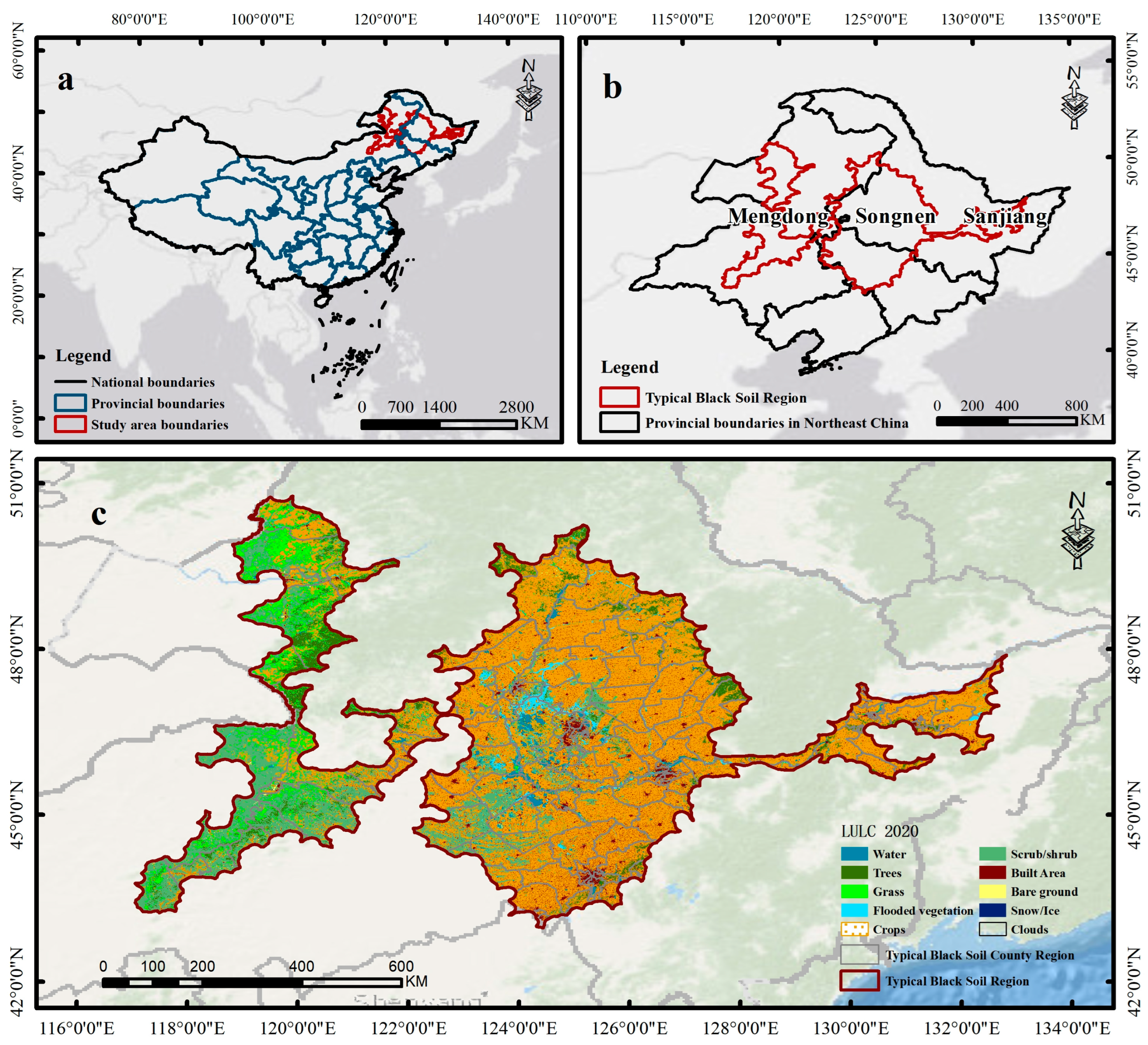
2.1. Study Area

The black soils referred to in this study correspond to Mollisol in the U.S. Soil System Classification and Isohumosol in the Chinese Soil System Classification. The Northeast Typical Black Soil Region (NETBSR) is the most significant crop-yielding region in China (Figure 1). It is situated between 116°E–136°E and 42°N–52°N, covering an expansive area of 333,000 km2. The area of black soil and chernozem in the area is 59.7 and 98.6 thousand km2, respectively, accounting for 47.5% of the total area of the typical black soil area; the proportion of meadow soil in the interspersed area is 28.8%. Within this region, farmland comprises approximately 55.65% of the total NETBSR area, encompassing Heilongjiang Province (57.14% farmland), Jilin Province (25.47%), the Inner Mongolia Autonomous Region (17.32%), and Liaoning Province (0.07%). NETBSR spans four provincial-level administrative divisions, 21 municipal-level administrative divisions, and 138 county-level administrative divisions [37]. The NETBSR can be divided into three distinct typical black soil subregions (TBSSs) based on geographic location: Mengdong TBSS in the west, Songnen TBSS in the center, and Sanjiang TBSS in the east. The region experiences a temperate continental monsoon climate characterized by concurrent rainfall and warmth during the growing season. However, in the non-growing season, the soil undergoes deep freezing and remains frozen for an extended period, with a noticeable seasonal frozen layer. The combined area of black soil and black calcareous soil within the district accounts for 47.5% of NETBSR’s total area. Additionally, there is an interspersed area of meadow soil, constituting 28.8%. Due to the absence of adequate soil and water conservation measures over the past century, soil erosion in the black soil layer has escalated recently, leading to a decline in black soil farmland productivity. This situation poses a significant challenge to the sustainable utilization of China’s black soil resources and food security.

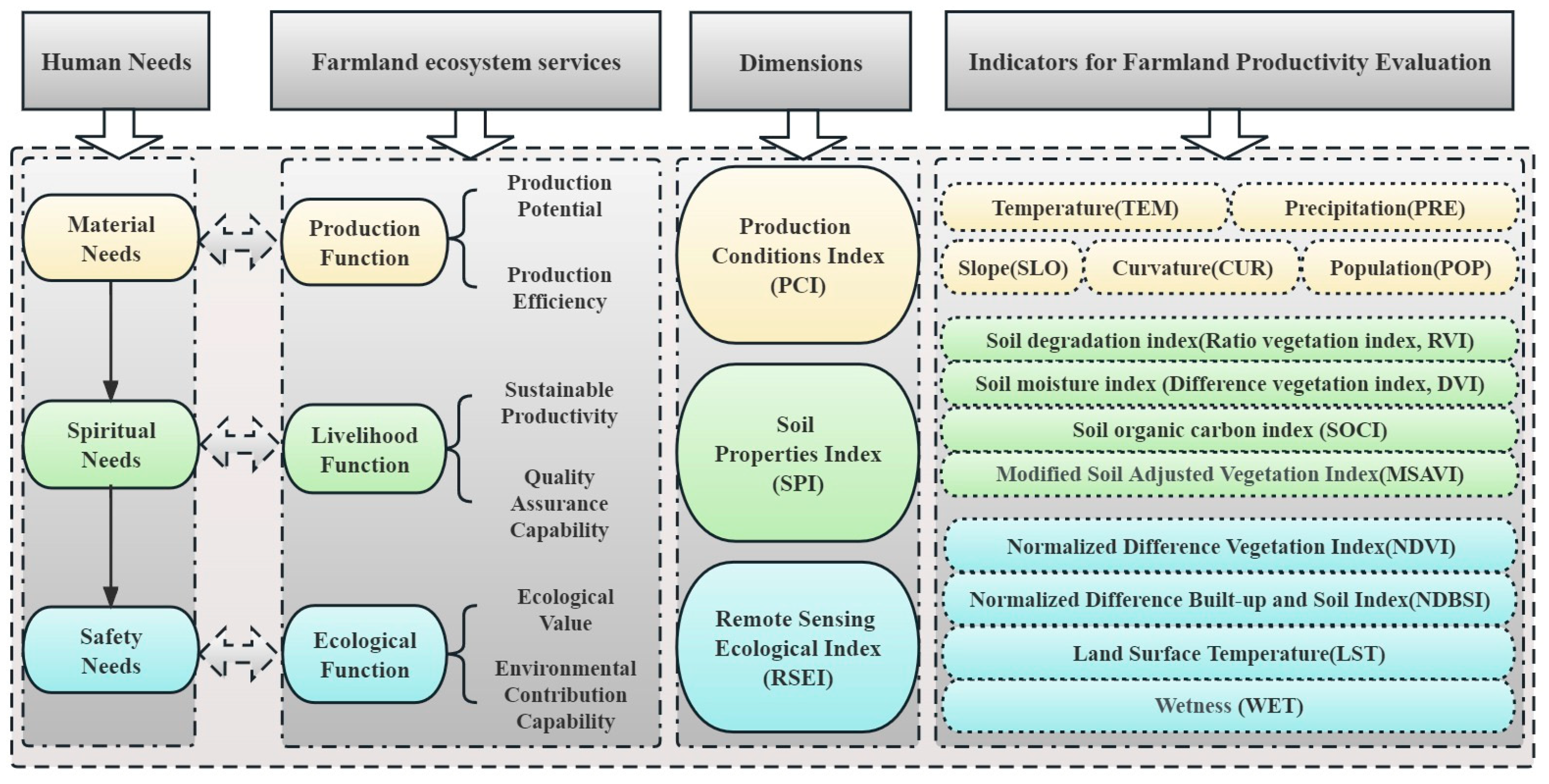
2.2. Chosen Indicators for the Farmland Productivity Assessment System

Defining the connotation of farmland productivity is the cornerstone of farmland productivity assessment, serving as a fundamental theoretical underpinning for farmland productivity research, land preservation, and remediation [14,38]. Diverse regional demands for farmland resources have led to the emergence of varying perspectives and assessment methodologies in farmland assessment systems, resulting in the absence of a universally accepted definition of “farmland productivity” [39,40]. Farmland productivity requirements differ among various stakeholders. The Chinese government, committed to farmland protection and sustainable land resource management, emphasizes the preservation of farmland. Local governments, prioritizing regional economic development, sometimes view farmland preservation as hindering progress and advocate for non-farmland use. Farmers focus on the economic output potential of farmland and seek social security for farmland. Urban residents are concerned with the environmental productivity of farmland and aspire to reconnect with idyllic life, thereby placing ecological, aesthetic, and cultural demands on farmland [41,42]. Hence, drawing upon the Ecosystem Services Cascade (ESC) framework [43], this study comprehensively considers human needs, whether direct or indirect, arising from the functions provided by farmland ecosystems [44,45,46]. This comprehensive perspective defines the connotation of farmland productivity as follows: The extent or capacity of farmland to fulfill human material, spiritual, and safety needs in terms of production, livelihood, and ecology through a multitude of interactions and system linkages within the farmland ecosystem. On this foundation, we have formulated a three-dimensional assessment indicator system (Figure 2), encompassing the Production Conditions Index (PCI), Soil Properties Index (SPI), and Remote Sensing Ecological Index (RSEI). The relationships are described below:
Fulfilling human material needs mirrors the productive role of farmland ecosystems. The most basic and stable function of farmland ecosystems is to enable agricultural production and income generation, which is essentially centered on the potential and efficiency of farmland production as determined by production conditions dominated by natural elements [43,47]. Population reflects the potential impact of human activities, particularly unsustainable farming practices, on the farmland productivity. In densely populated areas, urbanization and human disturbance are often more pronounced, and these factors may lead to greater pressure on farmland [48]. Therefore, in the context of the PCI, human material needs can be delineated in terms of climatic conditions, such as temperature (TEM) and precipitation (PRE), along with topographic conditions, including slope (SLO) and curvature (CUR), which constitute the natural factors. Additionally, human activities, as represented by the population (POP), are a vital component of this assessment.
Meeting human spiritual needs reflects the livelihood function of farmland ecosystems. With the advancement of productivity, human priorities have transitioned from merely increasing the quantity of agricultural products to an emphasis on achieving high product quality, necessitating farmland to exhibit both high sustainable productivity and a robust capacity for ensuring product quality. The level of farmland productivity, in turn, profoundly influences human economic development and quality of life. Soil properties stand out as pivotal factors in assuring agricultural production sustainability and product quality stability [3,49]. Hence, in the context of the SPI, catering to the spiritual needs of individuals within farmland ecosystems involves using surrogate indicators, such as the Soil Degradation Index (Ratio Vegetation Index, RVI), Soil Moisture Index (Difference Vegetation Index, DVI), Soil Organic Carbon Index (SOCI), and Modified Soil Adjusted Vegetation Index (MSAVI).
Addressing human safety needs underscores the ecological role of farmland ecosystems. With the progression of urbanization, there is an increasing emphasis on the eco-environmental contributions of farmland ecosystems. On one hand, the ecological quality of farmland profoundly impacts the level of sustainable farmland use and the quality of agricultural products. On the other hand, it reflects the ecological value inherent to farmland itself, a dimension of growing significance within the context of ecological civilization construction [50]. Therefore, utilizing the RSEI, which is an ecological environment quality assessment system, in conjunction with critical indicators, such as the Greenness Index (Normalized Difference Vegetation Index, NDVI), Dryness Index (Normalized Difference Built-Up and Soil Index, NDBSI), Heat Index (Land Surface Temperature, LST), and Humidity Index (Wetness, WET), all directly associated with the quality of the ecological environment, allows for an intuitive and swift evaluation of ecological security status [51].

2.3. Sources and Pre-Processing of Indicator Data

We derived the five indicators’ data in the PCI from analyzing fundamental geospatial data. Climatic data (1 km × 1 km) for TEM and PRE were extracted from the spatially interpolated dataset representing average meteorological conditions in China. SLO and CUR were determined through spatial analysis of digital elevation data (30 m × 30 m) from ASTER GDEM V3. The data of POP were sourced from LandScan Global (1 km × 1 km), a global population distribution database developed by the US Department of Energy’s Oak Ridge National Laboratory.
Data for the eight indicators in the two dimensions of SPI and RSEI were acquired by extracting bands from remotely sensed images and conducting the corresponding band operations. Remote sensing image data (30 m × 30 m) were sourced from Landsat 8–9 OLI/TIRS Collection 2 Level-2 high-resolution imagery provided by the United States Geological Survey (USGS) through their website (https://earthexplorer.usgs.gov/ (accessed on 2 September 2022)). Selection of remote sensing images with less than 5% cloud cover was ensured. To ensure the validity of the assessment results, we optimized the time for the period from July to September, when the vegetation on the farmland is in full growth. This data product encompasses surface reflectance in multispectral bands and incorporates a surface temperature product in the thermal infrared band (TIRS Band 10). It adheres to the conventional Landsat Ecosystem Disturbance Adaptive Processing System (LEDAPS) procedure, encompassing atmospheric corrections, geometric corrections, and radiometric calibrations.
All data acquisition occurred in the year 2020. Following the collection or calculation of all indicators (Table 1), each of the 13 indicators underwent processing, including projection raster, resampling, and outlier removal, ultimately yielding raster maps for each indicator.
Except for SOCI, the other indicators listed in Table 1 are commonly used indicators that have been widely verified and applied, and their accuracy has been confirmed in several studies. Although the calculation of SOCI is based on empirical relationships of historical measurement data, these coefficients still provide us with relatively reasonable approximations in remote sensing band calculations in the absence of region-specific data, thus supporting our assessment of farmland productivity at the current geographic scale.

2.4. Farmland Productivity Assessment Model

To mitigate the influence on assessment results caused by variations in the base unit of the indicators during the calculation process, it is essential to standardize the indicators, making them dimensionless and homogenized. Given the attributes of the indicators, they were categorized into positive indicators (benefit-based indicators) and negative indicators (cost-based indicators), and the original values of each indicator were normalized (Equations (1) and (2)), ensuring a standardized range between [0, 1]. Mean centering (Equation (3)) aligned the PCA’s first principal component with the direction of maximum variance while eliminating discrepancies in variable means.
B I i = ( b i b m i n ) / ( b m a x b m i n )
B I i = ( b m a x b i ) / ( b m a x b m i n )
X = X μ
where B I i is the normalized pixel value of a certain indicator, b i is the pixel value of a certain indicator, and   b m a x , b m i n are the maximum and minimum values of the indicator, respectively. X is the original pixel value, and μ is the mean value.
The mean-centered and normalized data underwent principal component analysis (PCA) to derive indicator weights, which were subsequently integrated into a Linear Weighting Model (LWM) to compute the Farmland Productivity Composite Index (FPCI) through the following steps [55,56]:
(i) Conducting the Kaiser–Meyer–Olkin (KMO) test and Bartlett’s test to assess the suitability of the PCA model. (ii) Calculating the eigenvalues of the correlation matrix and the variance contribution ratio of each indicator, and determining the number of principal components K with the criterion that the eigenvalue is greater than 1 and the cumulative variance contribution ratio is greater than 80% [57]. (iii) Deriving linear combination coefficients using the factor loading values of the indicator correlation matrix (Equation (4)). (iv) Computation of the coefficients in the comprehensive score model based on the acquired linear combination coefficients (Equation (5)). (v) Calculation of the weights of each indicator by determining the ratio of the coefficients in the comprehensive score model (Equation (6)). (vi) Utilizing LWM to evaluate FPCI, which is expressed as the weighted sum of the indicator values and their corresponding weights for each assessment unit after identifying the principal components (Equation (7)). The primary calculation formula is as follows:
θ i = α i / A k
λ i = e i X i / X i
F i = λ i / λ
F P C I = i = 1 n e i F i
where θ i is the linear combination coefficients for the i indicator; α i is the factor loading values for the i indicator; A is the eigenroot for the K principal components; λ i is the coefficients in the comprehensive score model for the i indicator; e i is the indicator value for the i indicator; X i is the principal component variance; F i is the weight for the i indicator; and n is the number of assessment units.
The computed FPCI value’s magnitude served as a surrogate for the farmland productivity level. Based on previous criteria for classifying farmland productivity categories, the FPCI was stratified into ten grades utilizing the equal spacing approach. Subsequently, grades 1–3 were designated as high-quality farmland, grades 4–7 as medium-quality farmland, and grades 8–10 as low-quality farmland [14,55].

2.5. Spatial Analysis of Farmland Productivity

Spatial autocorrelation analysis was employed to investigate the spatial correlation characteristics of farmland productivity. Global Moran’s I (Equation (8)) was utilized to gauge the extent of spatial clustering or differentiation of attribute values, which falls within the range of (−1, 1). When Moran’s I is positive, it signifies a spatial positive correlation, and a higher value suggests a more pronounced spatial correlation. The z-value was employed to denote data dispersion, with a threshold of 1.96 for the two-sided test and a 95% confidence interval of the normal distribution as the limit. A z-value greater than 1.96 indicates significant spatial positive autocorrelation, signifying non-significant differences between the observation point’s value and surroundings, indicating spatial clustering. Conversely, a z-value lower than −1.96 implies the opposite, and if the Z-value falls between −1.96 and 1.96, it signifies that the spatial autocorrelation of the study indicator is not significant and is randomly distributed across the study area. The p-value is used to indicate probability, which is convenient for hypothesis testing of spatial autocorrelation.
The G i * statistical index (Equation (9)) proposed by Getis and Ord, a local spatial autocorrelation indicator, was employed to identify cold and hotspots in the study area’s farmland productivity. This method aims to explore the spatial clustering of low or high values of farmland productivity, revealing areas where low or high values of farmland productivity tend to cluster. Hotspots refer to regions with a high concentration of attribute values, where the surrounding features also exhibit high values. Conversely, coldspots are the opposite, indicating areas with a clustering of low attribute values. Cold and hotspot analysis can only reveal the local spatial autocorrelation characteristics of farmland productivity, identifying clustered areas with similar productivity. It is unable to distinguish regions with significant differences in productivity within local space. However, Local Moran’s I and LISA values precisely address the shortcomings of the cold and hotspot analysis method.
Local Moran’s I (Equation (10)) classified the distribution of farmland productivity in the study area into five categories. When the value of Local Indicators of Spatial Association (LISA) is positive, it indicates a spatial cluster, including “High-High Cluster” (H-H) and “Low-Low Cluster” (L-L), signifying that the value of the observation point itself and the value of its surrounding observation points are both higher or lower. Conversely, a negative LISA value indicates a spatial outlier, including “Low-High Isolated” (L-H) and “High-Low Isolated” (H-L), which means that the value of the observation point itself is higher (or lower), while the values of the surrounding observation points are lower (or higher), reflecting the distribution of high and low neighbors. “Not Significant” (NS) denotes that the value of the observation point and the value of its surrounding observation points are not statistically significant.
G l o b a l   M o r a n s   I = n i = 1 n j = 1 n W i j Y i Y ¯ Y j Y ¯ i = 1 n j = 1 n W i j i = 1 n Y i Y ¯
G i * = j = 1 n W i j Y j j = 1 n Y j
L o c a l   M o r a n s   I = Y i Y ¯ i = 1 n Y i Y ¯ 2 n j = 1 n W i j Y i Y ¯
where n is the total number of spatial units; W i j is the spatial weight matrix; Y ¯ is the pixel mean; and Y j , Y i are the elemental attribute values of the spatial units.
The center of gravity and the trend of farmland productivity distribution in NETBSR are depicted using a standard deviation ellipse (SDE) [58]. The SDE primarily consists of three components: the rotation angle θ, the standard deviation along the major axis x, and the standard deviation along the minor axis y (Equations (11)–(13)). Its distribution range corresponds to the primary extent of spatial farmland productivity distribution; the rotation angle indicates the main trend direction of the distribution, and the standard deviation along the major axis reflects the degree of dispersion of farmland productivity in the direction of the primary trend. The orientation of the major axis represents the dominant spatial orientation of farmland productivity. A higher oblateness of the ellipse signifies a more directional farmland productivity distribution, while a more negligible difference in length between the major and minor axes indicates a less directional distribution.
x = i = 1 n X i X 2 n
y = i = 1 n Y i Y 2 n
tan θ = i = 1 n X i 2 i n Y i 2 + i = 1 n X i 2 i n Y i 2 + 4 i = 1 n X i Y i i 2 i = 1 n X i Y i
where X i , Y i are the spatial location coordinates of each data point; n is the total number of spatial units; and ( X , Y ) is the center of mass coordinates.

3. Results and Analysis

3.1. Construction of FPCI

The KMO coefficient was 0.836, and Bartlett’s test yielded a significance level of 0.000 (p < 0.001), indicating the rejection of the original hypothesis, implying a correlation between the indicators. The correlation matrix between the indicators revealed significant associations among the variables, with some correlation coefficients approaching 1. Consequently, this dataset was highly suitable for constructing the PCA-based indicator system of farmland productivity assessment. Analyzing the eigenvalues and cumulative variance contribution ratios (Table 2), four principal components with eigenvalues greater than one were extracted, accounting for 83.595% of the cumulative variance. It can be concluded that these four principal components, covering the majority of original variable information, can effectively substitute for the original variables.
The factor loading values in the indicator correlation matrix (Table 3) were obtained from the component matrix. The first principal component had significant loadings on SOCI, DVI, WET, NDBSI, NDVI, MSAVI, and RVI, representing the information contained in these seven variables. The second component had notable loadings on TEM, PRE, and LST, reflecting the information from these three variables. The third and fourth components exhibited higher loadings on SLO and POP, respectively, and the first and third components can jointly represent CUR. As noted above, it reiterated that the four principal components adequately represent the original 13 indicators.
After calculating the coefficients in the comprehensive score model using Equations (5) and (6), we obtained the weight values for the three-dimensional and the 13 assessment indicators developed in this study (Figure 3). It is evidenced that the weight values of the indicators were approximately equal, indicating that each indicator had a similar influence on the FPCI. Notably, SLO carried the most significant weight, accounting for 0.125 of the totals.

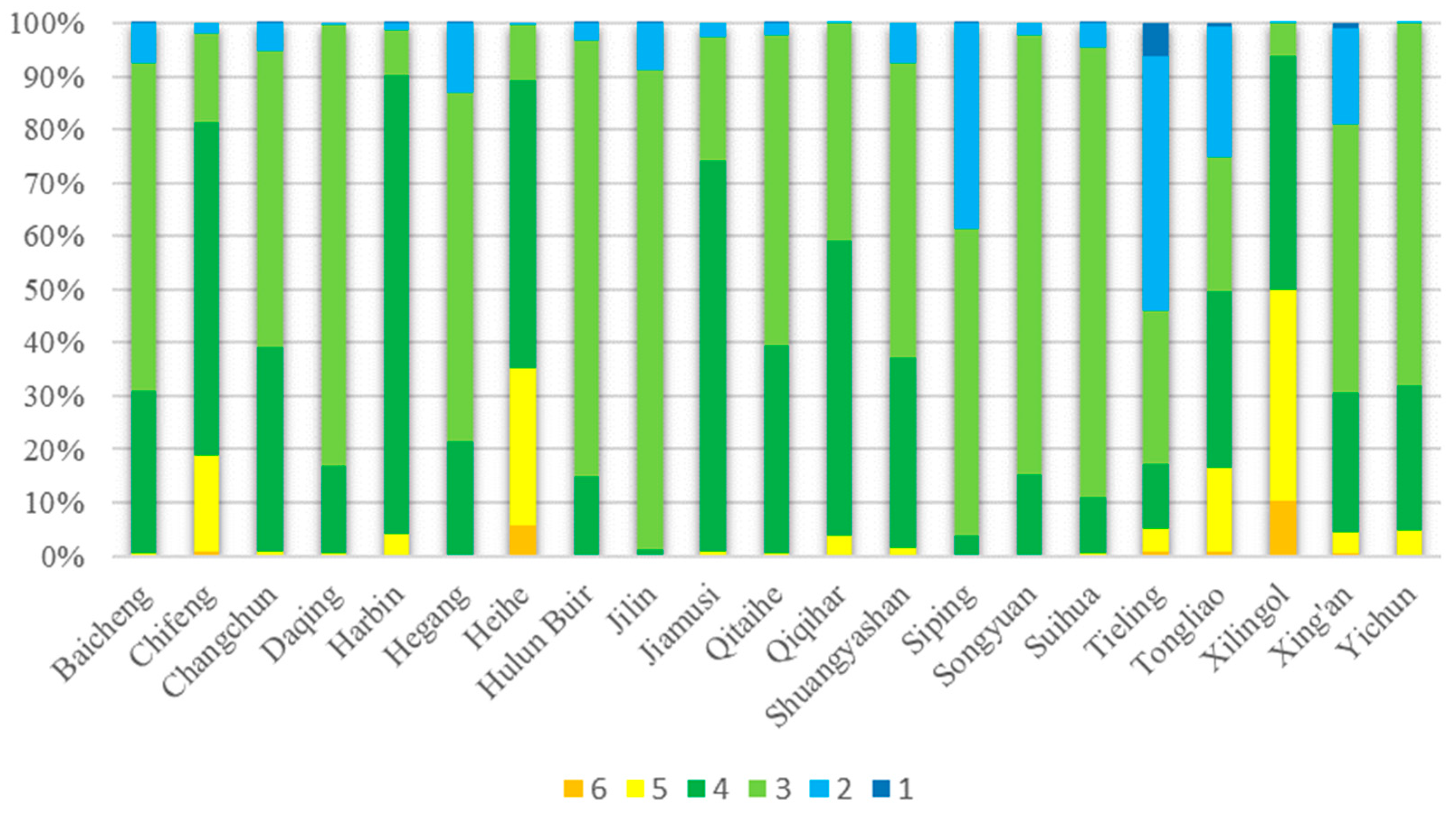
3.2. Spatial Distribution of FPCI at Various Scales

At the raster scale, this study utilized the equal spacing method to subdivide the FPCI of NETBSR within ten grades quantitatively. At the raster scale, grades 3–5 accounted for 88.72% of the entire NETBSR farmland area (Figure 4a), which suggested that FPCI levels were relatively similar within the NETBSR and were dominated by fairly medium to high levels. The total trend in the spatial distribution of FPCI in NETBSR was decreasing from south to north, with the east region being better than the west region (Figure 4b). A total of 46.17% of the high-quality farmland with FPCI grades 1–3 was mainly located in the south of the Songnen TBSS and the Sanjiang TBSS; 53.51% of the medium-quality farmland with FPCI grades 4–7 was primarily located in the north of the Songnen TBSS, and 0.32% of the low-quality farmland with FPCI grades 8–10 was mainly located in the west of the Mondong TBSS.
At the county scale (Figure 5), high FPCI grades were primarily found in several counties (districts) among the 138 county-level administrative districts located in NETBSR. These areas included Fujin, Longjiang, Wuchang, Baoqing, Shuangcheng, Bayan, and other districts and counties. Bin, Fuyu, Beilin, Wudalianchi, and other districts and counties had medium FPCI grades. In contrast, Chenbalhu Banner, Erguna City, Linxi County, and Uzhumqin Banner exhibited relatively low FPCI grades.
At the municipal scale, the FPCI of the 21 municipalities within the NETBSR displayed significant variations. Generally, it exhibited a “spindle-shaped” distribution with smaller values at the ends and higher values in the middle, with the majority of FPCI grades falling within the medium range, skewed toward higher values (Figure 6). Specifically, Heihe, Yichun, Jilin, Changchun, and Tieling cities were regions where higher FPCI grades were predominantly concentrated. In contrast, Hulunbeier and Tongliao cities and Xilin Gol league had relatively lower FPCI grades.

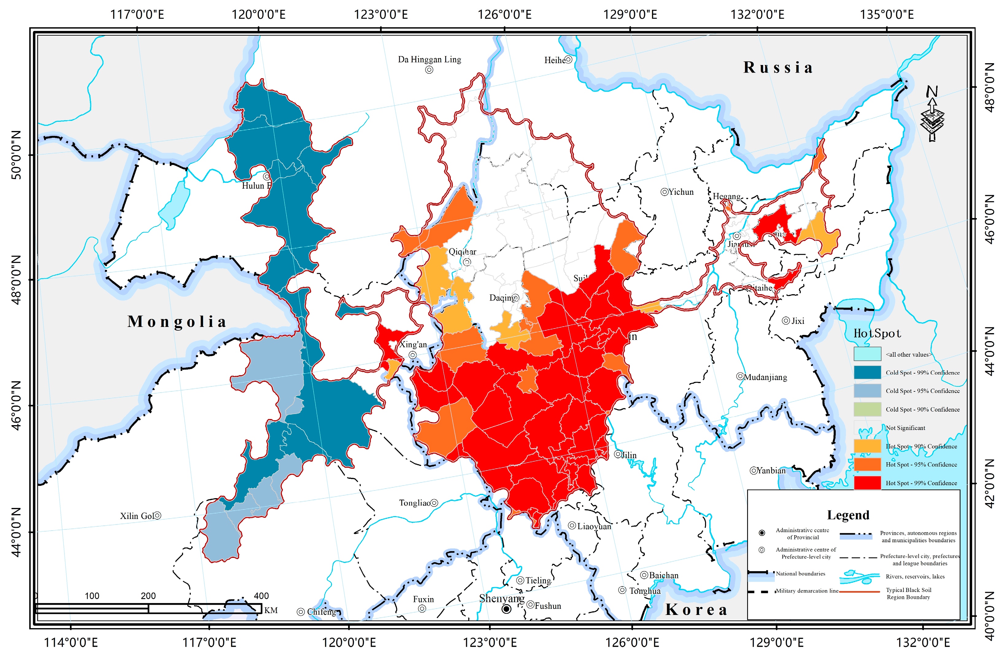
3.3. Spatial Correlation of FPCI at the Raster Scale

The results of the visualization of the cold–hotspot analysis of farmland productivity (Figure 7) revealed the pattern of its spatial distribution. This analysis identified clustered areas with similar productivity levels, hotspot areas (highly significant hotspot areas (99% confidence level), significant hotspot areas (95% confidence), and hotspot areas (90% confidence)) with a wide spatial distribution area, mainly distributed in the southern part of the Songnen TBSS in the center and part of the Sanjiang TBSS in the east, and coldspot areas (highly significant coldspot areas (99% confidence), significant coldspot areas (95% confidence), and coldspot region (90% confidence)) are mainly distributed Mengdong TBSS in the west. The distribution space of the FPCI hotspot region of NETBSR is basically the same as that of the raster high-value region of FPCI, and the distribution space of the coldspot region is basically the same as that of the raster low-value region. The distribution of hotspot and coldspot areas are concentrated.
The global Moran’s I of FPCI for NETBSR was 0.819 with a Z-value of 13.311, which passed the significance test (p = 0.001). This result indicated a highly significant positive spatial correlation and strong spatial clustering of the FPCI. Concerning the local spatial autocorrelation LISA aggregation map and spatial trend distribution plot (Figure 8), the FPCI was primarily composed of three categories within the study area: “H-H” (27.6%), “L-L” (20.1%), and “Not Significant” (NS) (46.8%). While “H-L” (1.6%) and “L-H” (3.9%) categories represented a smaller proportion, “H-H” was mainly distributed in the southern part of Songnen TBSS and parts of Sanjiang TBSS. At the same time, “L-L” was predominantly found in the eastern region of Mengdong TBSS, indicating significant spatial clustering of the FPCI in these two subregions.
A quantitative analysis of the directional trend of the FPCI center of gravity in NETBSR using the SDE revealed that an ellipse located at 125°E, 46°N, with approximately 541.86 km as the long semiaxis and 235.73 km as the short semiaxis, can encompass the area where about 68% of the FPCI in NETBSR was concentrated. The oblateness of the ellipse was 56.5%, and the length of the major axis was about 2.3 times that of the minor axis, indicating precise directional characteristics. The rotation angle was 86°, signifying that the FPCI center of gravity was more prominently distributed in the northeast–southwest direction than in the northwest–southeast direction, demonstrating distinct features.

3.4. Robustness of Results

We illustrate the reliability of the assessment results of farmland productivity in typical black soil regions by comparing and validating them with the dataset concerning potential crop yield in China by the global agro-ecological zone (GAEZ) model in both quantitative structure and spatial distribution [59].The dataset concerning potential crop yield in China by the GAEZ model was the result of a study conducted by Liu et al. [27], conducted to reveal the impact of urban expansion on farmland production potential, and we extracted annual standard crop yield data from the statistical yearbooks of Heilongjiang Province, Jilin Province, and the Inner Mongolia Autonomous Region.
In the crop production performance validation, we conducted regression analyses of annual standard crop yield data and our assessment results with the dataset concerning potential crop yield in China, respectively, to explore the correlation between the two assessment results and annual standard crop yields. In the spatial pattern correlation validation method, we compared the FPCI obtained in this study with the results of the dataset concerning potential crop yield in China by the GAEZ model for validation, both of which were evaluated from a multidimensional perspective of farmland productivity, and analyzed the spatial distribution pattern to explore the correlation between the two.
This study used the process of crop production performance validation, employing the FPCI of NETBSR as the independent variable (x) and the annual standard crop yield as the dependent variable (y) for linear regression analysis (Figure 9). Provided that the significance test (p < 0.001) and the test of multicollinearity (VIF < 5) were satisfied, although both have lower R2, the regression equation between FPCI and annual standard grain yield in this study had a higher degree of “best fit” (r = 0.637, R2 = 0.419) compared with the dataset concerning potential crop yield in China by the GAEZ model (r = 0.479, R2 = 0.230), indicating a stronger correlation between production FPCI and annual standard grain yield. which indicates a stronger correlation between production FPCI and annual standard grain yield.
We employed the spatial pattern correlation validation method to supplement the process of crop production performance validation. This involved comparing the farmland productivity assessment results obtained in this study with the existing GAEZ assessment results. The bivariate plot (Figure 10) illustrated that the spatial pattern distribution was notably consistent between the two datasets, with higher spatial correlation predominantly observed in the southern part of the study area compared to the northern part. Of the 138 counties included, 60.9% (84 counties) of the higher-middle spatial correlations were primarily located in the Mondong TBSS, the Sanjiang TBSS’s eastern section, and the Songnen TBSS’s southeastern portion. In contrast, the southwestern and northern portions of the Songnen TBSS displayed a lower spatial correlation.

4. Discussion

4.1. Rationalization of the Farmland Productivity Assessment System

Perceptions of the concepts, connotations, and dimensions of farmland productivity significantly influence the scientific precision and accuracy of farmland productivity assessment. Drawing upon the Ecosystem Services Cascade (ESC) framework [43], this study comprehensively integrates the human well-being aspects directly or indirectly derived from farmland ecosystems. Human material, spiritual, and safety needs correspond to the functions of farmland ecosystem services related to production, livelihood, and ecological well-being, respectively. In this way, farmland productivity is defined, and the system of assessment indicators is further constructed.
In selecting indicators, we should align with the holistic principles of system theory to comprehensively assess farmland productivity and avoid overly narrow assessment scopes. During the derivation process, it becomes clear that elements of farmland productivity should be synchronized, which serves as a criterion for constraining the breadth of these elements and preventing overly broad assessment scopes [14,39,60]. Furthermore, we account for scale effects [11,32]. For instance, climatic factors are assessed at a macro-scale, exhibiting significant variations within the region; therefore, climatic elements such as temperature (TEM) and precipitation (PRE) are selected for assessment. However, assessment indicators like soil thickness and microbial content, which are challenging to obtain accurately on a regional scale using remote sensing alone, are not considered. It is also worth noting that the allocation of indicators within each assessment dimension is not fixed. For instance, we have chosen various aspects, such as soil organic carbon, moisture index, and degradation index, as assessment indicators in the SPI.
In actual farmland productivity assessment processes, the significance of these indicator weights is often overlooked, resulting in subjective methods for weight determination, such as specific expert scoring techniques or personal experiential and preferential approaches [55]. This not only compromises the objectivity of the assessment but also diminishes its persuasiveness. Our process utilizes PCA to determine indicator weights, coupled with LWM to compute the composite score in farmland productivity assessment. This approach significantly reduces the workload while simultaneously compensating for PCA’s inherent ambiguity in the actual meaning during the dimensionality reduction process. Our assessment methodology offers the advantages of heightened timeliness and spatial resolution. Consequently, it furnishes an equitable and reproducible assessment system for the sustainable utilization of black soil resources, thereby contributing to the attainment of food security and the preservation of the social well-being of smallholder farmers.
Previous data collection efforts for farmland productivity monitoring and assessment have commonly relied on field sampling methods and data surveys, which come with certain limitations [16,19]. Firstly, gathering field data demands significant time, human resources, and materials, resulting in data that often fail to meet real-time assessment needs and lack timeliness. Secondly, many previous methods primarily offer qualitative assessments of farmland productivity, making quantitative assessments unattainable. Through the integration of remote sensing technology, we combined multi-source geospatial data and medium spatial resolution remote sensing image data, to observe in-depth detailed information at the regional scale. By this method, we refined the information of farmland productivity to the raster level and successfully realized the quantitative monitoring of farmland productivity at different regional scales from raster to county and city. This study provides strong support for accurate assessment of farmland productivity under remote sensing technology.

4.2. Spatial Differentiation in Farmland Productivity Assessment

We emphasize that variations in definitions, indicators, and even divergent objectives for ecosystem services among different stakeholders can result in significantly dissimilar assessment outcomes [30]. Moreover, it is essential to recognize that mapping farmland productivity is not a universal process; rather, it is contingent upon the specific ecosystem services being targeted. Therefore, the variance between our assessment results and those produced by the GAEZ model can be attributed to distinctions in assessment methodologies and input datasets [27]. Most crucially, the dataset concerning potential crop yield in China predominantly focuses on the effects of farmland and climate changes on food production potential in its assessment, whereas our study places greater emphasis on the intricate interplay between farmland ecosystems and human needs. That again underscores the importance of precisely defining the connotation of farmland productivity and establishing the perspective of the assessment indicator system.
Although several studies have highlighted varying degrees of land degradation issues in specific black soil areas, the findings of our study indicate that the farmland productivity in NETBSR is predominantly characterized by medium to high values [33,40]. The current state of farmland productivity in NETBSR, as established in our research, can serve as a foundation for analyzing the factors influencing farmland productivity in this region. NETBSR experiences a uniform rainy season with concentrated precipitation and high temperatures. When combined with the soft upper layer of black soil, there is a notable risk of soil hydraulic erosion in farmlands with slopes greater than 0.5°. Moreover, the risk increases with steeper slopes [52]. The eastern region of the Songnen TBSS stands out as the primary area where fertile black soil and black calcareous soil are widely distributed in a crescent shape. However, due to the undulating topography and harsh climatic conditions, modern erosion is evident. This area, along with the western part of the Sanjiang TBSS, predominantly comprises medium-grade farmland productivity. In contrast, the Mengdong TBSS in the west is primarily characterized by grassland ecosystems. Farmland is sparsely distributed in this region, and the slopes are steeper. Recent years have witnessed a gradual reduction in average precipitation, elevating the risk of extreme weather events and natural disasters, such as low-temperature droughts, high-temperature droughts, and other complex weather phenomena. These conditions are detrimental to the improvement of farmland productivity.

4.3. Implications of Spatial Autocorrelation Findings

Relevant theories and practices of regional development indicate the presence of a diffusion or polarization effect between regions, which can either reduce or expand regional spatial disparities. It is imperative to elucidate the characteristics of local spatial autocorrelation categories, as this represents a novel approach for exploring the optimization of black soil conservation using spatial correlation effects [14]. This approach can provide farmland productivity data with spatial and temporal reference information, enabling precise management strategies within NETBSR. Within this study, local spatial autocorrelation categories predominantly comprise the “H-H” and “L-L” categories. The “H-H” category designates regions with a high aggregation of farmland productivity in NETBSR; it is mainly distributed in the southern part of Songnen TBSS and parts of Sanjiang TBSS, contributing positively to the overall farmland productivity within the region. In contrast, the “L-L” category represents regions with a high aggregation of low levels of farmland productivity in NETBSR and serves as the primary target for farmland productivity recovery efforts; it is mainly distributed in the eastern region of Mengdong TBSS. These regions necessitate distinct approaches to improvement, and comprehensive strategies for enhancement and protection should be actively promoted. Based on the above analysis, it is evident that there is a high degree of farmland productivity aggregation within NETBSR. Therefore, in the future, particular attention should be directed toward regions classified as “H-H” and “L-L”. Based on these findings, government policymakers can formulate policies for restoring black soil and farmland. For “H-H” category regions, efforts should be centered around strengthening protection measures to enhance the diffusion effect. Additionally, if there is a need for land conversion from farmland to non-farmland, regions classified as the “L-L” category offer a relatively desirable choice.
Through the quantitative analysis of the SDE, we found that an ellipse located at 125°E, 46°N, with approximately 541.86 km as the long semiaxis and 235.73 km as the short semiaxis, can encompass the area where about 68% of the FPCI in NETBSR was concentrated. These finding sheds light on the spatial distribution of farmland productivity in the region. The oblateness of the ellipse was 56.5%, and the length of the major axis was about 2.3 times that of the minor axis; this pattern suggests that farmland productivity is strongly characterized by direction and is not uniformly distributed. The direction of the long semiaxis of the ellipse is critical to understanding the spatial distribution of farmland productivity. It reflects the direction of major spatial extension of farmland productivity, while the short semiaxis represents the relative concentration of farmland productivity in that direction. In addition, the rotation angle was 86°, signifying that the FPCI center of gravity was more prominently distributed in the northeast–southwest direction than in the northwest–southeast direction, demonstrating distinct features. This may be related to various factors such as geographic conditions, climatic factors, and agricultural practices in the region. For example, the northeast–southwest direction may be characterized by more pronounced topographic variations, climatic differences, or uneven distribution of agricultural resources, leading to greater variation in farmland productivity in that direction.

4.4. Study Limitations and Future Directions

The challenge in farmland productivity assessment lies in achieving a scientific understanding of the concept and dimensions of farmland productivity. The indicator system that we have developed is specifically designed to address this challenge by adopting a perspective rooted in the supply and demand relationship. Any changes in the level of coupling and coordination within the various dimensions during the process of sustainable farmland development can significantly impact the overall farmland productivity [49]. However, our study currently lacks the necessary trade-offs to analyze the coordination and coupling relationships among these dimensions. Therefore, future research should focus on exploring these coupling and coordination relationships, which serve as the foundation for investigating the primary drivers that influence farmland productivity [12]. Another area of concern is the variable impact of single-factor or multi-factor coupling on farmland productivity. Hence, it is essential to comprehensively consider the differences in the influence of various factors on farmland productivity. This will aid in further optimizing the method for determining indicator weights and conducting scientifically grounded classification research to rate assessment results [15].
It is important to emphasize that a singular definition of farmland productivity does not align with the global consensus. This discrepancy arises from variations in the requirements and the extent of land resource utilization across different historical periods and stages of human social development. To enhance our approach, it should consider additional dimensions such as economic pressures, socio-cultural factors, and land policies, which are frequently excluded from direct investigation in farmland productivity assessments [6,23]. We recommend that each country or region develop its unique farmland productivity indicator system and establish baseline datasets. This information can be derived from the perceptions of relevant and representative stakeholders. Such an approach would significantly contribute to the global sustainable management of land resources [28]. Finally, we plan to select representative areas for sampling and validation in the future, collect data on different indicators through field measurements, and compare and analyze them with the comprehensive productivity indicators to further validate the farmland productivity evaluation system established in this research.

5. Conclusions and Potential Implications

This study is a timely use of remote sensing to assess the farmland productivity of the Northeast Typical Black Soil Region (NETBSR) and to provide support for the development of strategies for the sustainable utilization of black soil resources. We emphasize that a precise definition of farmland productivity, along with the accurate selection of assessment perspectives and dimensions, serves as the foundation for monitoring and assessing farmland productivity. Therefore, we have devised a comprehensive farmland productivity indicator system for the NETBSR. This system incorporates 13 indicators distributed across three dimensions: production conditions, soil properties, and ecological environment. It is constructed based on the perspective of the supply and demand relationship between human multi-level needs and the supply of farmland ecosystem services. The assessment encompasses the analysis of the horizontal spatial differentiation pattern and spatial autocorrelation of farmland productivity at the raster scale. The findings indicate that farmland productivity in NETBSR exhibits similarity, concentrating predominantly at relatively medium to high levels. This distribution follows a “spindle-shaped” pattern, decreasing from south to north. The eastern region is found to be more favorable compared to the western region. Notably, the central Songnen TBSS and the eastern Sanjiang TBSS demonstrate relatively high productivity levels, while the western Mengdong TBSS records lower productivity. There is a significant positive spatial correlation between the productivity of NETBSR, with the “H-H” type distributed mainly in the Songnen TBSS and the “L-L” type distributed mainly in the Mengdong TBSS, and with significant fluctuation characteristics in the northeast–southwest direction. Our results show a stronger correlation and a better fit with annual standard crop yields, thereby providing a valuable reference for the sustainable utilization of NETBSR. These findings also support the evaluation of land degradation as part of the SDGs.
We recommend that the Chinese government consider implementing the following measures to increase attention to and safeguard the black soil, which plays a crucial role in ensuring China’s food security: Clarify the objectives and scope of black soil protection, and undertake research, monitoring, and assessment to understand the patterns of change in black soil farmland quality. Additionally, tailor the preservation and restoration of black soil to suit the specific conditions of various regions. More importantly, implement conservation tillage practices to promote environmentally friendly production methods, aiming to increase organic matter content and enhance the fundamental soil strength of black soil. This, in turn, can improve the sustainable utilization of China’s black soil resources and help mitigate challenges related to food security.

Author Contributions

Y.L. (Yuwen Liu): Conceptualization, Methodology, Formal analysis, Visualization, Software, Writing—review and editing—original draft. C.W.: Formal analysis, Software, Writing—review and editing—original draft. E.W.: Conceptualization, Writing—review and editing, Supervision, Funding acquisition, Resources. X.M.: Conceptualization, Writing—review and editing, Supervision, Funding acquisition, Project administration, Resources. Y.L. (Yuan Liu): Formal analysis, Validation, Writing—review and editing. Z.H.: Formal analysis, Software, Writing—review and editing. All authors have read and agreed to the published version of the manuscript.

Funding

This research was funded by the National Key Research and Development Program of China (grant no. 2021YFD1500705), National Natural Science Foundation of China (grant no. 32371863), Heilongjiang Science Foundation Program (grant no. LH2021D001), and Fundamental Research Funds for the Central Universities (grant no. 2572021BA07 and 2572021BA06).

Data Availability Statement

Data will be made available on request.

Conflicts of Interest

The authors declare no conflicts of interest.

References

  1. Pimentel, D. Soil Erosion: A Food and Environmental Threat. Environ. Dev. Sustain. 2006, 8, 119–137. [Google Scholar] [CrossRef]
  2. Yang, X.; Zhou, X.; Shang, G.; Zhang, A. An evaluation on farmland ecological service in Jianghan Plain, China--from farmers’ heterogeneous preference perspective. Ecol. Indic. 2022, 136, 108665. [Google Scholar] [CrossRef]
  3. Montanarella, L.; Pennock, D.J.; McKenzie, N.; Badraoui, M.; Chude, V.; Baptista, I.; Mamo, T.; Yemefack, M.; Singh Aulakh, M.; Yagi, K.; et al. World’s soils are under threat. Soil 2016, 2, 79–82. [Google Scholar] [CrossRef]
  4. Hermans, K.; McLeman, R. Climate change, drought, land degradation and migration: Exploring the linkages. Curr. Opin. Environ. Sustain. 2021, 50, 236–244. [Google Scholar] [CrossRef]
  5. United Nations. Convention to Combat Desertification in Those Countries Experiencing Serious Drought and/or Desertification, Particularly in Africa; Interim Secretariat CCD: Geneva, Switzerland, 1995; pp. 1–13. [Google Scholar]
  6. Turner, K.G.; Anderson, S.; Gonzales-Chang, M.; Costanza, R.; Courville, S.; Dalgaard, T.; Dominati, E.; Kubiszewski, I.; Ogilvy, S.; Porfirio, L.; et al. A review of methods, data, and models to assess changes in the value of ecosystem services from land degradation and restoration. Ecol. Model. 2016, 319, 190–207. [Google Scholar] [CrossRef]
  7. Pandit, R.; Scholes, R.; Montanarella, L.; Brainich, A.; Barger, N.; Ten Brink, B.; Cantele, M.; Erasmus, B.; Fisher, J.; Gardner, T.; et al. Summary for Policymakers of the Assessment Report on Land Degradation and Restoration of the Intergovernmental Science-Policy Platform on Biodiversity and Ecosystem Services; IPBES Secretariat: Bonn, Germany, 2018; p. 44. [Google Scholar]
  8. Cao, T.; Li, J. A Review of “Land Degradation” Studies. Sustain. Dev. 2021, 6, 825–829. [Google Scholar] [CrossRef]
  9. Colglazier, W. Sustainable development agenda: 2030. Science 2015, 349, 1048–1050. [Google Scholar] [CrossRef] [PubMed]
  10. van der Esch, S. The Global Potential for Land Restoration: Scenarios for the Global Land Outlook 2; PBL Netherlands Environmental Assessment Agency: Hague, The Netherlands, 2017; pp. 15–22. [Google Scholar]
  11. Yengoh, G.T.; Dent, D.; Olsson, L.; Tengberg, A.E.; Tucker, C.J., III. Use of the Normalized Difference Vegetation Index (NDVI) to Assess Land Degradation at Multiple Scales: Current Status, Future Trends, and Practical Considerations; Lund University Centre for Sustainability Studies: Lund, Sweden, 2014; pp. 11–17. [Google Scholar]
  12. Gibbs, H.K.; Salmon, J.M. Mapping the world’s degraded lands. Appl. Geogr. 2015, 57, 12–21. [Google Scholar] [CrossRef]
  13. Liu, L.; Zhou, D.; Chang, X.; Lin, Z. A new grading system for evaluating China’s cultivated land quality. Land Degrad. Dev. 2020, 31, 1482–1501. [Google Scholar] [CrossRef]
  14. Song, S.; Wang, S.; Shi, M.; Hu, S.; Xu, D. Urban blue–green space landscape ecological health assessment based on the integration of pattern, process, function and sustainability. Sci. Rep. 2022, 12, 7707. [Google Scholar] [CrossRef]
  15. Fu, G.; Bai, W. Advances and prospects of evaluating cultivated land quality. Resour. Sci. 2015, 37, 226–236. [Google Scholar]
  16. Coyle, C.; Creamer, R.E.; Schulte, R.P.O.; O’Sullivan, L.; Jordan, P. A Functional Land Management conceptual framework under soil drainage and land use scenarios. Environ. Sci. Policy 2016, 56, 39–48. [Google Scholar] [CrossRef]
  17. Hoobler, B.M.; Vance, G.F.; Hamerlinck, J.D.; Munn, L.C.; Hayward, J.A. Applications of land evaluation and site assessment (LESA) and a geographic information system (GIS) in East Park County, Wyoming. J. Soil Water Conserv. 2003, 58, 105. [Google Scholar]
  18. Svarstad, H.; Petersen, L.K.; Rothman, D.; Siepel, H.; Wätzold, F. Discursive biases of the environmental research framework DPSIR. Land Use Pol. 2008, 25, 116–125. [Google Scholar] [CrossRef]
  19. Hanauer, T.; Pohlenz, C.; Kalandadze, B.; Urushadze, T.; Felix-Henningsen, P. Soil distribution and soil properties in the subalpine region of Kazbegi; Greater Caucasus; Georgia: Soil quality rating of agricultural soils. Ann. Agrar. Sci. 2017, 15, 1–10. [Google Scholar] [CrossRef]
  20. Bünemann, E.K.; Bongiorno, G.; Bai, Z.; Creamer, R.E.; De Deyn, G.; de Goede, R.; Fleskens, L.; Geissen, V.; Kuyper, T.W.; Mäder, P.; et al. Soil quality—A critical review. Soil Biol. Biochem. 2018, 120, 105–125. [Google Scholar] [CrossRef]
  21. Wu, F.; Mo, C.; Dai, X.; Li, H. Spatial Analysis of Cultivated Land Productivity, Site Condition and Cultivated Land Health at County Scale. Int. J. Environ. Res. Public Health 2022, 19, 12266. [Google Scholar] [CrossRef] [PubMed]
  22. Shi, Y.; Duan, W.; Fleskens, L.; Li, M.; Hao, J. Study on evaluation of regional cultivated land quality based on resource-asset-capital attributes and its spatial mechanism. Appl. Geogr. 2020, 125, 102284. [Google Scholar] [CrossRef]
  23. Dubovyk, O. The role of Remote Sensing in land degradation assessments: Opportunities and challenges. Eur. J. Remote Sens. 2017, 50, 601–613. [Google Scholar] [CrossRef]
  24. Higginbottom, T.P.; Symeonakis, E. Assessing Land Degradation and Desertification Using Vegetation Index Data: Current Frameworks and Future Directions. Remote Sens. 2014, 6, 9552–9575. [Google Scholar] [CrossRef]
  25. Ayele, G.T.; Tebeje, A.K.; Demissie, S.S.; Belete, M.A.; Jemberrie, M.A.; Teshome, W.M.; Mengistu, D.T.; Teshale, E.Z. Time Series Land Cover Mapping and Change Detection Analysis Using Geographic Information System and Remote Sensing, Northern Ethiopia. Air Soil Water Res. 2018, 11, 1178622117751603. [Google Scholar] [CrossRef]
  26. Rotllan-Puig, X.; Ivits, E.; Cherlet, M. LPDynR: A new tool to calculate the land productivity dynamics indicator. Ecol. Indic. 2021, 133, 108386. [Google Scholar] [CrossRef]
  27. Liu, L.; Xu, X.; Chen, X. Assessing the impact of urban expansion on potential crop yield in China during 1990–2010. Food Secur. 2015, 7, 33–43. [Google Scholar] [CrossRef]
  28. Prăvălie, R.; Patriche, C.; Borrelli, P.; Panagos, P.; Roșca, B.; Dumitraşcu, M.; Nita, I.; Săvulescu, I.; Birsan, M.; Bandoc, G. Arable lands under the pressure of multiple land degradation processes. A global perspective. Environ. Res. 2021, 194, 110697. [Google Scholar] [CrossRef] [PubMed]
  29. Sciortino, M.; De Felice, M.; De Cecco, L.; Borfecchia, F. Remote sensing for monitoring and mapping Land Productivity in Italy: A rapid assessment methodology. Catena 2020, 188, 104375. [Google Scholar] [CrossRef]
  30. Montfort, F.; Bégué, A.; Leroux, L.; Blanc, L.; Gond, V.; Cambule, A.H.; Remane, I.A.D.; Grinand, C. From land productivity trends to land degradation assessment in Mozambique: Effects of climate, human activities and stakeholder definitions. Land Degrad. Dev. 2021, 32, 49–65. [Google Scholar] [CrossRef]
  31. Eskandari Dameneh, H.; Gholami, H.; Telfer, M.W.; Comino, J.R.; Collins, A.L.; Jansen, J.D. Desertification of Iran in the early twenty-first century: Assessment using climate and vegetation indices. Sci. Rep. 2021, 11, 20548. [Google Scholar] [CrossRef] [PubMed]
  32. Zhang, J.; Li, Y.; Li, Y.; Zhang, J.; Zhang, F. Advances in the Indicator System and Evaluation Approaches of Soil Health. Acta Pedol. Sin. 2022, 59, 603–616. [Google Scholar]
  33. Han, X.; Li, N. Research Progress of Black Soil in Northeast China. Sci. Geogr. Sin. 2018, 7, 1032–1041. [Google Scholar]
  34. Sorokin, A.; Owens, P.; Láng, V.; Jiang, Z.; Michéli, E.; Krasilnikov, P. “Black soils” in the Russian Soil Classification system, the US Soil Taxonomy and the WRB: Quantitative correlation and implications for pedodiversity assessment. Catena 2021, 196, 104824. [Google Scholar] [CrossRef]
  35. Gu, Z.; Xie, Y.; Gao, Y.; Ren, X.; Cheng, C.; Wang, S. Quantitative assessment of soil productivity and predicted impacts of water erosion in the black soil region of northeastern China. Sci. Total Environ. 2018, 637–638, 706–716. [Google Scholar] [CrossRef] [PubMed]
  36. Geng, J.; Tan, Q.; Lv, J.; Fang, H. Assessing spatial variations in soil organic carbon and C:N ratio in Northeast China’s black soil region: Insights from Landsat-9 satellite and crop growth information. Soil Tillage Res. 2024, 235, 105897. [Google Scholar] [CrossRef]
  37. Liu, B.; Ganlin, Z.; Xie, Y.; Shen, B.; Gu, Z.; Ding, Y. Delineating the black soil region and typical black soil region of northeastern China. Chin. Sci. Bull. 2021, 66, 96–106. [Google Scholar] [CrossRef]
  38. Zornoza, R.; Acosta, J.A.; Bastida, F.; Domínguez, S.G.; Toledo, D.M.; Faz, A. Identification of sensitive indicators to assess the interrelationship between soil quality, management practices and human health. Soil 2015, 1, 173–185. [Google Scholar] [CrossRef]
  39. Du, G.; Liu, Y.; Yu, F.; Liu, M.; Zheng, H. Evolution of concepts of cultivated land quality and recognition. Trans. Chin. Soc. Agric. Eng. 2016, 14, 243–249. [Google Scholar]
  40. Wang, J.; Xu, X.; Pei, Y.; Li, S. Current Situations of Black Soil Quality and Facing Opportunities and Challenges in Northeast China. Chin. J. Soil Sci. 2021, 3, 695–701. [Google Scholar]
  41. Lichtenberg, E.; Ding, C. Assessing farmland protection policy in China. Land Use Pol. 2008, 25, 59–68. [Google Scholar] [CrossRef]
  42. Liu, H.; Zhou, Y. Farmers’ Cognition and Behavioral Response towards Cultivated Land Quality Protection in Northeast China. Sustainability 2018, 10, 1905. [Google Scholar] [CrossRef]
  43. Haines-Young, R.; Potschin, M. Common international classification of ecosystem services (CICES, Version 4.1). Eur. Environ. Agency 2012, 33, 107. [Google Scholar]
  44. de Groot, R.S.; Wilson, M.A.; Boumans, R.M.J. A typology for the classification, description and valuation of ecosystem functions, goods and services. Ecol. Econ. 2002, 41, 393–408. [Google Scholar] [CrossRef]
  45. Dale, V.H.; Kline, K.L.; Kaffka, S.R.; Langeveld, J.W.A.H. A landscape perspective on sustainability of agricultural systems. Landsc. Ecol. 2013, 28, 1111–1123. [Google Scholar] [CrossRef]
  46. Iniesta-Arandia, I.; García-Llorente, M.; Aguilera, P.A.; Montes, C.; Martín-López, B. Socio-cultural valuation of ecosystem services: Uncovering the links between values, drivers of change, and human well-being. Ecol. Econ. 2014, 108, 36–48. [Google Scholar] [CrossRef]
  47. Qi, X.; Fu, Y.; Wang, R.Y.; Ng, C.N.; Dang, H.; He, Y. Improving the sustainability of agricultural land use: An integrated framework for the conflict between food security and environmental deterioration. Appl. Geogr. 2018, 90, 214–223. [Google Scholar] [CrossRef]
  48. Zhou, X.; Wu, D.; Li, J.; Liang, J.; Zhang, D.; Chen, W. Cultivated land use efficiency and its driving factors in the Yellow River Basin, China. Ecol. Indic. 2022, 144, 109411. [Google Scholar] [CrossRef]
  49. Kibblewhite, M.G.; Ritz, K.; Swift, M.J. Soil health in agricultural systems. Philos. Trans. R. Soc. B Biol. Sci. 2007, 363, 685–701. [Google Scholar] [CrossRef] [PubMed]
  50. Yang, L.; Tian, H.; Zhang, J.; Lu, S.; Xie, Z.; Shen, W.; Zheng, Z.; Li, M.; Rong, P.; Qin, Y. Detection of spatiotemporal changes in ecological quality in the Chinese mainland: Trends and attributes. Sci. Total Environ. 2023, 884, 163791. [Google Scholar]
  51. Li, H.; Huang, J.; Liang, Y.; Wang, H.; Zhang, Y. Evaluating the quality of ecological environment in Wuhan based on remote sensing ecological index. J. Yunnan Univ. Nat. Sci. Ed. 2020, 1, 81–90. [Google Scholar]
  52. Wang, P.; Song, G. Land use pattern change and influential factors analysis of Songnen Plain in 1979–2015. Trans. Chin. Soc. Agric. Eng. 2018, 2, 256–264. [Google Scholar]
  53. Bai, Z.; Han, L.; Jiang, X.; Liu, M.; Li, L.; Liu, H.; Lu, J. Spatiotemporal evolution of desertification based on integrated remote sensing indices in Duolun County, Inner Mongolia. Ecol. Inform. 2022, 70, 101750. [Google Scholar]
  54. Chen, F.; Kissel, D.E.; West, L.T.; Adkins, W. Field-Scale Mapping of Surface Soil Organic Carbon Using Remotely Sensed Imagery. Soil Sci. Soc. Am. J. 2000, 64, 746–753. [Google Scholar] [CrossRef]
  55. Zhao, C.; Zhou, Y.; Li, X.; Xiao, P.; Jiang, J. Assessment of Cultivated Land Productivity and Its Spatial Differentiation in Dongting Lake Region: A Case Study of Yuanjiang City, Hunan Province. Sustainability 2018, 10, 3616. [Google Scholar] [CrossRef]
  56. Zahedifar, M. Assessing alteration of soil quality, degradation, and resistance indices under different land uses through network and factor analysis. Catena 2023, 222, 106807. [Google Scholar] [CrossRef]
  57. Wang, C.; Wang, L.; Zhai, J.; Feng, T.; Lei, Y.; Li, S.; Liu, Y.; Liu, Y.; Hu, Z.; Zhu, K.; et al. Assessing progress toward China’s subnational sustainable development by Region Sustainable Development Index. Sustain. Horiz. 2024, 11, 100099. [Google Scholar] [CrossRef]
  58. Liu, K.; Xue, Y.; Chen, Z.; Miao, Y. The spatiotemporal evolution and influencing factors of urban green innovation in China. Sci. Total Environ. 2023, 857, 159426. [Google Scholar] [CrossRef] [PubMed]
  59. Song, W.; Zhang, H.; Zhao, R.; Wu, K.; Li, X.; Niu, B.; Li, J. Study on cultivated land quality evaluation from the perspective of farmland ecosystems. Ecol. Indic. 2022, 139, 108959. [Google Scholar] [CrossRef]
  60. Yu, G.; Wang, H. Construction of Innovation Ecosystem of Beijing Huairou Science City from the Perspective of Structuralism. Sci. Technol. Ind. 2022, 1, 203–210. [Google Scholar]
Figure 1. Study area overview. (a). It shows the study area as far as China. (b). It shows the study area in a more detailed location in northeastern China, encompassing three subzones. (c). It shows a map of land-use types in the study area.
Remotesensing 16 01435 g001
Figure 2. Framework of farmland productivity assessment indicators from the perspective of human needs and farmland ecosystem services.
Remotesensing 16 01435 g002
Figure 3. Weighting of the three dimensions and the 13 indicators, respectively.
Remotesensing 16 01435 g003
Figure 4. Spatial distribution and grade structure of FPCI at the raster scale. (a). It denoted the structural distribution of the 10 classes of farmland productivity. (b). It denoted the spatial distribution of farmland productivity at the raster scale.
Remotesensing 16 01435 g004
Figure 5. Spatial distribution of FPCI at the county scale.
Remotesensing 16 01435 g005
Figure 6. Grade structure of FPCI at the municipal scale.
Remotesensing 16 01435 g006
Figure 7. Cold and hotspot analysis map of FPCI.
Remotesensing 16 01435 g007
Figure 8. LISA aggregation map and spatial trend distribution plot of FPCI.
Remotesensing 16 01435 g008
Figure 9. Linear regression relationship between FPCI and annual standard crop yield.
Remotesensing 16 01435 g009
Figure 10. Bivariate plot of FPCI and GAEZ assessment results. (The significance represented by the top left and bottom right squares is that the two are highly correlated, followed by the second row and second column of five squares, and the top right and bottom left squares indicate that the two are less correlated).
Remotesensing 16 01435 g010
Table 1. Data sources or formulas for indicators along the three dimensions.
DimensionsReferencesIndicatorsData Sources or FormulasRange
PCIZhang et al. [32], 2022
Montfort et al. [30], 2021
TEM
PRE
Data Center for Resources and Environmental Sciences (https://www.resdc.cn/ (accessed on 11 December 2022))-
-
SLO
CUR
Geospatial Data Cloud (http://www.gscloud.cn/ (accessed on 29 November 2022))-
-
POPLandScan Global (https://landscan.ornl.gov/ (accessed on 15 December 2022))-
SPIWang et al. [52], 2018
Bai et al. [53] 2022
Chen et al. [54], 2000
RVI R V I = b 5 / b 4 [0, 30]
DVI D V I = b 5 b 4 -
MSAVI M S A V I = 2 b 5 + 1 2 b 5 + 1 2 8 b 5 b 4 2 [−1, 1]
SOCI S O C I = e x p ( 1.71499 0.0113 b 2 + 0.01281 b 3 0.01576 b 4 ) [−1, 1]
RSEILi et al. [50], 2023
Li et al. [51], 2020
WET W E T = 0.1511 b 2 + 0.1937 b 3 + 0.3283 b 4 + 0.3407 b 5 0.7117 b 6 0.4559 b 7 [−1, 1]
NDVI N D V I = ( b 5 b 4 )   /   ( b 5 + b 4 ) [−1, 1]
NDBSI N D S I = ( S I + I B I )   / 2
S I = ( b 6 + b 4 ) ( b 5 + b 2 ) / ( b 6 + b 4 ) + ( b 5 + b 2 )
I B I = 2 b 6 b 6 + b 5 ( b 5 b 5 + b 4 + b 3 b 3 + b 6 ) 2 b 6 b 6 + b 5 + ( b 5 b 5 + b 4 + b 3 b 3 + b 6 )
[−1, 1]
LST L S T =   0.00341802 b 10 + 149 273.15 -
where: B I i is the normalized pixel value of a certain indicator, b i is the pixel value of a certain indicator, b m a x , b m i n are the maximum and minimum values of the indicator, respectively. X is the original pixel value, and μ is the mean value.
Table 2. Interpretation of total variance of principal component analysis.
ComponentsInitial EigenvaluePercent of Variance (Unrotated) (%)Percent of Variance (Rotated) (%)
EigenvaluePercent of Variance (%)Cumulative Percent of Variance (%)EigenvaluePercent of Variance (%)Cumulative Percent of Variance (%)EigenvaluePercent of Variance (%)Cumulative Percent of Variance (%)
16.99153.78053.7806.99153.78053.7806.62550.96250.962
22.08516.04269.8222.08516.04269.8222.16616.66367.625
31.0688.21278.0341.0688.21278.0341.33410.26377.888
41.0037.56185.5951.0037.56183.5951.0817.70783.595
50.7856.04191.636------
60.6615.08296.718------
70.3012.31699.034------
80.0740.57099.604------
90.0400.30899.912------
100.0070.05799.969------
110.0030.02199.990------
120.0010.00799.997------
130.0000.003100.00------
Table 3. Factor loading values of the correlation matrix for each indicator.
Indicators1st PC2nd PC3rd PC4th PC
Factor loading valuesSOCI0.991−0.101−0.0550.021
DVI0.985−0.102−0.0560.022
WET0.979−0.096−0.0620.019
NDBSI0.978−0.104−0.0660.026
NDVI0.977−0.103−0.0540.025
MSAVI0.975−0.1−0.0530.024
RVI0.88−0.069−0.0460.005
CUR0.4840.2140.463−0.223
TEM0.2090.922−0.20.032
PRE0.2030.904−0.2020.036
LST0.240.5150.1180.02
SLO0.2550.190.742−0.355
POP0.0470.0640.4310.895
Disclaimer/Publisher’s Note: The statements, opinions and data contained in all publications are solely those of the individual author(s) and contributor(s) and not of MDPI and/or the editor(s). MDPI and/or the editor(s) disclaim responsibility for any injury to people or property resulting from any ideas, methods, instructions or products referred to in the content.

