Article

Changes in Surface and Terrestrial Waters in the China–Pakistan Economic Corridor Due to Climate Change and Human Activities

1
State Key Laboratory of Desert and Oasis Ecology, Key Laboratory of Ecological Safety and Sustainable Development in Arid Lands, Xinjiang Institute of Ecology and Geography, Chinese Academy of Sciences, Urumqi 830011, China
2
Faculty of Land Resources Engineering, Kunming University of Science and Technology, Kunming 650093, China
3
Northeast Institute of Geography and Agroecology, Chinese Academy of Sciences, Changchun 130102, China
4
University of Chinese Academy of Sciences, Beijing 100049, China
5
Faculty of Urban and Environmental Sciences, Xuchang University, Xuchang 461000, China
6
Hutubi County Natural Resources Bureau, Changji 831200, China
*
Author to whom correspondence should be addressed.
Remote Sens. 2024, 16(8), 1437; https://doi.org/10.3390/rs16081437
Submission received: 4 March 2024 / Revised: 12 April 2024 / Accepted: 15 April 2024 / Published: 18 April 2024

Abstract

:
The surface water area (SWA) and terrestrial water storage (TWS) are both essential metrics for assessing regional water resources. However, the combined effects of climate change and human activities on the dynamics of the SWA and TWS have not been extensively researched within the context of the CPEC. To fill this gap, we first analyzed the annual changes in the SWA and TWS in the China–Pakistan Economic Corridor (CPEC) region in recent decades using the methods of correlation analysis and Geodetector. Our findings indicate that Sindh exhibited the highest increase in the SWA at 8.68 ha/km2, whereas FATA showed the least increase at 0.2 ha/km2 from 2002 to 2018. Punjab exhibited a significant decrease in TWS, with a slope of −0.48 cm/year. Azad Kashmir followed with a decrease in TWS at a rate of −0.36 cm/year. Khyber Pakhtunkhwa and FATA exhibited an insignificant increase in TWS, with values of 0.02 cm/year and 0.11 cm/year, respectively. TWS was significantly positively correlated with the SWA in Balochistan and Khyber Pakhtunkhwa. However, other regions showed inconsistent changes; in particular, a decline was observed in Gilgit–Baltistan. The changes in TWS in Balochistan were primarily influenced by the SWA and climate change, while TWS changes in FATA were mainly affected by climate change. In addition, human activities had a primary impact on the TWS changes in Azad Kashmir, Punjab, and Sindh. The influencing factors of TWS changes in different regions of the CPEC mainly involved a dual-factor enhancement and the nonlinear weakening of single factors. These results highlight that under the effect of climate change and human activities, TWS may not increase as surface water area increases. This study contributes to a better understanding of water resource dynamics and can aid in the development of strategies for the efficient and sustainable use of water resources in the CPEC.

1. Introduction

Water resources are essential for human survival and development [1,2,3]. Water scarcity can worsen due to the unequal distribution of water resources over time and space [4,5,6]. This issue is especially pronounced in dry and semi-arid regions characterized by lower precipitation levels and higher evaporation rates [7,8]. Climate change exacerbates the problem, impacting the patterns of precipitation and increasing the frequency and severity of both droughts and floods [9,10,11]. In addition, human actions, such as population expansion, socioeconomic progress, and the building of dams and reservoirs, have a notable influence on the allocation of water resources [12,13,14]. As a result, water availability becomes even more unstable and problematic [8]. Thus, the spatial–temporal dynamics of water are important for the management and sustainable utilization of water resources, especially in arid and semi-arid regions [15,16,17].
The surface water area (SWA) and terrestrial water storage (TWS) are vital indicators of the current state of regional water resources [2]. TWS comprises groundwater, soil moisture, surface waters, snow, ice, and water within biomass [18,19]. Surface water accounts for 36.8 ± 9.89%, groundwater accounts for 37.56 ± 16.57%, and soil water constitutes 26.36 ± 7.46% of water reserves [20]. Changes in TWS represent changes in available freshwater resources [21,22]. Surface water is the primary water resource utilized for both production and livelihood [23,24,25]. Previous studies have revealed that changes in surface water and terrestrial water storage lack consistency, indicating significant spatial and temporal heterogeneity. Several recent studies [25,26] have proved that the world’s surface water area has increased. TWS losses have become more noticeable on global and regional scales, notably in vulnerable arid regions [17]. However, there is still a limited amount of thorough research on changes related to water resources, including the investigation of surface water features and overall water storage. This scarcity of investigations impedes our comprehension of the fluctuating water resources.
The China–Pakistan Economic Corridor (CPEC), which incorporates the historical Silk Road, significantly influences regional economic development and security. The rapid population growth and economic development of Pakistan have made the supply and demand of water resources in the CPEC contradictory [27]. Surface water and groundwater extraction techniques are important water resource utilization methods in the CPEC. The conflict between the supply and demand of water resources in the CPEC has been exacerbated by climate change and irrational exploitation by human beings [28]. How climate and human activities affect the changes in surface water and terrestrial water storage in the CPEC is not only related to the water security of the CPEC but also has a profound impact on the construction of the Silk Road. Up to this point, there have been limited regional-scale investigations conducted on the CPEC, with the spatial–temporal correlation between TWS and the SWA remaining unquantified. Additionally, there is inadequate quantification of comprehensive data concerning the impacts of climate change and human activities on the spatial–temporal fluctuations of the SWA. Addressing the research gap in the spatial–temporal dynamics of water resources within the context of the CPEC is essential for advancing knowledge in the field of hydrology, promoting sustainable development, and ensuring the resilience of critical economic corridors to future challenges.
To address this gap, we utilized correlation analysis and a geographical detector based on surface water, TWS product, and other variables to (1) study the spatial–temporal dynamics of TWS and the SWA in the CPEC at administrative scales and measure the correlation between them, and (2) comprehensively evaluate the influence of the SWA, climate change (such as total annual precipitation, annual average temperature, and total annual potential evapotranspiration), and human activities (including population, dam construction, and cropland) on TWS in the CPEC.

2. Materials and Methods

2.1. Study Area

The CPEC spans nine regions, with eight of them situated in Pakistan. Kashi is located in China, ranging from 39.8°N to 45.4°N and 123.5°E to 131.3°E (Figure 1). Pakistan boasts a diverse and intricate topography, extending from the renowned Himalayas and Karakoram mountains in the north and northwest to the flat agricultural plains of the Indus River Basin in the center, and further to the coastal areas along the Arabian Sea in the south [29]. Located in the moist region are Pakistan’s waterways, such as the Indus River and its affluents, which include Kabul, Hunza, Panjkora, Gilgit, Chitral, Jhelum, and Kurram. Many significant dams, including the largest ones such as Tarbela and Mangla, are located in these humid regions. The arid region, primarily located in the Punjab province, serves as the agricultural hub of Pakistan. In the hyper-arid region, Sindh and portions of Balochistan are included, characterized by deserts, plateaus, barren lands, arid mountains, and coastal areas along the Arabian Sea. In Sindh, agriculture is concentrated along the Indus River. Precipitation and temperature exhibit notable spatial variations, aligning with the diverse climate. During the monsoon season, precipitation is concentrated, with the northern region experiencing an annual average temperature below 0 °C, while the central and southern parts of the country see temperatures exceeding 35 °C [30].

2.2. Data Sources

2.2.1. TWS Data and SWA

The TWS data we used from 2002 to 2018 were downloaded from the Gravity Recovery and Climate Experiment (CSR: http://www2.csr.utexas.edu/grace/asdp.html accessed on 5 April 2021 and JPL: https://podaac.jpl.nasa.gov/dataset/TELLUS_GRAC-GRFO_MASCON_CRI_GRID_RL06_V2.Gldas accessed on 5 April 2021) [31]. However, there are 38 months within this time frame that have missing data (Table 1). For continuous monitoring, we employed interpolation to substitute any missing data with nearby monthly averages [5]. This dataset has been extensively utilized in research on changes in water resources [1,5,6,32,33]. The SWA data from 2002 to 2018 were sourced from the website https://global-surface-water.appspot.com accessed on 10 April 2021, which is currently widely employed in various studies [26,32,34,35], and its spatial resolution was 30 m. We chose the permanent surface water area and seasonal surface water area as SWAs. The permanent surface water area (PSWA) is the area of a water surface that is underwater throughout the year, while the seasonal surface water area (SSWA) is the area of a water surface that is underwater for less than 12 months of the year.

2.2.2. Climate Data

MOD16A2, an 8-day composite evapotranspiration product generated at a 500 m pixel resolution (version 6, https://lpdaacsvc.cr.usgs.gov/appeears/task/area, accessed on 19 July 2021), was employed for calculations. ERA5 is the most recent iteration of the global reanalysis dataset created by the European Centre for Medium-Range Weather Forecasts, available for download at https://cds.climate.copernicus.eu/cdsapp#!/dataset/reanalysis-era5-land-monthly means?tab = form accessed on 10 Octorber 2022, It boasts a spatial resolution of 0.1° × 0.1° and operates on a monthly temporal scale. Temperature and precipitation from 2002 to 2018 were specifically selected for analysis.
The Standardized Precipitation–Evapotranspiration Index (SPEI) was calculated using the CRU TS 4.03 dataset [36]. It has a spatial resolution of 0.5° × 0.5° and covers the period 1901–2018; it was downloaded from http://sac.csic.es/spei/, accessed on 10 January 2022. In this study, the SPEI from 2002 to 2018 was used to analyze the effect of climate change on SWA and TWS in the CPEC.

2.2.3. Socioeconomic Data

The Global Reservoir and Dam (GRanD) database v1.360 was downloaded from its website (https://www.globaldamwatch.org/grand/, accessed on 16 May2021). The CPEC contains 28 dams, with the majority situated in the downstream region (Figure 1). The dams were mapped using shapefile format, and we utilized ArcGIS 10.6 to segregate them by region. Further, we applied Pearson’s correlation analysis to analyze the relationship between dams and TWS.
Population and agriculture constitute the main contributors to water pressure within the CPEC. To investigate the correlation between human activities and the fluctuations in TWS, the Gridded Population of the World (GPW) dataset from the Population Division of the Department of Economic and Social Affairs of the United Nations Secretariat was employed (https://www.worldpop.org/geodata/listing?id=77, accessed on 11 June 2021), with a spatial resolution of 1 km.
As agriculture was a crucial economic activity in the CPEC, we examined the correlation between changes in TWS and the cropland area. We calculated the cropland area using the CCI Land Cover data (https://2018mexicolandcover10m.esa.int/download, accessed on 17 June 2021), with a spatial resolution of 300 m. We classified 20, 30, and 40 as cropland according to the established land classification criteria.
Our research focused on a regional level, and we analyzed the mean values of evaporation, temperature, population, and grace, as well as the total values of precipitation, area of dams, cropland, and SWA for each region within the CPEC. We utilized a 0.5° × 0.5° fishnet to examine the spatial distribution of TWS, SSWA, PSWA, cropland area, and population density in the CPEC.

2.3. Statistical Analysis

The correlativity between driving factors and TWS was analyzed using Pearson’s correlation coefficient, with the value calculated using the SPSS software 22. The geographical detector model, a statistical method, was utilized to assess spatially stratified heterogeneity and determine the primary driving factors of variables [37]. This study used the R package “GD” to identify the elements that cause changes in TWS. The GD package can automatically identify the optimal discretization technique and quantity for every variable. For the discretization method of all factors in this article, the most influential one among the equal interval method, the natural break point method, and the quartile method was chosen. The discretization method was used to select 3 to 8 discretization divisions that have the greatest influence [38]. Geodetector includes four aspects of detection as follows [37]:
(1)
Factor detector: A factor detector was utilized to detect the variables that influence the outcome of interest. Each factor’s impact is quantified using the q value.
q = 1 h = 1 L N h σ h 2 N σ 2 = 1 S S W S S T
S S W = h = 1 L N h σ h 2 , S S T = N σ 2
The explanatory power of a factor on a dependent variable is represented by the q value, which ranges from 0 to 1. A higher q value signifies a greater spatial heterogeneity of the dependent variable Y. The number of classifications or partitions of Y or factor X is denoted by h, while Nh and N represent the number of units in class h and the entire region, respectively. σ h 2 and σ 2 are the variances of the layer h and region-wide Y values, respectively. SSW and SST are, respectively, the within sum of squares and the total sum of squares. By analyzing these values, researchers can gain valuable insights into the spatial distribution and variance of Y within the region [37,39].
(2)
Risk detector: The risk detector was utilized to determine if a notable contrast exists in the mean attribute value between two subregions, and the t-statistic was applied for testing.
t y ¯ h = 1 y ¯ h = 2 = Y ¯ h = 1 Y ¯ h = 2 V a r Y ¯ h = 1 n h = 1 + V a r Y ¯ h = 2 n h = 2 1 2
The mean value of attributes in subregion h, represented by   Y ¯ , was calculated by taking the sum of values and dividing by the number of samples (nh). Var represents variance. The t value was determined using Student’s t-test.
(3)
Ecological detector: The ecological detector was utilized to assess the impact of two factors X1 and X2 on the spatial distribution of attribute Y, as determined by F statistic:
F = N X 1 N x 2 1 S S W X 1 N X 2 N x 1 1 S S W X 2
S S W X 1 = h = 1 L 1 N h σ h ,   S S W X 2 = h = 1 L 2 N h σ h 2
The sample size of two factors, X1 and X2, is denoted as NX1 and NX2, respectively. The sum of variance within the layer formed by X1 and X2 is represented by SSWX1 and SSWX2, respectively. L1 and L2 represent the number of variables of X1 and X2, respectively.
(4)
Interaction detector: Utilizing an interaction sensor enabled the identification of interactions between disparate variables (e.g., X1 and X2). Specifically, it assessed if the combined impact of X1 and X2 would enhance or diminish the predictive capability of the attribute Y, or if the effects of these variables on Y were unrelated. The relationship between the two factors (q(X1X2)) can be categorized as shown in Figure 2.

3. Results

3.1. The Spatial Changes in the SWA and TWS

The year-long SWA in the China–Pakistan Economic Corridor (CPEC) showed an increasing trend from 2002 to 2018. The distribution of the SWA varied across different regions, ranging from 0.2 ha/km2 in FATA to 8.68 ha/km2 in Sindh in 2018 (Figure 3a). Considering the five regions analyzed (Kashi, Khyber Pakhtunkhwa, Azad Kashmir, Islamabad capital territory, and Sindh), they all showed significantly increased trends in the SWA from 2002 to 2018 (Figure 3b,c). With an increasing slope of 272.94 km2/year, Sindh had the highest, followed by Punjab (82.68 km2/year) and Kashi (31.45 km2/year). Islamabad’s capital territory had the lowest slope of 0.04 km2/year. Other regions of the research area did not show significant upward trends.
The TWS in the different regions of Pakistan, including Kashi, Gilgit Baltistan, Azad Kashmir, Punjab, Sindh, and Balochistan, showed a declining trend from 2002 to 2018 (Figure 4a,b). Among these regions, Punjab exhibited a significant decrease in TWS with a slope of −0.48 cm/year, indicating a higher demand for irrigation and population growth as the main factors contributing to this decline. Azad Kashmir followed with a decrease in TWS at a rate of −0.36 cm/year. Kashi also showed a decreasing trend, but the change was not statistically significant (Figure 4a,b). On the other hand, Khyber Pakhtunkhwa and FATA exhibited an insignificant increase in TWS, with values of 0.02 cm/year and 0.11 cm/year, respectively (Figure 4a,b).

3.2. The Relationship between the SWA and TWS

From 2002 to 2018, a significant positive correlation was observed between TWS and the SWA in Balochistan and Khyber Pakhtunkhwa (slope > 0, p < 0.05). However, other regions showed inconsistent variations (Figure 5a), with Gilgit–Baltistan showing a negative slope (slope < 0, p < 0.05). The coefficients of determination for the linear regression of both TWS and the SWA were small (Figure 5b), indicating that other variables had a greater influence on the variation in TWS. In summary, although there was a rise in surface water levels, it did not adequately compensate for the decrease in terrestrial water retention within the CPEC.

3.3. Relationship between TWS and the Driving Factors in the CPEC

To examine the factors contributing to TWS, six variables (SWA, CROP, EVA, POP, PRE, and TEM) were chosen (Figure 6). The correlation between TWS changes and POP was statistically significant in Azad Kashmir (p < 0.01) (Figure 6), whereas in Balochistan, it was significantly associated with the SWA (p < 0.05), EVA (p < 0.05), and PRE (p < 0.05). In FATA, TWS changes showed a significant correlation with PRE (p < 0.01), in Punjab with CROP (p < 0.05) and POP (p < 0.05), and in Sindh with CROP (p < 0.01). Conversely, the changes in TWS in Kashi and Gilgit–Baltistan showed insignificant correlations with these factors during the period of 2002–2018. These findings suggest that the TWS changes in Balochistan were primarily influenced by the SWA and climate change, with climate change having the greatest impact on FATA specifically. In contrast, TWS changes in Azad Kashmir, Punjab, and Sindh were primarily impacted by human activities.

3.4. Contribution of Driving Factors to TWS in the CPEC

Nevertheless, the significance of the correlation could not serve as the foundation for attributing the driving factors to TWS alterations. Using Geodetector, an examination was carried out to evaluate the influence of the driving factors on fluctuations in TWS. The specific contribution of each of these factors to the variations in GRACE TWS was individually investigated within the framework of the CPEC (Figure 7). In Azad Kashmir, the top three factors influencing TWS were POP (q = 0.61), PRE (q = 0.46), and CROP (q = 0.38), in that order. For Balochistan, the key factors were EVA (q = 0.72), SWA (q = 0.68), and POP (q = 0.61). In FATA, the significant factors were SWA (q = 0.61), PRE (q = 0.55), and EVA (q = 0.55). Gilgit–Baltistan’s major factors were CROP (q = 0.57), PRE (q = 0.44), and EVA(q = 0.27). Kashi’s influencing factors were the SWA (q = 0.46), PRE (q = 0.46), and EVA (q = 0.40). For Sindh, the key factors were CROP (q = 0.71), POP (q = 0.54), and TEM (q = 0.48). Khyber Pakhtunkhwa’s significant factors were the SWA (q = 0.64), PRE (q = 0.35), and EVA (q = 0.26). Lastly, Punjab’s main factors were CROP (q = 0.73), POP (q = 0.64), and TEM (q = 0.49), in that order.
As stated earlier, the correlation between changes in TWS and the influencing factors of the CPEC was not strictly linear. Changes in TWS result from the complex interaction of various factors. Hence, the analysis focused on examining the impact of the interplay between the driving forces on TWS within the areas of the CPEC between the years 2012 and 2018 (Figure 8). In Azad Kashmir, the interaction was primarily characterized by a dual-factor enhancement. The key factors contributing to changes in TWS were POP ∩ PRE, EVA ∩ POP, and SWA ∩ PRE (q = 0.66) (Figure 8a). Similarly, in Balochistan, the interaction was dominated by a dual-factor enhancement and nonlinear enhancement, with the most significant contributions coming from SWA ∩ TEM, EVA ∩ POP (q = 0.86) for the dual-factor enhancement, and PRE ∩ TEM (q = 0.90) for the nonlinear enhancement (Figure 8b). In FATA, the interaction was characterized by a nonlinear enhancement and dual-factor enhancement: EVA ∩ TEM and PRE ∩ TEM (q = 0.86). Nonlinear enhancement was evident in the interaction of EVA ∩ PRE (q = 0.87) (Figure 8c). In Gilgit–Baltistan, the interaction involved the nonlinear weakening of single factors and dual-factor enhancement. The major contributing factors to TWS changes were CROP ∩ PRE (q = 0.74) for the nonlinear weakening of single factors and CROP ∩ POP and CROP ∩ TEM (q = 0.52) for dual-factor enhancement (Figure 8d). The dual-factor enhancement predominantly characterized the interaction in Kashi, where SWA ∩ EVA, SWA ∩ POP, and EVA ∩ POP (q = 0.53) contributed the most (Figure 8e). The dual-factor enhancement also predominated in Sindh, where CROP ∩ PRE, SWA ∩ CROP, and CROP ∩ POP (q = 0.76) were the main contributors to the interaction (Figure 8f). The dual-factor enhancement and nonlinear enhancement were involved in the interaction in Khyber Pakhtunkhwa. SWA ∩ TEM and SWA ∩ POP (q = 0.81) for the nonlinear enhancement and SWA ∩ EVA (q = 0.82) for the dual-factor enhancement were the key contributors to TWS changes (Figure 8g). Lastly, the dual-factor enhancement best described the interaction in Punjab, where CROP ∩ TEM, EVA ∩ TEM, and PRE ∩ TEM had the most significant contributions (q = 0.68; Figure 8h).

4. Discussion

4.1. The Impact of Dam Construction on TWS and SWA

According to the GRanD v1.3 database, between 1913 and 2013, the CPEC saw the construction of fifty large dams to address the rise in water resource needs resulting from population growth. Since 2002, an additional 9 large dams have been built in the CPEC (Figure 1 and Figure 9), with distribution in Balochistan (2), FATA (2), Khyber Pakhtunkhwa (1), Gilgit–Baltistan (2), and Sindh (2). These large dams have had a significant impact on the surrounding ecosystem, particularly rivers and lakes. The completion of the Mirani dam in Balochistan in 2007 (Table 2) led to a gradual increase in the SWA (Figure 3b) and TWS (Figure 4a), which eventually decreased due to development and utilization (Figure 9b). Similarly, during the construction of Gomal Zam in FATA between 2013 and 2017 (Table 2), the TWS and SWA in the basin increased (Figure 3b and Figure 4a), but the SPEI decreased (Figure 9c), suggesting that the increase in the SWA did not alleviate the drought in the region (Figure 10c). In Gilgit–Baltistan, the construction of the Satpara dam in 2013 (Table 2) did not result in an increase in the SWA, but it did reduce the interannual fluctuations (Figure 9d).

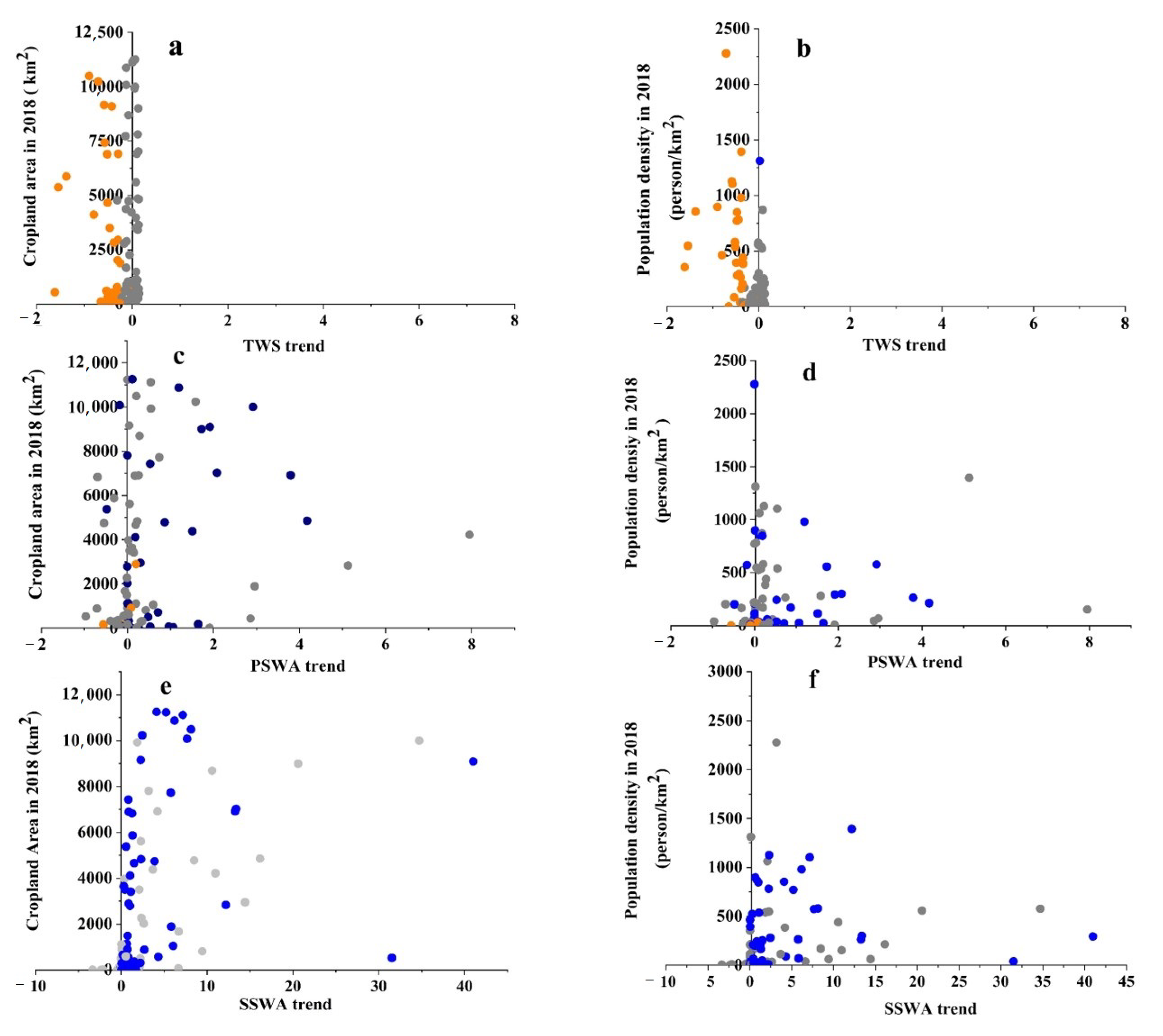
4.2. Impact of Dynamics in Water Resources on Population and Social Economy

In order to identify the potential obstacles affecting the population and economic advancement within the CPEC, we delved deeper into the changes in population distribution and cultivated land allocation over time and space in the CPEC region. According to GPW statistics, the population of the CPEC has been steadily increasing over the past few decades (Figure 10), leading to a higher demand for water resources [40]. We found that, in 2018, the total cropland area in the CPEC was approximately 3.02 × 10⁵ km2 (Figure 10c), with irrigated areas accounting for 21.05% of it. Cropland is mainly distributed in Sindh and Punjab (Figure 10c). However, TWS in Sindh decreased at a rate of 0.12 cm/year, and TWS in Punjab decreased at a rate of 0.48 cm/year. This indicates that the water resource crisis in these two areas is likely to intensify, which is consistent with the findings of Aqil Tariq [41] and Waseem Ishaque [40]. Pakistan’s agricultural sector contributed 21% to the country’s economy, with an annual growth of 2.7%, surpassing industries, which indicates an agrarian economic stage [42]. Therefore, dynamic changes in water resources not only affect the population’s use of water resources but also affect agricultural development, thereby affecting social and economic development.
In order to further analyze the impacts of water resource changes on population and cropland, we further developed the study from three perspectives, PSWA, SSWA, and TWS, based on the pixel scale (Figure 11). We found that regions with high cropland were mostly situated in areas where TWS had been severely depleted (Figure 11a), and regions with high population density were also primarily located in regions with depleted TWS (Figure 11b). Moreover, it was observed that large areas of cropland were concentrated in regions with only marginal increases in the PWSA (Figure 11c). Conversely, areas with high population density were mainly found in regions with relatively small, yet significant, increases in the PWSA (Figure 11d). Additionally, regions with substantial cropland areas were predominantly distributed in areas with a small, yet significant, seasonal increase in the SWA (Figure 11e). Lastly, high population density areas were found in areas with a small, but noteworthy, increase in the SSWA (Figure 11f). In summary, the significant decrease in TWS primarily occurred in areas of high cropland and high population density, suggesting that water resource utilization in these areas may be under considerable pressure. Furthermore, although the increases in the PWSA and SSWA are small, they still have significant implications for improving the water resource conditions in cropland and densely populated areas [43]. This indicates that even slight increases in water resources are critical for maintaining regional water balance and supporting agricultural production. Therefore, this study underscores the importance of managing and protecting water resources to ensure the sustainable development of both populations and agriculture.
Additionally, over the past few decades, research on the dynamic of water resources in the CPEC has primarily focused on the unsustainable use and management of these resources, as well as the impact of climate change [44,45,46,47,48]. These studies investigated the impacts of these variables on bodies of water from a one-dimensional angle. In fact, changes in water bodies are frequently instigated by the interplay of numerous factors [6,32]. However, it has not been given sufficient attention in the existing research on the CPEC. By neglecting the interconnected nature of these factors, the understanding of the complexity of spatial–temporal dynamics of water may be limited. In this study, we identified mainly two types of effect, a dual-factor enhancement and the nonlinear weakening of single factors (Figure 8). This finding reminds us that, to fully understand and predict water resource dynamics and their spatial–temporal complexity, the interconnectedness of these factors must be taken into account for actual management. Therefore, we suggest that future research should not only focus on the impact of a single factor on water bodies but should also pay more attention to the interaction and overall impact of multiple factors. This approach can not only help us better understand the changing dynamics of water resources in the CPEC region but also develop more effective water resource management and protection strategies.

4.3. Water Crisis in the CPEC

Pakistan, ranked third by the International Monetary Fund, faces severe water shortages. The Pakistan Council of Research in Water Resources predicts very limited access to clean water by 2025 [49]. Although the SWA showed an increasing trend, TWS witnessed a decreasing trend in most regions of the CPEC (Figure 3 and Figure 4). In addition, it can be observed that the decreasing degree of total water availability exacerbated the declining trend of water crisis in the CPEC. Pakistan is an agricultural country, and most of the water used for agriculture is extracted from groundwater [50]. The decline in TWS could indicate a decrease in groundwater [51], which could impact food security and agricultural production. Furthermore, the decline in groundwater levels could lead to the drying up of wetlands and rivers that depend on groundwater recharge, destroying ecosystems and affecting biodiversity. Such negative outcomes may lead to soil drying and salinization, exacerbating land degradation and desertification problems. Furthermore, glaciers in Pakistan are melting at a rate quicker than any other region globally as a result of the warming climate, leading to a situation in which, by the year 2035, there will be a complete absence of glaciers within the country. The increasing melting of glaciers could lead to a large SWA in a short time; however, it can result in a shortage of water resources in the CPEC in the long run [52]. Pakistan is at risk of high concentrations of arsenic in its drinking water [53]. This contradicts the United Nations’ 2015 statement of Sustainable Development Goals, one of which is to ensure that all people have access to sanitary facilities and clean, safe drinking water (Goal 6). The main reasons for the underutilization of surface water resources in Pakistan are the uneven spatial distribution of these resources over time, as well as issues with water resource management, aging infrastructure canals, and low water efficiency [49,53,54].
Pakistan’s available water resources face significant pressure due to population growth, competition for water among different sectors, climate change, and the degradation of ecosystem services caused by inadequate planning and management [40]. This presents a significant risk to the natural environment, economic and social advancement [55], and public well-being [49]. In order to promote the long-term use of water supplies within the framework of the CPEC, a variety of actions must be taken. According to our research (Figure 6 and Figure 7), Azad Kashmir and Punjab should focus on addressing population growth and maximizing the utilization of precipitation. Additionally, Kashi should consider population growth and the expansion of cropland areas. Sindh should prioritize expanding the area of cropland. Moreover, actions consist of the deployment of water-conserving technologies to enhance irrigation effectiveness; the holistic consideration of SWA, groundwater, and TWS; and fostering collaboration between nations to guarantee enduring water consumption within the CPEC and aid in attaining Sustainable Development Goal 6. It is also important to note that India’s plan to construct a dam on a tributary of the Indus River within its borders has created new tensions, as it would grant India greater control over the river’s flow.

5. Conclusions

This study identified changes in TWS and the SWA in the CPEC and explored the relationship between TWS changes and its driving factors based on geographical detectors. The following key findings were derived:
(1) Over the last two decades, CPEC regions experienced divergent water body changes: The SWA generally increased, with Sindh seeing the highest rise. Punjab’s TWS significantly decreased by −0.48 cm/year, with similar declines in Azad Kashmir. Despite some TWS increases in Khyber Pakhtunkhwa and FATA, these were not enough to counteract overall TWS reductions within the CPEC.
(2) Correlation analysis revealed that the SWA and climate change were the primary factors influencing TWS changes in Balochistan, while FATA changes were mainly influenced by climate change. On the other hand, human activities had a primary impact on TWS changes in Azad Kashmir, Punjab, and Sindh.
(3) The results of the geographical detector analysis indicated that the main interaction factors influencing TWS changes in the CPEC were primarily a dual-factor enhancement and the nonlinear weakening of single factors.
Our research further shows that although the water resources in the CPEC are increasing, the problem of declining water reserves is serious. The current population and cultivated land are mostly distributed in areas with severely declining TWS, especially Sindh and Punjab. Pakistan should address the problems faced by these two provinces. If the water crisis worsens the problem, countermeasures should be taken in advance, such as controlling rapid population growth and appropriately reducing the area of cropland.

Author Contributions

J.B. and X.H. conceptualized the study and wrote the manuscript. T.L., T.Y., G.L. and S.N. carried out data collection and analysis. J.J. and S.Y. made valuable contributions to the analysis. Y.W., P.Q., Y.Y., T.W., P.Z. and V.N. contributed to the manuscript review. All authors have read and agreed to the published version of the manuscript.

Funding

This research was funded by the Key R&D Program of Xinjiang Uygur Autonomous Region (Grant No. 2022B03021), the Tianshan Talent Training Program of Xinjiang Uygur Autonomous Region (Grant No. 2022TSYCLJ0011); and the Open Fund of the State Key Laboratory of Desert and Oasis.

Data Availability Statement

The Global Reservoir and Dam (GRanD) database v1.360 was downloaded from its website (https://www.globaldamwatch.org/grand/ (accessed on 4 March 2024)). Terrestrial water storage data based on the Gravity Recovery and Climate Experiment (GRACE TWS) were downloaded from CSR and JPL websites (CSR: http://www2.csr.utexas.edu/grace/asdp.html (accessed on 4 March 2024) and JPL: https://podaac.jpl.nasa.gov/dataset/TELLUS_GRAC-GRFO_MASCON_CRI_GRID_RL06_V2.Gldas (accessed on 4 March 2024)). The SPEI was downloaded from its website (http://sac.csic.es/spei/ (accessed on 4 March 2024)). The data for the SWA were obtained from https://global-surface-water.appspot.com (accessed on 4 March 2024). MOD16A2, an 8-day composite evapotranspiration product generating models at 500 m pixel resolution (version 6, https://lpdaacsvc.cr.usgs.gov/appeears/task/area (accessed on 4 March 2024)), was used for calculations. ERA5 is the latest generation of global reanalysis dataset produced by the European Centre for Medium-Range Weather Forecasts, and it can be downloaded from https://cds.climate.copernicus.eu/cdsapp#!/dataset/reanalysis-era5-land-monthly means?tab = form (accessed on 4 March 2024). The Gridded Population of the World dataset produced by the Population Division of the Department of Economic and Social Affairs of the United Nations Secretariat was used (https://www.worldpop.org/geodata/listing?id=77 (accessed on 4 March 2024)). The cropland area was calculated by the CCI Land Cover data (https://2018mexicolandcover10m.esa.int/download (accessed on 4 March 2024)).

Conflicts of Interest

The authors declare no conflicts of interest.

References

  1. Wang, X.; Xiao, X.; Zou, Z.; Dong, J.; Li, B. Gainers and losers of surface and terrestrial water resources in China during 1989–2016. Nat. Commun. 2020, 11, 3471. [Google Scholar] [CrossRef]
  2. Gao, Z.; Zhou, Y.; Cui, Y.; Dong, J.; Wang, X.; Zhao, G.; Zou, Z.; Xiao, X. Rebound of surface and terrestrial water resources in Mongolian plateau following sustained depletion. Ecol. Indic. 2023, 156, 111193. [Google Scholar] [CrossRef]
  3. Burlacu, S.; Vasilache, P.C.; Velicu, E.R.; Curea, Ș.-C.; Margina, O. Management of water resources at global level. In Proceedings of the International Conference on Economics and Social Sciences, Singapore, 25–26 July 2020. [Google Scholar]
  4. Zhou, Y.; Dong, J.; Cui, Y.; Zhao, M.; Wang, X.; Tang, Q.; Zhang, Y.; Zhou, S.; Metternicht, G.; Zou, Z. Ecological restoration exacerbates the agriculture-induced water crisis in North China Region. Agric. For. Meteorol. 2023, 331, 109341. [Google Scholar] [CrossRef]
  5. Huang, W.; Duan, W.; Chen, Y. Rapidly declining surface and terrestrial water resources in Central Asia driven by socio-economic and climatic changes. Sci. Total Environ. 2021, 784, 147193. [Google Scholar] [CrossRef] [PubMed]
  6. Huang, W.; Duan, W.; Nover, D.; Sahu, N.; Chen, Y. An integrated assessment of surface water dynamics in the Irtysh River Basin during 1990–2019 and exploratory factor analyses. J. Hydrol. 2021, 593, 125905. [Google Scholar] [CrossRef]
  7. Kahil, M.T.; Dinar, A.; Albiac, J. Modeling water scarcity and droughts for policy adaptation to climate change in arid and semiarid regions. J. Hydrol. 2015, 522, 95–109. [Google Scholar] [CrossRef]
  8. Stringer, L.C.; Mirzabaev, A.; Benjaminsen, T.A.; Harris, R.M.; Jafari, M.; Lissner, T.K.; Stevens, N.; Tirado-von Der Pahlen, C. Climate change impacts on water security in global drylands. One Earth 2021, 4, 851–864. [Google Scholar] [CrossRef]
  9. Wasko, C.; Nathan, R.; Stein, L.; O’Shea, D. Evidence of shorter more extreme rainfalls and increased flood variability under climate change. J. Hydrol. 2021, 603, 126994. [Google Scholar] [CrossRef]
  10. Leal Filho, W.; Totin, E.; Franke, J.A.; Andrew, S.M.; Abubakar, I.R.; Azadi, H.; Nunn, P.D.; Ouweneel, B.; Williams, P.A.; Simpson, N.P. Understanding responses to climate-related water scarcity in Africa. Sci. Total Environ. 2022, 806, 150420. [Google Scholar] [CrossRef]
  11. Khandu; Forootan, E.; Schumacher, M.; Awange, J.L.; Mueller Schmied, H. Exploring the influence of precipitation extremes and human water use on total water storage (TWS) changes in the G anges-B rahmaputra-M eghna River Basin. Water Resour. Res. 2016, 52, 2240–2258. [Google Scholar] [CrossRef]
  12. Ruan, H.; Yu, J.; Wang, P.; Wang, T. Increased crop water requirements have exacerbated water stress in the arid transboundary rivers of Central Asia. Sci. Total Environ. 2020, 713, 136585. [Google Scholar] [CrossRef] [PubMed]
  13. Lian, X.; Piao, S.; Chen, A.; Huntingford, C.; Fu, B.; Li, L.Z.; Huang, J.; Sheffield, J.; Berg, A.M.; Keenan, T.F. Multifaceted characteristics of dryland aridity changes in a warming world. Nat. Rev. Earth Environ. 2021, 2, 232–250. [Google Scholar] [CrossRef]
  14. Liu, X.; Liu, Y.; Wang, Y.; Liu, Z. Evaluating potential impacts of land use changes on water supply–demand under multiple development scenarios in dryland region. J. Hydrol. 2022, 610, 127811. [Google Scholar] [CrossRef]
  15. Rocha, J.; Carvalho-Santos, C.; Diogo, P.; Beça, P.; Keizer, J.J.; Nunes, J.P. Impacts of climate change on reservoir water availability, quality and irrigation needs in a water scarce Mediterranean region (southern Portugal). Sci. Total Environ. 2020, 736, 139477. [Google Scholar] [CrossRef]
  16. kumar Nayan, N.; Das, A.; Mukerji, A.; Mazumder, T.; Bera, S. Spatio-temporal dynamics of water resources of Hyderabad Metropolitan Area and its relationship with urbanization. Land Use Policy 2020, 99, 105010. [Google Scholar] [CrossRef]
  17. An, L.; Wang, J.; Huang, J.; Pokhrel, Y.; Hugonnet, R.; Wada, Y.; Cáceres, D.; Müller Schmied, H.; Song, C.; Berthier, E. Divergent causes of terrestrial water storage decline between drylands and humid regions globally. Geophys. Res. Lett. 2021, 48, e2021GL095035. [Google Scholar] [CrossRef]
  18. Zhao, M.; Zhang, J.; Velicogna, I.; Liang, C.; Li, Z. Ecological restoration impact on total terrestrial water storage. Nat. Sustain. 2020, 4, 56–62. [Google Scholar] [CrossRef]
  19. Meng, F.; Su, F.; Li, Y.; Tong, K. Changes in Terrestrial Water Storage During 2003–2014 and Possible Causes in Tibetan Plateau. J. Geophys. Res. Atmos. 2019, 124, 2909–2931. [Google Scholar] [CrossRef]
  20. Wang, J.; Song, C.; Reager, J.T.; Yao, F.; Famiglietti, J.S.; Sheng, Y.; MacDonald, G.M.; Brun, F.; Schmied, H.M.; Marston, R.A.; et al. Recent global decline in endorheic basin water storages. Nat. Geosci. 2018, 11, 926–932. [Google Scholar] [CrossRef]
  21. Humphrey, V.; Rodell, M.; Eicker, A. Using Satellite-Based Terrestrial Water Storage Data: A Review. Surv. Geophys. 2023, 44, 1489–1517. [Google Scholar] [CrossRef]
  22. Rodell, M.; Famiglietti, J.S.; Wiese, D.N.; Reager, J.T.; Beaudoing, H.K.; Landerer, F.W.; Lo, M.H. Emerging trends in global freshwater availability. Nature 2018, 557, 651–659. [Google Scholar] [CrossRef] [PubMed]
  23. Taheri Dehkordi, A.; Valadan Zoej, M.J.; Ghasemi, H.; Jafari, M.; Mehran, A. Monitoring Long-Term Spatiotemporal Changes in Iran Surface Waters Using Landsat Imagery. Remote Sens. 2022, 14, 4491. [Google Scholar] [CrossRef]
  24. Zhao, Z.; Li, H.; Song, X.; Sun, W. Dynamic Monitoring of Surface Water Bodies and Their Influencing Factors in the Yellow River Basin. Remote Sens. 2023, 15, 5157. [Google Scholar] [CrossRef]
  25. Borja, S.; Kalantari, Z.; Destouni, G. Global Wetting by Seasonal Surface Water Over the Last Decades. Earth’s Future 2020, 8, e2019EF001449. [Google Scholar] [CrossRef]
  26. Pekel, J.-F.; Cottam, A.; Gorelick, N.; Belward, A.S. High-resolution mapping of global surface water and its long-term changes. Nature 2016, 540, 418–422. [Google Scholar] [CrossRef] [PubMed]
  27. An, N.; Mustafa, F.; Bu, L.; Xu, M.; Wang, Q.; Shahzaman, M.; Bilal, M.; Ullah, S.; Feng, Z. Monitoring of atmospheric carbon dioxide over Pakistan using satellite dataset. Remote Sens. 2022, 14, 5882. [Google Scholar] [CrossRef]
  28. Faiz, M.A.; Liu, D.; Tahir, A.A.; Li, H.; Fu, Q.; Adnan, M.; Zhang, L.; Naz, F. Comprehensive evaluation of 0.25° precipitation datasets combined with MOD10A2 snow cover data in the ice-dominated river basins of Pakistan. Atmos. Res. 2020, 231, 104653. [Google Scholar] [CrossRef]
  29. Ashiq, M.W.; Zhao, C.; Jian, N.; Akhtar, M. GIS-based high-resolution spatial interpolation of precipitation in mountain–plain areas of Upper Pakistan for regional climate change impact studies. Theor. Appl. Climatol. 2010, 99, 239–253. [Google Scholar] [CrossRef]
  30. Iqbal, M.F.; Athar, H. Validation of satellite based precipitation over diverse topography of Pakistan. Atmos. Res. 2018, 201, 247–260. [Google Scholar] [CrossRef]
  31. Save, H.; Bettadpur, S.; Tapley, B.D. High-resolution CSR GRACE RL05 mascons. J. Geophys. Res. Solid Earth 2016, 121, 7547–7569. [Google Scholar] [CrossRef]
  32. Qi, P.; Huang, X.; Xu, Y.J.; Li, F.; Wu, Y.; Chang, Z.; Li, H.; Zhang, W.; Jiang, M.; Zhang, G. Divergent trends of water bodies and their driving factors in a high-latitude water tower, Changbai Mountain. J. Hydrol. 2021, 603, 127094. [Google Scholar] [CrossRef]
  33. Qian, A.; Yi, S.; Chang, L.; Sun, G.; Liu, X. Using GRACE Data to Study the Impact of Snow and Rainfall on Terrestrial Water Storage in Northeast China. Remote Sens. 2020, 12, 4166. [Google Scholar] [CrossRef]
  34. Busker, T.; Roo, A.D.; Gelati, E.; Schwatke, C.; Cottam, A. A global lake and reservoir volume analysis using a surface water dataset and satellite altimetry. Hydrol. Earth Syst. Sci. 2019, 23, 669–690. [Google Scholar] [CrossRef]
  35. Thorslund, J.; Vliet, M. A global dataset of surface water and groundwater salinity measurements from 1980–2019. Sci. Data 2020, 7, 231. [Google Scholar] [CrossRef] [PubMed]
  36. Beguería, S.; Vicente-Serrano, S.M.; Reig, F.; Latorre, B. Standardized precipitation evapotranspiration index (SPEI) revisited: Parameter fitting, evapotranspiration models, tools, datasets and drought monitoring. Int. J. Climatol. 2014, 34, 3001–3023. [Google Scholar] [CrossRef]
  37. Wang, J.-F.; Zhang, T.-L.; Fu, B.-J. A measure of spatial stratified heterogeneity. Ecol. Indic. 2016, 67, 250–256. [Google Scholar] [CrossRef]
  38. Song, Y.; Wang, J.; Ge, Y.; Xu, C. An optimal parameters-based geographical detector model enhances geographic characteristics of explanatory variables for spatial heterogeneity analysis: Cases with different types of spatial data. GIScience Remote Sens. 2020, 57, 593–610. [Google Scholar] [CrossRef]
  39. Zhu, L.; Meng, J.; Zhu, L. Applying Geodetector to disentangle the contributions of natural and anthropogenic factors to NDVI variations in the middle reaches of the Heihe River Basin. Ecol. Indic. 2020, 117, 106545. [Google Scholar] [CrossRef]
  40. Ishaque, W.; Mukhtar, M.; Tanvir, R. Pakistan’s water resource management: Ensuring water security for sustainable development. Front. Environ. Sci. 2023, 11, 1096747. [Google Scholar] [CrossRef]
  41. Tariq, A.; Qin, S. Spatio-temporal variation in surface water in Punjab, Pakistan from 1985 to 2020 using machine-learning methods with time-series remote sensing data and driving factors. Agric. Water Manag. 2023, 280, 108228. [Google Scholar] [CrossRef]
  42. Azam, A.; Shafique, M. Agriculture in Pakistan and its Impact on Economy. A Review. Int. J. Adv. Sci. Technol. 2017, 103, 47–60. [Google Scholar] [CrossRef]
  43. Siyal, A.W.; Gerbens-Leenes, P.W.; Nonhebel, S. Energy and carbon footprints for irrigation water in the lower Indus basin in Pakistan, comparing water supply by gravity fed canal networks and groundwater pumping. J. Clean. Prod. 2021, 286, 125489. [Google Scholar] [CrossRef]
  44. Dars, G.H.; Najafi, M.R.; Qureshi, A.L. Assessing the Impacts of Climate Change on Future Precipitation Trends Based on Downscaled CMIP5 Simulations Data. Mehran Univ. Res. J. Eng. Technol. 2017, 36, 385–394. [Google Scholar] [CrossRef]
  45. Immerzeel, W.W.; Beek Van, L.P.H.; Bierkens, M.F.P. Climate change will affect the Asian water towers. Science 2010, 328, 1382–1385. [Google Scholar] [CrossRef] [PubMed]
  46. Lutz, A.F.; Immerzeel, W.W.; Shrestha, A.B.; Bierkens, M.F.P. Consistent increase in High Asia’s runoff due to increasing glacier melt and precipitation. Nat. Clim. Chang. 2014, 4, 587–592. [Google Scholar] [CrossRef]
  47. Siddiqi, A.; Wescoat, J.L.; Muhammad, A. Socio-hydrological assessment of water security in canal irrigation systems: A conjoint quantitative analysis of equity and reliability. Water Secur. 2018, 4, 44–55. [Google Scholar] [CrossRef]
  48. Wescoat, J.L.; Siddiqi, A.; Muhammad, A. Socio-Hydrology of Channel Flows in Complex River Basins: Rivers, Canals, and Distributaries in Punjab, Pakistan. Water Resour. Res. 2018, 54, 464–479. [Google Scholar] [CrossRef]
  49. Nabi, G.; Ali, M.; Khan, S.; Kumar, S. The crisis of water shortage and pollution in Pakistan: Risk to public health, biodiversity, and ecosystem. Environ. Sci. Pollut. Res. 2019, 26, 10443–10445. [Google Scholar] [CrossRef] [PubMed]
  50. Kirby, M.; Mainuddin, M.; Khaliq, T.; Cheema, M. Agricultural production, water use and food availability in Pakistan: Historical trends, and projections to 2050. Agric. Water Manag. 2017, 179, 34–46. [Google Scholar] [CrossRef]
  51. MacAllister, D.; Krishan, G.; Basharat, M.; Cuba, D.; MacDonald, A. A century of groundwater accumulation in Pakistan and northwest India. Nat. Geosci. 2022, 15, 390–396. [Google Scholar] [CrossRef]
  52. Mustafa, U.; Baig, M.B.; Straquadine, G.S. Impacts of Climate Change on Agricultural Sector of Pakistan: Status, Consequences, and Adoption Options. Emerg. Chall. Food Prod. Secur. Asia Middle East Afr. Clim. Risks Resour. Scarcity 2021, 2021, 43–64. [Google Scholar]
  53. Zeb, H.; Yaqub, A.; Ajab, H.; Zeb, I.; Khan, I. Effect of Climate Change and Human Activities on Surface and Ground Water Quality in Major Cities of Pakistan. Water 2023, 15, 2693. [Google Scholar] [CrossRef]
  54. Yasin, H.Q.; Breadsell, J.; Tahir, M.N. Climate-water governance: A systematic analysis of the water sector resilience and adaptation to combat climate change in Pakistan. Water Policy 2021, 23, 1–35. [Google Scholar] [CrossRef]
  55. Rehman, I.; Ishaq, M.; Ali, L.; Khan, S.; Ahmad, I.; Din, I.U.; Ullah, H. Enrichment, spatial distribution of potential ecological and human health risk assessment via toxic metals in soil and surface water ingestion in the vicinity of Sewakht mines, district Chitral, Northern Pakistan. Ecotoxicol. Environ. Saf. 2018, 154, 127–136. [Google Scholar] [CrossRef] [PubMed]
Figure 1. Geographical location of the China–Pakistan Economic Corridor as well as the spatial distribution of the elevation, river network, and dams within the study area.
Remotesensing 16 01437 g001
Figure 2. The interaction type between two independent variables. (Min(q(X1), q(X2) means to find the minimum value between q(X1) and q(X2); Max(q(X1), q(X2)) means to find the maximum value between q(X1) and q(X2); q(X1∩X2) means q(X1), q(X2) is interactive; q(X1) + q(X2) is used to calculate the sum of q(X1) and q(X2)). In our study, SWA and TWS were classified as attributes, whereas the cropland area, the surface area of the dam, annual evaporation, population density, annual precipitation, and the annual average temperature were identified as factors.
Remotesensing 16 01437 g002
Figure 3. Interannual variations and trends of annual SWA during 2002–2018 in the CPEC: (ac) the SWA per unit land (km2), changes in the slope of SWA, and the significance level of the SWA change, respectively.
Remotesensing 16 01437 g003
Figure 4. Interannual variations and trends in terrestrial water storage from 2002 to 2018: (a) the slope of TWS; (b) the significance level of TWS change trend.
Remotesensing 16 01437 g004
Figure 5. The linear regression trends between TWS and SWA in the CPEC from 2002 to 2018: (a) the linear regression trends between TWS and SWA; (b) the R square of linear regression trends between TWS and SWA.
Remotesensing 16 01437 g005
Figure 6. The correlation coefficient between TWS and driving factors in the CPEC: ** and * refer to the significant level with p < 0.01 and p < 0.05, respectively. CROP refers to the area of cropland, DAM represents the surface area of the dam, EVA represents the annual evaporation, POP represents population density, PRE represents annual precipitation, and TEM represents the annual average temperature.
Remotesensing 16 01437 g006
Figure 7. The contribution of driving factors to TWS changes in the CPEC (the wider the line, the greater the weight): CROP represents the area of cropland, EVA represents the annual evaporation, POP represents population density, PRE represents annual precipitation, and TEM represents the annual average temperature.
Remotesensing 16 01437 g007
Figure 8. Contributions of driving factors interaction to TWS in the CPEC: (a) Azad Kashmir; (b) Balochistan; (c) FATA; (d) Gilgit-Baltistan; (e) Kashi; (f) Sindh; (g) Khyber Pakhtunkhwa; (h) Punjab. CROP represents the area of cropland, EVA represents the annual evaporation, POP represents population density, PRE represents annual precipitation, and TEM represents the annual average temperature.
Remotesensing 16 01437 g008
Figure 9. SWA, TWS, and the Standardized Precipitation–Evapotranspiration Index: (a) Azad Kashmir; (b) Balochistan; (c) FATA; (d) Gilgit–Baltistan; (e) Kashi; (f) Sindh; (g) Khyber Pakhtunkhwa; (h) Punjab. The SPEI is the Standardized Precipitation–Evapotranspiration Index. The dashed lines indicate the dam’s construction year.
Remotesensing 16 01437 g009
Figure 10. Trends of population density in Central Asia at the national scale from the fourth version of the Gridded Population of the World from 2002 to 2018: (a) the density of population; (b) the significance level of the population density change trend; (c) spatial distribution of land cover types in 2018: 10: cropland (rainfed), 20: cropland (irrigated or post-flooding), 30: mosaic cropland–natural vegetation (coverage rate greater than 50% natural vegetation (tree, shrub, and herbaceous cover) and less than 50% cropland).
Remotesensing 16 01437 g010
Figure 11. The relationships between TWS trends, PSWA trends, SSWA trends, population density in 2018, and cropland area in 2018 at the 0.5° grid scale. (a) TWS trend and the cropland area in 2018; (b) TWS trend and the cropland area in 2018; (c) PSWA trend and the population density in 2018; (d) PSWA trend and the population density in 2018; (e) SSWA trend and thr cropland area in 2018; (f) SSWA trend and the population density in 2018.
Remotesensing 16 01437 g011
Table 1. The missing data of GRACE from 2002 to 2018.
YearMonth
200212367
20036
20111612
2012510
2013389
20142712
2015561011
20164910
20172789101112
20181234589
Table 2. Characteristics and construction details of the dams in the CPEC.
RegionDam NameConstruction YearDam HeightArea (km2)
FATAGomal Zam201313335.97
SindhDarawat2013468.93
Gilgit–BaltistanSatpara2011393.21
BalochistanMirani20073962.95
Disclaimer/Publisher’s Note: The statements, opinions and data contained in all publications are solely those of the individual author(s) and contributor(s) and not of MDPI and/or the editor(s). MDPI and/or the editor(s) disclaim responsibility for any injury to people or property resulting from any ideas, methods, instructions or products referred to in the content.

