
Object-Based Semi-Supervised Spatial Attention Residual UNet for Urban High-Resolution Remote Sensing Image Classification


1
State Key Laboratory of Black Soils Conservation and Utilization, Northeast Institute of Geography and Agroecology, Chinese Academy of Sciences, Changchun 130102, China
2
University of Chinese Academy of Sciences, Beijing 100049, China
3
State Key Laboratory of Remote Sensing Science, Aerospace Information Research Institute, Chinese Academy of Sciences, Beijing 100094, China
4
School of Geographical Sciences, University of Bristol, Bristol BS8 1SS, UK
*
Author to whom correspondence should be addressed.
Remote Sens. 2024, 16(8), 1444; https://doi.org/10.3390/rs16081444
Submission received: 19 February 2024
/
Revised: 9 April 2024
/
Accepted: 15 April 2024
/
Published: 18 April 2024
(This article belongs to the Special Issue Advanced Artificial Intelligence for Environmental Remote Sensing)
Abstract
:Accurate urban land cover information is crucial for effective urban planning and management. While convolutional neural networks (CNNs) demonstrate superior feature learning and prediction capabilities using image-level annotations, the inherent mixed-category nature of input image patches leads to classification errors along object boundaries. Fully convolutional neural networks (FCNs) excel at pixel-wise fine segmentation, making them less susceptible to heterogeneous content, but they require fully annotated dense image patches, which may not be readily available in real-world scenarios. This paper proposes an object-based semi-supervised spatial attention residual UNet (OS-ARU) model. First, multiscale segmentation is performed to obtain segments from a remote sensing image, and segments containing sample points are assigned the categories of the corresponding points, which are used to train the model. Then, the trained model predicts class probabilities for all segments. Each unlabeled segment’s probability distribution is compared against those of labeled segments for similarity matching under a threshold constraint. Through label propagation, pseudo-labels are assigned to unlabeled segments exhibiting high similarity to labeled ones. Finally, the model is retrained using the augmented training set incorporating the pseudo-labeled segments. Comprehensive experiments on aerial image benchmarks for Vaihingen and Potsdam demonstrate that the proposed OS-ARU achieves higher classification accuracy than state-of-the-art models, including OCNN, 2OCNN, and standard OS-U, reaching an overall accuracy (OA) of 87.83% and 86.71%, respectively. The performance improvements over the baseline methods are statistically significant according to the Wilcoxon Signed-Rank Test. Despite using significantly fewer sparse annotations, this semi-supervised approach still achieves comparable accuracy to the same model under full supervision. The proposed method thus makes a step forward in substantially alleviating the heavy sampling burden of FCNs (densely sampled deep learning models) to effectively handle the complex issue of land cover information identification and classification.
1. Introduction
As the rapid expansion of urban areas continues worldwide, timely and accurate mapping of land cover dynamics provides vital information for sustainable development and management [1,2,3]. Compared to traditional ground-based surveys, remote sensing enables efficient large-area coverage at flexible repeated intervals [4]. In recent years, the number of remote sensing satellites has surged dramatically, providing massive geographic imagery for almost every corner of the Earth’s surface [5,6]. In extracting urban land cover information from remote sensing data, researchers often consider spatial resolution more important than spectral resolution [7,8]. This is because spatial resolution can reflect the shape and texture features of objects, for example, roads and buildings have similar spectral features but different shape and texture features [9,10,11], which can be used to distinguish these two types of objects. However, compared to the mixed effects of medium-low spatial resolution sensors, the increased within-scene spectral variability of high spatial resolution sensors may reduce the pixel-based classification accuracy of conventional approaches [12].
To address this challenge, object-based image analysis (OBIA) techniques emerged as a promising alternative in a timely manner [13]. OBIA first utilizes the multiscale characteristics of different geo-objects in high-resolution imagery to segment an image into a series of adjacent homogeneous regions (i.e., segments) of pixel sets, then fully exploits spectral, textural, shape, semantic, and other features, mining the spatial dimensions (distance, pattern, neighborhood, and topology) of segments to further aggregate them into objects to ensure classification accuracy [14]. In this process, the most basic processing unit is the segment rather than the pixel, thus avoiding the “salt-and-pepper” phenomenon of pixel-based methods. OBIA has gained rapid recognition in the remote sensing field, marked by a focus on object semantics explored through fixed or emerging ontologies, as well as the need for interoperability between OBIA approaches and geographic information systems (GIS) along with spatial modeling frameworks [15,16,17]. The above advantages have made the OBIA method gradually evolve into a new paradigm for high-resolution remote sensing and spatial analysis [13]. Traditional machine learning classification models based on object-based methods usually take the statistical summary of all pixels in a segment as input. However, with the increase in image resolution, the spectral heterogeneity within objects and the homogeneity between objects are both increasing, which makes such summarization inevitably carry noise, thus eventually leading to misclassification [18,19]. To overcome this problem, it is necessary to introduce additional morphological and textural information of segments into the classification process [20,21]. However, these feature engineering methods typically rely on prior human knowledge, which often introduces subjectivity into the process [22].
In recent years, deep learning technology has made breakthrough progress in the field of computer vision [23]. In particular, convolutional neural networks (CNNs) can automatically extract high-level features from image patches through a series of convolutional and pooling layers and have demonstrated excellent representation and classification capabilities for object shape, texture, and context information [24,25]. These methods thus avoid the tedious and time-consuming hand-crafted feature engineering required in traditional remote sensing image analysis methods [26]. Therefore, it is necessary to combine object-based image analysis with deep learning methods to take advantage of each. Initially, CNNs were applied to remote sensing image scene classification, where rectangular patches cropped from images were fed into the CNNs, which then output an image-level label [27,28,29]. In full-resolution remote sensing mapping, however, densely overlapping patches are used pixel by pixel, which inevitably leads to extremely redundant computation [30]. To address this issue, CNNs with objects as the basic processing units can better preserve the boundaries of geographical entities, reduce computational cost, and improve processing efficiency [30]. However, in remote sensing images, the distribution range of the central target area to be classified may be relatively small while background information occupies larger areas. Therefore, classification is inevitably affected by heterogeneous content, which leads to the wrong classification of regions of interest into background categories [28]. Currently, the common strategy is to use an ensemble of models with different input scales to suppress heterogeneity and enhance feature representation capability for the central region. However, these methods require comprehensive consideration of inter-model scale combinations, parameter relations, and sample distributions [31,32,33,34], and it is thus relatively complex to apply them in practice.
Fully convolutional networks (FCNs) can achieve dense pixel-level prediction and are not affected by the content heterogeneity of image patches [35]. Therefore, FCNs and their extensions have been gradually introduced into remote sensing semantic segmentation [30,34]. The main difference between CNNs and fully convolutional networks (FCNs) is that FCNs replace the fully connected layers in CNNs with convolutional layers [35]. This enables FCNs to take images of arbitrary sizes as input and generate correspondingly sized output segmentation maps, thereby achieving dense pixel-level prediction. Representative FCN models include SegNet [36], U-Net [37], Deeplab series [38,39,40], PSPNet [41], DenseASPP [42], DANet [43], OCNet [44], and, more recently, UNet++ [45] and Auto-DeepLab [46]. These FCNs are commonly pre-trained on large-scale natural image datasets like ImageNet, then finetuned on remote sensing images to mitigate overfitting caused by limited labeled training samples [47,48]. Multiscale feature integration through pyramid pooling modules [41] or encoder–decoder structures [37] helps FCNs capture both local details and global context. Conditional random fields (CRFs) can further refine object boundaries as a post-processing step [39]. Atrous/dilated convolutions maintain large receptive fields without losing resolution [38]. Attention mechanisms focus models on informative regions and reduce confusion due to irrelevant features [49]. However, several issues remain to be addressed for remote sensing FCN segmentation, such as large intra-class variance, small inter-class differences, and the lack of sufficient annotated samples.
FCNs can achieve high classification accuracy owing to abundant labeled samples and powerful computational capabilities. However, in some practical applications, it is difficult to obtain large amounts of labeled data samples. To address this issue, transfer learning provides an effective solution. The idea of transfer learning is to use publicly available pre-trained neural networks containing massive generic data as a basis, then fine-tune them on a small amount of data samples from a specific domain to alleviate overfitting caused by limited labeled training samples, thereby obtaining a well-performing neural network model [50,51]. However, most of the above methods were tested on RGB public datasets [50,51]. There are fewer specific applications on multispectral remote sensing images, which differ from natural images in terms of indistinct target boundaries, large variances in similar target sizes, small inter-class differences, large intra-class differences, and distribution differences between source domain datasets and target domain datasets. These differences make it difficult to directly transfer models pre-trained on natural images to remote sensing image segmentation tasks [52]. In addition, when there are more categories in the test dataset to be segmented than in the training dataset, transfer learning methods cannot achieve good segmentation accuracy [53].
Compared to relying on pre-trained models, models trained from scratch can better adapt to multiband target datasets. Semi-supervised learning, by reducing annotation costs, has become an effective implementation of this training paradigm. It complements a small labeled dataset with a large number of unlabeled images to improve model generalization. The main categories of semi-supervised learning include self-training, consistency regularization, generative models, graph-based methods, and, more recently, adversarial training [54,55,56,57]. Self-training is one of the earliest and most widely used semi-supervised learning strategies due to its simplicity [58]. It first trains a model on limited labeled data, then uses the model to generate pseudo-labels for unlabeled images. The unlabeled images with pseudo-labels are combined with the labeled set to retrain the model. Increasing the amount of data can prevent overfitting caused by limited data samples. Consistency regularization enforces consistent model predictions when unlabeled data are perturbed through noise injection, image flipping, cropping, etc. [59].
These semi-supervised techniques have been integrated with deep convolutional neural networks and applied to remote sensing image segmentation tasks. For example, Staeger et al. proposed a self-training method by predicting pseudo-labels from an FCN ensemble [60]. French et al. applied strong data augmentation as consistency regularization for iterative self-training [59]. Souly et al. used GANs to generate additional labeled data from unlabeled images [57]. Recent works have incorporated spatial–contextual information in graph structures as well [61,62]. More recent semi-supervised segmentation methods also include co-training, where two models provide complementary supervision for each other [63]. Curriculum learning gradually incorporates unlabeled data from easy to hard based on prediction confidence [64]. Hybrid methods combine self-training, consistency regularization, and adversarial training for improved performance [65]. Despite promising results on benchmarks like ISPRS Potsdam and Vaihingen, several issues remain to be addressed [66]. Some methods have attempted semantic segmentation of remote sensing images, but most are based on binary semantic segmentation with few categories and large inter-class differences [26]. Meanwhile, they experience problems of complex training, large computational demands, and high memory usage, and false pseudo-labeling can easily mislead self-training. Despite its potential, limited research has been done on few-shot semi-supervised learning, which remains an active area of research for reducing annotation efforts in remote sensing image segmentation.
To provide a single-model approach that can work with limited samples, this paper proposes a from-scratch-trained, object-based, semi-supervised spatial attention residual UNet (OS-ARU) for urban land cover classification of multiband high-resolution remote sensing imagery. First, segments obtained via multiscale segmentation serve as a bridge to assign known sample point categories to the segments they fall in to train the model. Then, the similarity between segments of known and unknown categories is compared based on the mean probability distribution over classes from model predictions, and unknown segments obtain pseudo-labels via label propagation. Finally, the model is retrained on the original sample set augmented with pseudo-annotation information. With such an algorithm, OS-ARU can be trained using sample sets based on sparse pixels. Therefore, it is not adversely affected by image content heterogeneity, thus simplifying its implementation and usage as a single model. Ablation experiments further demonstrate that the spatial attention and residual components bring complementary gains individually, with only slight performance drops when removed separately. Experimental results show that OS-ARU achieves the highest overall classification metrics compared to other benchmark methods and is not very sensitive to input scales. In summary, the contributions of our work are as follows:
- (1)
- A selective categorical focal loss function with label smoothing adapted for FCNs trained on incompletely annotated sample sets.
- (2)
- Object-based classification executed with a single FCN model, OS-ARU, without relying on other models to suppress heterogeneity.
- (3)
- A procedure of training FCNs using sparse pixel sample points and generating pseudo-labels, then retraining the model on the sample set augmented with pseudo-category information.
2. Methodology
2.1. The Overall Process of the Proposed Semi-Supervised Method
The FCN model requires the structure of sample data consisting of input image patches and corresponding complete dense annotated ground truth patches for training and validation. However, remote sensing images usually contain more object categories compared to natural images, which makes their annotation more time-consuming and labor-intensive. That is, it is extremely difficult to obtain sufficient densely annotated image patches to meet practical task requirements. In contrast to the difficulty of obtaining such annotated image patches, sparse point samples are relatively accessible and feasible for image classification. However, there exist difficulties and challenges in transforming pixel samples into the annotated image patch samples required by FCN models. To handle this issue, Pan et al. [28] proposed a method to assign the category of a sample point to the segment obtained by geographical object-based segmentation containing the sample point to obtain sparsely labeled image patches. However, their method is only applicable to pre-trained models, which are generally trained on three-band natural images. This paper further improves this method to make it widely suitable for multiband remote sensing data. In particular, we propose a selective categorical focal loss function with label smoothing (SCFL) suitable for semi-supervised classification with incompletely labeled training sets.
Since the majority of regions in image patches remain unlabeled based on sparse pixel samples, the issue of how to feed and train models from scratch with incompletely annotated image patches needs to be addressed. Thus, a smaller number of annotated pixels of the image patches participating in model training may fail to provide the complete distribution of categories and spatial features for model learning. In order to obtain category information for more pixels, we effectively measure the similarity between segments containing sample pixels and segments without sample pixels and generate pseudo-labels for the segments that meet the threshold through label propagation. It is worth noting that the model does not need to make a correct inference for each pixel, as long as the proportion of pixels in a segment whose categories are predicted correctly is greater than that of those whose categories are predicted incorrectly, then it is enough to obtain the correct category label for the segment. That is, the dominant labels of the pixels within a segment decide the category label of the segment, which makes it possible to train an object-based FCN model using pixel samples. In order to make full use of limited training data with incomplete annotations, this paper proposes an object-based semi-supervised spatial attention residual UNet model (OS-ARU) which combines the UNet model with residual modules and attention modules to effectively capture both local and global contextual information and focus more on the most informative parts of input images. The overall process of the method is shown in Figure 1, in which three major steps are included:
- (1)
- Construction of a patch-based sample set with sparse pixel samples (CPSSP): Suppose that a densely labeled sample set of a ground truth image is not available. A high-resolution remote sensing image, Irs, and a sparse pixel-based training sample set, Tpixel, serve as the input of this algorithm. First, image Irs is segmented into homogeneous regions to generate the segmentation result, Iseg. Due to the fact that different objects may exhibit different spatial scales, multiscale segmentation is adopted as an object-based segmentation algorithm to generate meaningful objects with geometric information [67,68]. Theoretically, each segment should explicitly belong to a single object, and the inclusion of different objects in the same segment should be avoided. The image should therefore be over-segmented. Subsequently, according to the coordinates of the samples in Tpixel, Irs is sliced into image patches to construct the initial patch-based sample set, T1patch.
- (2)
- Pseudo-label sample generation and retraining of the model: First, T1patch is fed into the created model to be trained. The pixel category information contained in the patch-based sample set is enhanced by the trained model, M, through a label propagation algorithm named “construction of a patch-based sample set with pseudo-annotation” (CPSPA, shown in Figure 1). Then, in turn, M is further trained with the enhanced sample set with pseudo-label information added. This semi-supervised method improves the capacity of the model, M, to classify objects into the corresponding categories.
- (3)
- Segment classification (SC): First, the remote sensing image Irs is cropped into a series of image patches corresponding to each segment from Iseg. Then, the model, M, is used to classify each image patch obtained above. Finally, according to the most frequent category label of the pixels in each segment, the category label for the segment is decided and recorded in the classification result image, Iresult.
2.2. Detailed Implementation Process of the OS-ARU Method
2.2.1. Initial Patch-Based Sample Set Construction
The meaning of each parameter and variable in Algorithm 1 CPSSP is explained below. Irs represents the preprocessed multiband remote sensing images. The training set, Tpixel. consists of Np sparse sample point pixels, represented by {t1, t2, …, tNp}. Each vector sample, ti, is determined by three elements, namely, a coordinatei, a valuei, and a labeli, denoting the coordinate of the sample within Irs, the multiband values of pixels, and the category, ranging from 1 to Nc (the number of categories), respectively.
Following Pan et al. [28], three steps are implemented to generate the initial patch sample set using sparse pixel samples. First, an object-based multiscale segmentation is performed on Irs to obtain a segmentation image, Iseg. Then, the segment that each pixel in image Irs belongs to is determined according to the segment ID value of the pixel at the corresponding position in image Iseg. Finally, a vector representing the category d = {d1, d2, …, dNc} is introduced to characterize the category information of each segment derived from Iseg. The vector d may occur in either of two scenarios:
- (1)
- The category label is known: When a segment S contains at least one training pixel sample, ti, it is theoretically feasible to use the label of a sample pixel to measure how segment S is represented. The di under this condition can be expressed as in the following Formula (1):
The value of di in the above formula (1) is 0 or 1: when the pixel sample label belongs to the corresponding category, the value of di is 1; otherwise, the value of di is 0.
- (2)
- The category label is unknown: When a segment, S, contains no training samples, it is unknown what type of label each pixel in S has. The di in the circumstance can be written as in the following Formula (2):
According to the above two formulas, an initial patch-based sample set with incomplete annotation is created on the basis that the category label of each segment can be represented.
An initial patch-based sample set, T1patch, is constructed by the CPSSP algorithm using each sparse pixel sample in Tpixel. Each sample in T1patch is composed of SubIx and SubIy, where SubIx is a remote sensing image patch of size W × W and SubIy is the label of the patch corresponding to SubIx. Since only a small fraction of the segments in Iseg have category information, SubIy possesses limited category labels which are not densely and completely annotated. Algorithm 1 CPSSP, below, describes the process in detail [28].
| Algorithm 1: Construction of a patch-based sample set with sparse pixel samples (CPSSP). |
| Input: Irs, Iseg, Tpixel, W |
| Output: T1patch |
| Begin |
| T1patch = Ø |
| Ilabel = create an empty image with the same length and width as Irs and a depth equal to Nc. |
| For each segment, S, in Iseg: |
| cs = the coordinates of the pixels in S |
| If S contains at least one sample, ti: |
| d = category represented as shown in Formula (1) |
| Else: |
| d = category represented as shown in Formula (2) |
| Ilabel[cs] = d |
| For each sample, ti, in Tpixel: |
| cp = the center point of the segment, S, that contains ti |
| SubIx = cut a W × W image patch from Irs with cp as center |
| SubIy = cut a W × W image patch from Ilabel with cp as center |
| T1patch ← [SubIx, SubIy] |
| Return T1patch |
| End |
2.2.2. Pseudo-Label Generation and Model Retraining
This section mainly consists of three parts. First, the OS-ARU model structure incorporating residual modules and a spatial attention module adopted in this study, which is intended to capture discriminative features from limited annotated pixels, is described in detail; second, the CPSPA algorithm for generating pseudo-label sample patches based on sparsely annotated samples through label propagation, which aims to obtain maximal label information from incompletely annotated training data, is introduced. Finally, the patch-based sample set with added pseudo-labels is used to retrain the model.
(1) Structure of the attention residual UNet (ARU) model
In this study, we employ a 9-level attention residual UNet (ARU) architecture for land cover classification (Figure 2), a novel, fully convolutional neural network which builds upon the UNet architecture [37] to synergistically leverage the strengths of residual units and spatial attention. This integration provides three main benefits: (1) residual units facilitate network training by mitigating the vanishing gradient problem [69,70]; (2) skip connections within both residual units and across encoder–decoder levels enable efficient information propagation, alleviating signal degradation [37,69,70]; (3) spatial attention focuses the model on informative areas by learning location-specific relevance, boosting performance in localized perception tasks [71].
(i) Residual Units
Sufficient network depth plays a key role in the success of deep learning models in various tasks [69]. Theoretically, to a certain extent, the deeper the network, the better the model performance. However, such deep networks could hinder the training process and potentially lead to performance degradation that is not caused by overfitting [69]. He et al. designed residual neural networks with ease of training to tackle these issues. Figure 3 shows the obvious difference between plain and residual units [70]. Residual units can be implemented in various ways, including different combinations of convolutional layers, batch normalization (BN), and rectified linear unit (ReLU) activation. He et al. investigated the effects of different combinations on classification error, especially pre-activation and post-activation caused by the position of the activation function relative to the element-wise addition [70]. The full pre-activation, where BN and ReLU are located before the convolutional layers, only has an impact on the residual path in an asymmetric form and performs best [69,70]. Typically, the full pre-activation residual unit is employed to construct a residual UNet. A residual neural network comprises multiple full pre-activation residual units stacked in sequence, with each taking the following general form [70]:
where and are the input and output features of the l-th residual unit, refers to the collection of weights (and biases) associated with the l-th residual unit, K stands for the number of layers contained within each residual unit (in this article, K = 2), is a shortcut of a 1 × 1 convolution layer and a BN layer for increasing the dimension of , refers to the ReLU activation function applied after the BN layer on , and denotes the residual function.
(ii) Spatial Attention Module
Attention mechanisms not only guide focus towards informative regions but also enhance the representation of features of interest [71]. The following module aims to leverage this mechanism to improve feature representation by focusing on relevant features while suppressing irrelevant ones. A spatial attention map is generated to focus on “where” the informative regions are within a feature map by exploiting the inter-spatial relationships between features [72]. Taking an intermediate feature map, , as input, first, max-pooling operations are applied along the channel axis to aggregate channel information and generate a compact feature descriptor, . This approach has been shown to effectively highlight informative regions [73]. Subsequently, a 1 × 1 convolution layer is applied to the feature descriptor to produce the spatial attention map, , encoding the areas where emphasis or suppression is required. Finally, spatial attention maps are typically multiplied by the corresponding locations in the input feature maps to weight the features in specific regions in the neural network, thereby enhancing the network’s sensitivity to spatial locations. The calculation process described above is as follows [71]:
where σ and represent the sigmoid function and a convolution operation with a filter size of 7 × 7, respectively, and denotes element-wise multiplication. It is worth mentioning that the module is designed to be lightweight, minimizing the associated parameter and computational overhead, making it readily applicable in most scenarios.
(iii) Attention Residual UNet (ARU)
ARU contains three modules similar to the U-Net architecture [37]: an encoder, a bridge, and a decoder. Unlike U-Net, which uses two sequential 3 × 3 convolutions, with each followed by a BN layer and a ReLU activation function layer, the proposed model replaces these layers in all three modules with pre-activated residual units comprising two convolutional blocks and a skip connection. Each convolutional block contains a BN layer, a ReLU activation function layer, and a 3 × 3 convolution layer. The skip connection has a 1 × 1 convolution layer and a BN layer. The encoder employs four residual units. After each residual unit, there is a max pooling layer operation with a stride of 2 that downsamples the feature map size by half. In addition, the number of feature map channels is doubled compared to the previous unit. Similarly, the bridge only includes one residual unit, then a spatial attention module with only a max pooling operation is inserted between the bridge and the first upsampling layer in the decoding path. Correspondingly, the decoder uses four residual units. Before each residual unit, feature maps from lower levels are upsampled and concatenated with feature maps from the encoder part whose spatial sizes match each other. Subsequently, the concatenated feature maps are passed into a pre-activated residual block. After each decoder unit, the spatial dimensions are doubled while the number of channels is reduced. The output of the final decoder passes through a 1 × 1 convolution layer with softmax activation to generate the segmentation mask representing pixel-wise classification. The numbers of convolution kernels in the 9 residual units of ARU are set to 16, 32, 64, 128, 256, 128, 64, 32, and 16, in that order, to improve computational efficiency and meet hardware configuration requirements. Given that ARU has 4 max pooling layers for downsampling, the input patch size (IPS) must be an integer multiple of 16 (24 = 16). If IPS is less than 48, the model does not include a spatial attention module. In the spatial attention module, the kernel size depends on IPS. If 48 ≤ IPS < 80, the kernel size is 3; if 80 ≤ IPS < 112, the kernel size is 5; if IPS ≥ 112, the kernel size is 7.
(2) Construction of patch-based sample set with added pseudo-labels
In the initial phase of the proposed model training, there is T1patch created by the CPSSP algorithm as training input data. However, the segments in SubIy may have either known or unknown categories for their labels, depending on whether they contain pixel-based samples. Although Model M, trained solely on T1patch, does not perform as well as when trained on densely complete labeled ground truths, it can still be utilized to represent the categorical property of each segment. In this algorithm, first, the output of the softmax layer of M for all pixels in S is introduced as softmax(M(S)) [28]. Then, the mean of the output model, softmax(M(S)), can be used to reflect the mean probability distribution of all pixel categories in a segment, S, as follows:
Simultaneously, the following formula demonstrates the separation (sep) between category membership representations and corresponding to two segments:
where Ed represents the Euclidean distance. If the sep between and is large, this implies that there is a high likelihood of belonging to different categories for the corresponding two segments. On the contrary, if the sep is small, then they have a high likelihood of belonging to the same category. A category threshold, td, which is determined through multiple trials, is introduced to determine if the magnitude of separation is sufficiently large or small and accordingly judge whether to perform label propagation to generate pseudo-labels for SubIy. The detailed implementation process is as follows:
For each SubIy, we first calculate the separations between each unknown category segment and the segments containing sample pixels. Then, the minimum value of separation (min_sep) between an unknown category segment and those known category segments is compared to the threshold value, td. If the min_sep is less than td, the category label of the segment corresponding to the min_sep is assigned to the segment of the unknown category, or else, according to Equation (2), a vector value with all zeros is assigned to the corresponding segment. Finally, the updated SubIy with pseudo-labels through label propagation is used to retrain the model, M, resulting in a better M with improved decision-making ability. Algorithm 2 CPSPA, below, gives a description of the process in detail.
| Algorithm 2: Construction of patch-based sample set with pseudo-annotation (CPSPA). |
| Input: SubIx, SubIy, Iseg, M, td |
| Output: T2patch with pseudo-labels added (updated SubIy) |
| Begin |
| V1_list = an empty list consisting of mpd; |
| V2_list = an empty list consisting of mpd |
| sep_list = an empty list consisting of separation between two segments |
| SubIpredict = softmax layer output of M for all pixels in SubIx |
| SubIseg = SubIx’s corresponding image patch from Iseg |
| For each segment, S, in SubIseg: |
| Spredict = the segment in SubIpredict |
| vpredict = mpd (Spredict) |
| If a pixel-based sample of Tpixel contained in S: |
| V1_list.append(vpredict) |
| Else: |
| V2_list.append(vpredict) |
| For each segment v2 in V2_list: |
| For each v1 in V1_list: |
| separation = dis(v1, v2); |
| sep_list.append(separation) |
| min_sep = minimum (sep_list) |
| Smin_sep = the segment from V1_list with the minimum separation to v2 |
| d1 = category of Smin_sep represented as shown in Formula (1) |
| d2 = category represented as shown in Formula (2) (all zeros) |
| If min_sep < td: |
| SubIy[locations of the pixels in S] = d1 |
| Else: |
| SubIy[locations of the pixels in S] = d2 |
| End |
2.2.3. Object-Based Classification
As stated above, based on the location of each pixel in a segment, S, corresponding to an object contained in Iseg, a mask patch, Pmask, the same size as SubIseg is created and then a segment classification algorithm (SCA) [28] is used to predict the entire remote sensing image. The SCA is briefly described as follows:
First, for each segment, S, in Iseg, a corresponding patch, Pseg, with a length and width of size W is cropped from the image, Iseg, according to the position of the center of S. In the same way, a patch, Prs, corresponding to Pseg is cropped from the image, Irs. Then, each patch, Prs, is predicted by the retrained model obtained in the above subsection to obtain the result, Ppred. Finally, the category label of the segment located in the center of Ppred is determined by the dominant label of the pixels it contains, and the label is recorded in Ipred.
Unlike an ideal model that correctly classifies every pixel in an image, the model M with SCA needs to correctly classify most of the pixels in the image corresponding to a certain segment in Iseg and assign a label to those pixels, which is a relatively easy goal to achieve in comparison.
2.3. Loss Function
We first introduce the two most common loss functions currently being used in computer vision classification tasks, from cross entropy loss to focal loss. Then, a selective categorical focal loss function with label smoothing (SCFL) suitable for semi-supervised classification with incompletely labeled training sets is proposed.
The loss function, which has a direct effect on the convergence of the model throughout the training process, describes the optimization issue of how the model performs given the current set of parameters (weights and biases) [74]. In the first training, pixel-based training samples are generated by segments containing pixel samples from Tpixel based on the CPSSP algorithm. In the subsequent iterative training process, based on the CPSPA algorithm, some unknown pixel categories are assigned to categories, and the training samples are gradually updated. It is obvious that in this iterative process, the category distribution of pixel-based training samples is unbalanced, so a focal loss with label smoothing is adopted as the loss function of the model.
Currently, cross entropy loss originating from information theory is one of the most widely used loss functions for models in image semantic segmentation. For a given random variable or series of events, cross entropy evaluates the difference between the true probability distribution and the predicted probability distribution in terms of categories, and the categorical cross entropy loss (CCEL) is defined as follows [74,75]:
where N is the number of samples in a mini-batch, is the set of all categories, represents the one-hot encoding of the ground truth labels of the pixels, and is the predicted probability of the softmax of the corresponding pixels, where i and c loop over each pixel and each class, respectively. Normally, the class distribution is unbalanced; thus, cross entropy can cause the output of the model to tend to over-represent objects belonging to classes with more objects and under-represent objects belonging to classes with fewer objects [74]. Although the introduction of a weight factor balances the importance of samples of different categories, it still does not solve the imbalance problem of hard examples and easy examples [75].
Focal loss (FL) solves the above difficulties to a certain extent by reducing the weight of easy samples and focusing more on hard samples [75]. On the basis of the standard cross entropy loss, FL introduces a modulating factor, , with a tunable focusing parameter, , and a weighting factor, α, set by an inverse class frequency, which is expressed as follows [74,75]:
The focusing parameter smoothly adjusts the rate of weight decline of simple examples, thereby focusing training on hard negative examples, and the weighting factor balances the contributions of examples from different categories [75].
Insufficient pixel-based training samples often lead to overfitting and a poor generalization ability in neural network models [76]. In addition, the one-hot encoding method makes the model overconfident with respect to prediction results [77,78]. To tackle these problems, a label smoothing mechanism is adopted to suppress overfitting of a model by softening the ground truth labels in the training data in an effort to penalize overconfident outputs and consequently improves the robustness and performance of the model. The expression for label smoothing with a form of output distribution regularization is presented as follows [77,78]:
where constitutes the modified ground truth label generated by taking advantage of a uniform distribution independent of the samples to smooth the distribution of the original ground truth labels composed of and and refer to a smoothing parameter and the number of classes, respectively.
Since unlabeled samples exist in the training set, in order to prevent them from contributing to the calculation of the difference between the outputs of the algorithm and the ground truth labels during model training, a selective factor, , is introduced into the focal loss function.
On the basis of the above methods, a selective categorical focal loss function with label smoothing (SCFL) suitable for semi-supervised classification with incompletely labeled training sets is proposed, in which a selective factor, , and a label smoothing mechanism are incorporated into focal loss:
2.4. Comparative Methods Introduction
Seven different typical models are compared in this study:
(1). Object-based CNN (OCNN): A CNN is a deep learning model that takes a patch as input and outputs its label, which has the disadvantage of being computationally inefficient and producing salt-and-pepper effects in classification maps. To deal with the above problems, an object-based CNN (OCNN) combining the advantage of high boundary adherence of segments with the capabilities of the CNN classifier is proposed [79,80]. The training process of OCNN is the same as that of standard CNN models, with the difference that in the inference phase, the trained model is used to predict the category of each segment derived from image segmentation [30]. The standard CNN consists of four modules: a convolution module, a pooling module, a flatten layer, and a fully connected layer. In this research, the CNN model has four groups of convolution modules and four max pooling layers, similar to the encoder part of the UNet model, which undergoes four downsamplings. Each convolution module includes two convolution layers with a kernel size of 3 × 3, each followed by a batch normalization layer and a non-linear activation function ReLU. The number of convolution kernels in each convolution module is doubled compared to the encoder part of the UNet model. To prevent overfitting and improve the generalization ability of the model to unseen data, dropout, which is used as a regularization technique for randomly dropping out nodes [81,82], is applied in the fully connected layer, and the dropout rate is set to 0.5 after multiple cross-validation.
(2). Integration of two OCNNs with different input sizes (2OCNN) [30]: The 2OCNN model adopts a region-based majority voting and integrates two CNNs with different input sizes, a large-input-window CNN (LIW-CNN) and a small-input-window CNN (SIW-CNN), to improve the classification accuracy of some objects with certain specific shapes [30]. Small input windows are adept at capturing small-scale object features, whereas large input windows are more capable of extracting large-scale object features. The final result predicted by the 2OCNN model for a segment is determined by the predictions of a LIW-CNN and the predictions of multiple SIW-CNNs at multiple convolutional positions. For the detailed configuration of the model, refer to the description in [30].
(3). Object-based semi-supervised UNet (OS-U): The UNet model adopts the standard structure described in [37]. The convolution configuration and number of layers in the model structure are the same as those used in the OS-ARU in this paper. The iterative training method and the training set are also the same as those used in the model proposed in this paper.
(4). Object-based semi-supervised attention UNet (OS-AU): OS-AU has the same configuration as the OS-ARU, except the residual modules have been removed.
(5). Object-based semi-supervised residual UNet (OS-RU): OS-RU has the same configuration as the OS-ARU, except the spatial attention modules have been removed.
(6). Supervised ARU with fully densely labeled samples (FD-ARU): FD-ARU has a model configuration identical to that of the model proposed in this paper. The difference is that the training set for FD-ARU consists of fully annotated patches clearly with a far larger number of annotated pixels compared to the partially annotated samples used in OS-ARU.
(7). Object-based supervised ARU with sparse samples (OS-ARU1): OS-ARU1 and OS-ARU have exactly the same structure. The difference is that they use different sample sets. OS-ARU1 is the model trained in the first iteration of training using sparsely labeled samples, while OS-ARU is the model trained in the second iteration of training using samples with added pseudo-labels.
2.5. Model Performance Evaluation
Model performance evaluation is one of the essential steps of machine learning in classification and regression for remote sensing research [83], which quantitatively measures how well a trained model performs on specific model evaluation metrics during model development and testing.
A confusion matrix is a contingency table with two dimensions consisting of an “Actual Class” and a “Predicted Class” used to evaluate the performance of the predictions of a classifier, and almost all of the performance metrics are derived from it [83]. However, in multiclass classification, there are no positive or negative classes; therefore, TP (true positive), TN (true negative), FP (false positive), and FN (false negative) values are not obtained directly, as in binary classification. For evaluation, the values need to be calculated for each individual class. The diagonal elements display the number of pixels corresponding to each class for which the predicted label matches the true label; these are also considered as TP, and FP is the sum of the values of the corresponding column excluding TP. Likewise, FN equals the sum of values of corresponding rows except for TP, and TN represents the sum of the values of all the columns and rows, excluding those belonging to the rows and columns of that class.
The performance of the classifier is a key factor affecting its classification and generalization ability. It is often beneficial to consider multiple metrics to gain a more comprehensive and accurate understanding of the strengths and weaknesses of a model. To quantify the classification performance of the model in the test set data, the research adopts recall (R), precision (P), and F1 score (F1) for each individual class and the global metrics of overall accuracy (OA), Kappa coefficient (Kappa), macro-averaged F1 score (MF1), and the Matthews correlation coefficient (MCC) to evaluate the test results. For each class, a single metric, F1, is the harmonic mean comprising precision (P) and recall (R). While widely used, F1 score and accuracy can lead to overly optimistic performance estimates, particularly in datasets with a positive class imbalance [84]. Previous research has demonstrated that MCC offers a more informative and reliable evaluation compared to OA [85], F1 score [85], and Cohen’s kappa [86], especially when dealing with challenging imbalanced classification tasks. This is because MCC provides a more balanced assessment of classifiers, no matter which class is positive [84]. The metrics used in the study that allow model evaluation for multiple land cover categories are calculated as follows [83,87,88]:
where c represents a single class and C represents the set of c, that is, the number of classes.
In the above formulas, is the element in row i and column j of the confusion matrix and refers to the sum of the number of elements of the jth class (jth column) in the confusion matrix.
where is the relative observed agreement among raters (actual agreement)—in other terms, it equals OA—and is the hypothetical probability of chance agreement (expected agreement).
In the above multiclass MCC formula, the intermediate variable d expresses the cumulative total for samples correctly predicted from all C classes (i.e., the sum of diagonal elements in the confusion matrix), s expresses the cumulative total for samples from all C classes (i.e., the sum of elements in the confusion matrix), denotes the number of samples predicted to be correct for each class c, and denotes the number of samples truly predicted for each class c.
To evaluate the statistical significance of the proposed classification method’s performance improvement over the baseline methods, we first verified the model performance and then performed a Wilcoxon Signed-Rank Test with 95% confidence [89,90]. The Wilcoxon Signed-Rank Test is a non-parametric statistical test suitable for analyzing paired samples when the normal distribution of differences cannot be assumed [91]. The choice of the Wilcoxon Signed-Rank Test is predicated upon its widespread acceptance in the literature for handling non-normally distributed data and its less restrictive assumptions compared to its parametric counterparts such that it provides a more accurate reflection of statistical significance under non-normal conditions [89,90,91]. The Wilcoxon Signed-Rank Test computes p-values and z-scores to conduct a pairwise comparison of models. If the p-value < 0.05 and the |z-score| > 1.96, this indicates a statistically significant difference in the classification accuracy between the two models under evaluation [89,90,91]. By applying the Wilcoxon Signed-Rank Test, we can assess whether the observed difference in classification accuracy between the proposed method and the baseline methods on the same test set is statistically significant or merely due to random variations. This test provides a robust and reliable way to validate the superiority of the proposed method over existing approaches, ensuring that the observed improvements are not merely coincidental.
3. Experiments and Results Analysis
3.1. Experimental Dataset Description
The ISPRS 2D semantic segmentation contest datasets provide two aerial image datasets distributed in different places comprising ultra-high-resolution true orthophotos (TOPs) and associated digital surface models (DSMs) [92]. The regions corresponding to both datasets cover urban scenes. Whereas Vaihingen is a fairly small township with numerous stand-alone structures and small multilevel buildings, Potsdam is a quintessential historic city with immense building blocks, narrow streets, and concentrated inhabitation patterns [92]. Each dataset has been categorized manually into the six most common land cover classes, and ground truths corresponding to different classes have been defined as impervious surfaces (abbreviated as IS, white, RGB: 255, 255, 255), buildings (abbreviated as B, blue, RGB: 0, 0, 255), low vegetation (abbreviated as LV, cyan, RGB: 0, 255, 255), trees (abbreviated as T, green, RGB: 0, 255, 0), cars (abbreviated as C, yellow, RGB: 255, 255, 0), and clutter/background (abbreviated as CB, red, RGB: 255, 0, 0). The details for each dataset are as follows.
Vaihingen dataset: The dataset contains 33 tiles of different sizes, including 16 with corresponding ground truths and 17 without. The image tiles have sizes ranging from 2336 × 1281 to 3816 × 2550 and the same spatial resolution of 0.09 m. Each image tile includes three band composition forms (IRRG) and a corresponding digital surface model (DSM).
Potsdam dataset: The dataset consists of 38 ultra-high-resolution orthophoto blocks of the same size, specifically, 24 manually labeled image tiles and 14 unlabeled image tiles. The sizes of the image tiles are all 6000 × 6000, with a spatial resolution of 0.05 m. Each image tile includes three different band composition forms (IRRG, RGB, and RGBIR) and a corresponding digital surface model (DSM).
Both of the datasets are distinct from each other in terms of land cover characteristics and are constantly utilized as common benchmark datasets for testing the generalization capability of proposed land cover classification and segmentation algorithms in the remote sensing field [92]. In this research, two experimental images were selected, taking into account the balance of each category as much as possible, from each of the TOPs of the two aforementioned datasets. An image (abbreviated as V1) with three bands (IRRG) selected from the Vaihingen dataset contains five classes in the absence of the clutter/background class, with spatial extents of 1934 × 2563 pixels. Another image (abbreviated as P2) with four bands (RGBIR) selected from the Potsdam dataset of size 6000 × 6000 contains six classes. Figures 6 and 7 show the images and corresponding ground truths, respectively.
In the experiment, multiscale segmentation was first performed with eCognition 9.0 software for both study images in a unified manner. Segmentation parameters mainly include scale, color/shape ratio, and smoothness/compactness ratio. The segmentation scale parameter (SSP) is mainly used to determine the average size and number of segments generated from remote sensing images [93]. The color/shape ratio specifies the weight of the homogeneity of the spectral values proportional to the homogeneity of the shape. The smoothness/compactness ratio is used to measure each object’s degree of smoothness or compactness. In order to make the image slightly over-segmented, cross-validation with a little bit of trial and error was used to obtain a roughly accurate and appropriate segmentation parameter. After obtaining the segmented objects, we evaluated the accuracy of the multiscale segmentation. Taking into account the number of subsequent calculations, the parameter settings and segmentation results were as shown in Table 1, below.
Taking into account the complexity and proportion of various types of land objects and trying to balance the categories of each type as much as possible, we manually selected approximately 100 pixels and 200 pixels from each category for Vaihingen (V1) and Potsdam (P2) images, respectively; however, due to the small number of cars and the concentrated distribution of clutter categories, there were relatively few sample points for these two categories. According to the stratified random division method, the sample points were divided into training sets and validation sets in a ratio of 9:1. The training sets were used to train the model, and the validation sets were used to adjust the hyperparameters of the model. It is worth noting that, in order to keep the training and validation sets relatively independent, training pixels and validation pixels cannot belong to the same segment. Furthermore, to comprehensively and strictly evaluate the performance of pixel-level classification and segmentation algorithms, avoiding overfitting to local regions, a test set consists of the whole remote sensing image excluding the training set. The details of the numbers of sparse sample points for each category in the two images are listed in Table 2, below.
3.2. Results and Analysis
We used the TensorFlow framework for the implementation of deep learning algorithms and open modules for image preprocessing. To accelerate the calculations, the computer was equipped with an NVIDIA GeForce RTX 2080 graphics card (NVIDIA, Santa Clara, CA, USA). All the models were trained for 200 epochs.
The classification ability of the proposed model using the aforementioned parameters was tested on both Vaihingen (V1) and Potsdam (P2). The proposed approach was evaluated against the classic U-Net architecture and the benchmark methods of OCNN and 2OCNN. Furthermore, to evaluate the importance of model components and the impact of the annotation density on the model, we conducted ablation experiments on the model architecture and the dataset. In terms of model architecture, we experimented with spatial attention UNet and residual UNet based on semi-supervised object-based methods as comparison methods (OS-AU and OS-RU). In terms of the dataset, we trained attention residual UNet with fully densely labeled samples (FD-ARU). Both visual examination and quantitative accuracy metrics were utilized for performance assessment, which included pixel-level OA, MF1, kappa score (κ), and per-class mapping accuracy, as well as MCC.
3.2.1. Classification Results and Analysis of the Proposed Method
(1) Sample generation results in each iteration of training
The overall process of the method adopted in this paper is two iterations of sample set generation and model training. In the first iteration, the CPSSP algorithm is used to construct a sparse pixel sample set, which is then used to train a model. In the second iteration, the CPSPA algorithm is used to construct a weak label sample set consisting of partial true labels and partial pseudo-labels based on the above trained model. The category threshold value, td, for the CPSPA algorithm is set to 0.5. Subsequently, the model is retrained using this augmented weak label sample set, leveraging both the true labels and the generated pseudo-labels. Examples of the sample set generated from the two images used for training the model are shown in Figure 4 and Figure 5, below.
In summary, the patch-based sample sets constructed by the CPSSP algorithm and the CPSPA algorithm contain two different types of content, as shown in the Figure 4 and Figure 5: (1) segments with labeled categories, displayed in six different colors; and (2) segments with unlabeled categories, displayed in gray to distinguish them from the labeled segments. Specifically, some segments have true category labels, and the others are unlabeled in the sample set, T1patch. On the basis of T1patch, the image patch consists of some segments with true category labels, some segments with pseudo-labels, and the remaining segments without labels.
Over the two iterations of training, a progressive refinement of the category information within the generated patches was observed. In the initial iteration, category labels were solely derived from the input sparse pixel-based samples. This resulted in only the segments which contained pixel samples being labeled, while categories of the other segments were unknown. During the second iteration, first, the dissimilarity of the mean probability distribution was calculated between the content of a segment with an unknown category and that of each segment with known categories. Then, the category of the segment corresponding to the minimum dissimilarity was assigned to the segment with the unknown category. Finally, a marked expansion occurred in areas labeled with known categories, and the pseudo-labels of these segments were close to the real labels, as illustrated in Figure 4 and Figure 5.
(2) Classification results of two iterations of training
In the first iteration, we trained the model on an incomplete and sparse initial dataset and classified the remote sensing images. Based on this, we generated a sparse dataset with pseudo-labels for the initial sample set according to the CPSPA algorithm. In the second iteration, we trained the model again and classified the remote sensing images using the SC algorithm. The classification maps of OS-ARU1 and OS-ARU in Figure 6 and Figure 7 shows the classification results of the two iterations.
The results of both iterations for both images show that the classification performance improved significantly from the first to the second iteration. Although the first iteration displayed acceptable object classification, conspicuous errors at object boundaries revealed inadequate discrimination capabilities of the DSSNN model at this stage. Subsequent refinement in the second iteration dramatically improved results, particularly in delineating object contours and detecting smaller entities, ultimately achieving better classification performance.
As shown in Table 3 and Table 4, after two iterations of training, the classification metrics used to measure the predictive ability of the model for different categories of samples were significantly improved. For image V1, the overall accuracy of the model reached 85.69% and 87.83% in the first and second iterations, respectively, with MF1 values of 81.67% and 84.63%, kappa values of 0.8106 and 0.8388, and MCC values of 0.8108 and 0.8389, respectively. After iterations, the mapping accuracy for all categories in image V1 was improved, with class IS (impervious surface) achieving the highest increase of 3.13% in terms of mapping accuracy, while class T (trees) had the smallest increase of 0.79%. For image P2, the overall accuracy of the model reached 83.68% and 86.71% in the first and second iterations, respectively, with MF1 values of 79.59% and 0.8390, kappa values of 0.7905 and 0.8292, and MCC values of 0.7913 and 0.8296, respectively. After iterations, the mapping accuracy of all categories in image P2 was also improved, with T achieving the highest increase of 6.04% in terms of mapping accuracy, while IS had the smallest increase of 0.79%.
(3) Analysis of the two-iteration process
Samples with sparse pixel labels contain far less category information than ground-truth images. Training a model with such weak labels often leads to unsatisfactory classification results.
As shown in Figure 6 and Figure 7, the first-trained model performs slightly poorly in correctly identifying some image segments and boundaries. However, it does have certain representation capabilities. According to the CPSPA algorithm, known image segment categories could be propagated to unknown image segments with similar feature distributions to generate pseudo-labels. Admittedly, most of these pseudo-labels are correct, but a small portion of them are incorrect. Nevertheless, these samples with increased category information are closer to ground-truth samples. Then, we use these samples with pseudo-labels to retrain the model, which further improves the classification ability of the model. Consequently, the object boundaries are significantly improved, and the classification results are relatively ideal. This suggests that deep learning models are tolerant to a certain degree of incorrect labels, and pseudo-labels with a small proportion of errors essentially increase the amount of training data, thereby improving the classification performance of the model.
(4) The impact of different input scales on classification accuracy
In the spatial attention module, the kernel size depends on the input patch size (IPS): if 80 ≤ IPS < 112, the kernel size is 5; if IPS ≥ 112, the kernel size is 7.
Table 5 lists the classification accuracy of the proposed method for the two images at eight different input scales with an interval size of 16, from 80 to 192. One can see from the table that, unlike CNN methods that require separate models for handling heterogeneity, OS-ARU leverages the U-Net semantic segmentation architecture for pixel-level categorization without other models to handle heterogeneity, streamlining the training and classification process. The model reaches a peak accuracy of 87.83% at an input scale of 112 × 112 for Vaihingen and a peak accuracy of 86.71% at an input scale of 160 × 160 for image P2. Moreover, the model exhibits stable performance at scales near both sides of the optimal scale, suggesting their advantage for large-scale inputs. Notably, OS-ARU maintains high accuracy even with limited sparse labeled sample information in training data, supporting the feasibility of object-based classification using the semi-supervised method. Furthermore, OS-ARU incorporates the CPSPA algorithm to refine the segmentation information of training data, resulting in an even higher and more consistent classification accuracy.
3.2.2. Comparison of Different Methods
The basic processing units of object-based image analysis are image segments, which avoids the salt-and-pepper effect of pixel-based methods and has become a new paradigm for classification using high-resolution remote sensing [13]. In addition, the process of generating pseudo-labels in this paper requires comparing the similarities between different segments obtained by multiscale segmentation. Therefore, all methods in this section are based on object-based image analysis.
(1) Comparison of classification results
For all the deep learning benchmark methods employed in this paper, we tested input scales from 16 to 192 with an interval size of 16 and chose the result with the highest classification accuracy as the final result. Through multiple tests, the scales selected for different methods for image V1 listed in Table 3 are as follows: OCNN—64 × 64, 2OCNN—32 × 32 and 112 × 112, OS-UNet (OS-U)—112 × 112, OS-ARU—112 × 112; the scales selected for different methods for image P2 listed in Table 4 are as follows: OCNN—112 × 112, 2OCNN—64 × 64 and 160 × 160, OS-UNet (OS-U)—160 × 160, OS-ARU—160 × 160.
From the classification result maps in Figure 6 and Figure 7, it can be seen that the results of OCNN appear fragmented. For image V1, LV and T are easily confused, and IS and C are easily confused. Similarly, for image P2, LV and tree are easily confused, while IS and CN are easily confused. Although 2OCNN improves upon OCNN, it still has deficiencies in handling heterogeneity, with the aforementioned confusions remaining quite severe. In the OS-U classification results, the fragmentation is alleviated to some extent, and the aforementioned confusions are relieved to a certain degree. In the OS-ARU classification results, the fragmentation is greatly improved, more closely resembling the ground truth. Although the aforementioned confusions still exist, there are significant improvements compared to OCNN. Specifically, for the mapping accuracy of each class in image V1, compared to OCNN, the classification results of 2OCNN have significantly improved accuracy for classes B, T, and C, while the accuracy for LV class has decreased. Compared to 2OCNN, OS-U has significantly improved accuracy for classes IS, B, and LV, while the accuracy for T has decreased. Compared to OS-U, OS-ARU has increased accuracy for all classes, except for a decrease in T accuracy. For image P2, compared to OCNN, 2OCNN has significantly improved accuracy for classes IS (impervious surface), B (buildings), T (trees), and C (cars), while the accuracy for class LV (low vegetation) has decreased. Compared to 2OCNN, OS-U has significantly improved accuracy for all classes. Compared to OS-U, OS-ARU has increased accuracy for all classes, except for a decrease in C accuracy. The above results allow us to draw the conclusion that OS-ARU outperforms the other methods in terms of stability and accuracy.
The Wilcoxon test was used to assess pairwise differences among the models. For V1, there were statistical differences between OS-ARU and the other three models, with a p-value < 0.001 and a z-value of 10.115 when compared to OCNN, a p-value < 0.001 and a z-value of 7.997 when compared to 2OCNN, and a p-value < 0.001 and a z-value of 4.735 when compared to OS-U. For P2, there were also statistical differences between OS-ARU and the other three models, with a p-value < 0.001 and a z-value of 23.678 when compared to OCNN, a p-value < 0.001 and a z-value of 20.334 when compared to 2OCNN, and a p-value < 0.001 and a z-value of 12.175 when compared to OS-U.
(2) Analysis of classification results
Object-based image analysis (OBIA) is a method of image analysis that treats image objects as the basic processing units. This approach avoids the salt-and-pepper effect of pixel-based methods and has become a popular approach for classification using high-resolution remote sensing data.
When using traditional CNN models for image patch classification, the input scale size often greatly impacts the results. There are two contradictory considerations regarding scale selection: on the one hand, a larger input scale is needed to obtain the global information of ground objects; on the other hand, a larger scale increases the probability of heterogeneity within the image patch, which is detrimental to CNN model training and prediction. Since the single model OCNN lacks a mechanism for handling heterogeneity, the classification results are poor. To deal with heterogeneity, 2OCNN ensembles two CNNs of different scales and votes on predictions to achieve complementary advantages, thus outperforming OCNN. However, it still performs poorly in some areas. The results show that its ability to handle heterogeneity does not meet the practical needs. Moreover, 2OCNN requires multiple tests of combinations of two different scales, often leading to a cumbersome scale selection process.
The object-based semi-supervised U-Net model introduced in this paper can achieve pixel-level category mapping for each pixel in the input image patch, and this full convolution network model itself has the capability of handling heterogeneous content. Therefore, the fully convolutional neural network U-Net does not need to use small-scale models to process heterogeneity in the image patch and ensemble prediction results from two different scales. However, this model still suffers from vanishing gradients and lacks attention to key areas. Furthermore, the residual connections can alleviate the vanishing gradient problem, making the network easier to train. The spatial attention mechanism can help the network focus on important regions in the images. Therefore, by progressively refining the information contained in the training samples, the segmentation accuracy of the OS-ARU model is progressively improved. Additionally, it can be observed that the optimal scale for U-Net-based fully convolutional neural network models tends to be larger than that for OCNN models with fully connected networks. OS-ARU achieves a better balance between capturing large-scale information and handling heterogeneity, and thus obtains the best results among these methods.
(3) Model complexity comparison
From Table 6, we can observe that the OS-ARU method has a comparable parameter size to the OCNN and OS-U models and one significantly smaller than 2OCNN, indicating that OS-ARU is relatively memory-efficient. However, OS-ARU exhibits significantly longer training time, prediction time, and total runtime compared to the other three methods, especially when contrasted with OCNN. The training time of OS-ARU is several times longer than that of OCNN; the prediction time is also several times longer, and the total runtime is multiples longer. Although the OS-ARU method is relatively efficient in terms of parameter size, its training and prediction processes require a longer computation time. However, we should not overemphasize this point, as an increase in time complexity often translates to more precise modeling and more accurate prediction results. As long as the OS-ARU method can deliver sufficiently high performance within an acceptable time frame, the longer computation process is justified. Therefore, the OS-ARU method still holds practical value, especially in domains where precision and reliability are paramount.
3.2.3. Ablation Studies
To investigate the contributions of the residual module and the spatial attention module to OS-ARU, as well as the impact of the pixel label density and completeness in the training set patches on the model (i.e., fully supervised experiments with fully labeled samples), ablation experiments were conducted.
(1) The OS-ARU’s module ablation experiments
In the module ablation experiments on OS-ARU, the residual module and the spatial attention module were removed selectively to obtain the semi-supervised attention UNet (OS-AU) and residual UNet (OS-RU) based on the object-based method. The other configurations of the model, as well as the training and test sets, remained unchanged to explore their contributions to the overall classification model. We compared the performance of OS-RU and OS-AU with the OS-ARU method on two images at the optimal scales of 112 × 112 (Vaihingen) and 160 × 160 (Potsdam) after two iterations of training. As presented in Table 7, compared with OS-ARU on Vaihingen (OA: 87.83%, MF1: 84.63%, kappa: 0.8388, MCC: 0.8389) and Potsdam (OA: 86.71%, MF1: 83.90%, kappa: 0.8292, MCC: 0.8296), the values of the overall evaluation metrics of the OS-AU decreased by 1.16% (OA), 2.2% (MF1), 0.0152 (Kappa), and 0.0151 (MCC) on Vaihingen and by 1.32% (OA), 1.43% (MF1), 0.0168 (Kappa), and 0.0168 (MCC) on Potsdam. Meanwhile, the metric values of the OS-RU decreased by 0.92% (OA), 1.99% (MF1), 0.0123 (Kappa), and 0.0121 (MCC) on Vaihingen and by 0.25% (OA), 0.54% (MF1), 0.0032 (Kappa), and 0.0033 (MCC) on Potsdam. These results demonstrate that the contribution of the residual module to the OS-ARU is larger than that of the spatial attention module.
In terms of the mapping accuracy of each category, as listed in Table 7, for the majority of the categories, the classification accuracies of the OS-AU and OS-RU models decreased in comparison with OS-ARU. Specifically, for image V1, accuracy decreases for the OS-AU model include three classes (IS, LV, and C), and those for the OS-RU model include four classes (IS, LV, T, and C). As for image P2, accuracy declines for OS-AU appear in five categories (IS, B, LV, T, and CB), and those for OS-RU also appear in five categories (IS, B, LV, C, and CB).
(2) Ablation Experiments on Dense and Sparse Labeling (DSL)
To compare the influence of DSL in the training set on model classification results, supervised ARU with fully densely labeled pixels (FD-ARU) was tested on the two images. Notably, the number of labeled pixels in this fully supervised training set far exceeded that for the semi-supervised method adopted in the paper, yet the number of test samples was smaller than for the semi-supervised method. For a fair comparison, the same test set for the supervised method was used for the proposed semi-supervised method (OS-ARU).
As shown in Table 8, the overall evaluation metrics for the four sets of classifications results for the two methods for the two images are basically within 2%. For image V1, compared with the fully supervised ARU, the semi-supervised OS-ARU exhibits sligh decreases in OA, Kappa, and MCC values, while MF1 increases. However, an analysis of per-class mapping accuracy reveals that accuracies of LV and T decrease, while IS, B, and C increase. As for image P2, the semi-supervised OS-ARU shows declines (to a limited degree) across all four overall metrics relative to the fully supervised approach. Nonetheless, per-class mapping accuracy indicates decreases for IS, T, and C, but increases for B, LV, and CB. This contradictory trend for overall accuracy and per-class performance is mainly attributed to sample imbalances.
In comparison with semi-supervised OS-ARU, although FD-ARU adopts dense training samples, it still demonstrates obvious classification confusions between the IS and C classes in image V1, and between IS and CB in image P2. In particular, the mapping accuracy of class C in image V1 and CB in image P2 counterintuitively declined markedly. This is primarily attributable to the sparse distribution of classes C and CB composed of multiple categories. Moreover, the semi-supervised OS-ARU could implicitly exploit geometric shape boundaries from the segmentation during training, which facilitated object recognition to some degree for these two challenging classes. Therefore, with substantially fewer labeled samples, the proposed OS-ARU still achieved generally comparable results relative to its fully supervised counterpart.
4. Discussion
In land cover classification of high-resolution remote sensing imagery in urban areas, several key challenges exist. Firstly, high intra-class heterogeneity and inter-class homogeneity are present due to the high resolution [94]. Secondly, highly imbalanced distributions of classes can bias classifiers towards majority categories [95]. Thirdly, pixel-based spectrum classification often results in salt-and-pepper noise. Lastly, high-quality manual annotation samples are relatively scarce, with the annotation process being time-consuming and expensive [96]. The combined effects of these issues have made semantic segmentation of high-resolution remote sensing imagery an active research focus and persistent challenge. Therefore, a two-iteration OS-ARU method is proposed for urban land cover classification using high-resolution remote sensing images. It optimizes the model training process of forward and backward propagation by utilizing the selective categorical focal loss function with label smoothing. Selective parameters are introduced to handle labeled and unlabeled data, while the label-smoothed focal loss function can effectively reduce the weights of easy samples and increase the model’s attention to hard samples.
The OS-ARU method has the following four differences from previous research works [28,30]: (1) on the basis of the UNet framework, residual modules and spatial attention modules are incorporated to more comprehensively and sufficiently extract features from a sparse training sample set through two iterations of training; (2) it trains the semi-supervised model from scratch instead of fine-tuning a pre-trained model, thus avoiding transfer issues caused by domain differences in pre-trained models, and is not limited by the input bands of pre-trained models, which facilitates further analysis, diagnosis, and improvement of the model; (3) a selective categorical focal loss function with label smoothing can improve model classification accuracy for imbalanced datasets compared to the cross entropy loss function; (4) it calculates the similarity of an unknown category segment to segments of known categories, rather than just the central segment of a known category in the patch, to generate pseudo-labels through label propagation.
The proposed OS-ARU overcomes the common challenge of inconsistency between the regular patch inputs of CNNs and the irregular shapes of object segments obtained by segmentation methods. Traditional CNN approaches employ additional models to mitigate the negative effects of this heterogeneity, resulting in increased complexity and potential instability. Our proposed OS-ARU generates per-pixel class labels, obviating the need for explicit heterogeneity suppression and effectively isolating different content types. Through the pseudo-label propagation algorithm, the category information of the training samples is augmented, and the accuracy of the model trained with both true and pseudo-labels greatly improves during the second iteration of training. This highlights the efficacy of making reasonable assumptions about unlabeled segments to regularize the learning process. The residual connections alleviate gradient vanishing issues, facilitating convergence of deep neural networks to mine representative features [69,70]. Meanwhile, the spatial attention mechanism further strengthens classification capability by guiding the network to focus on discriminative object regions. This prevents distraction due to irrelevant background information. Moreover, one important thing that should be discussed is why the residual module plays a more significant role than the spatial attention module in enhancing the OS-ARU’s performance. This can be attributed to the potential noise introduced by the pseudo-labeled samples, which may have different impacts on the attention module and the residual module. Since the training set includes both true and pseudo-labeled samples, focusing attention on certain areas may inadvertently amplify incorrect category information from the pseudo-labels, leading the model to learn noisy representations. In contrast, the residual module aids in propagating and preserving information across layers, mitigating the impact of noisy pseudo-labels on the learned features. Additionally, the optimal scale of the OS-ARU method is larger than that of CNNs, and the model performance is insensitive to scale variations near the optimum. Although operating on local patches, the large receptive field provided by the deep network layers can sufficiently capture global object structure. By extracting features encompassing entire segments, the OS-ARU can make accurate predictions even for fragmented inputs.
The semi-supervised classification results are within 2% difference from those of the fully supervised approach, despite utilizing only a fraction of labeled samples. In scenarios where annotation is difficult to obtain or limited labeled data are available, semi-supervised methods present a viable alternative to supervised learning. While supervised classification generally produces better outcomes with abundant training data, the comparable semi-supervised performance of the proposed method with scarce labels highlights its potential. By leveraging unlabeled data through reasonable assumptions, semi-supervised learning strikes a balance between labeling effort and model accuracy. Deep learning exhibits a certain degree of fault tolerance when trained with pseudo-labels containing errors in semi-supervised learning. This is attributable to several aspects. Firstly, deep learning models have sufficient model capacity to absorb a moderate amount of label noise. Secondly, by learning feature representations from a large number of parameters, deep learning models can offset the adverse effects of erroneous labels by capturing valid features from correct labels. Finally, a small proportion of incorrect labels can act as a means of regularization to prevent overfitting, thereby improving generalization to unseen data. While inadequate label errors do not completely invalidate deep learning models, this demonstrates their tolerance for imperfectly accurate or ambiguous sample labels, enabling applications with such characteristics. Nevertheless, the ratio of label errors must be controlled, as excessive errors can disrupt model training.
While the proposed OS-ARU achieves promising performance for remote sensing image classification with sparse labeling, it still exhibits confusion, to a certain degree, between classes with high internal variability, such as trees and cars. Some limitations exist. The reliance on multiscale segmentation can propagate errors to pseudo-labels if the segmentation quality is low for certain complex classes. The simple feature similarity heuristic for pseudo-label generation could also be enhanced. In addition, tuning classification thresholding requires more robust validation. To address these issues, future work may explore incorporating more advanced segmentation techniques, optimizing pseudo-label generation with consistency regularization, and adopting adaptive thresholding approaches. There is also room to enhance the computational efficiency and reduce the training time. Overall, by improving segmentation, pseudo-labeling, and thresholding components, the framework can further boost classification accuracy and robustness.
5. Conclusions
Urban land cover classification from remote sensing imagery is an important means of obtaining urban land cover information, which is significant for urban planning, land management, environmental protection, and so on. In the field of remote sensing image classification, it is relatively easy to obtain sparsely labeled pixel samples, and CNNs and their variants have been widely used for classification using image-level labels generated from such point samples. However, due to problems of input scale and content heterogeneity, object boundaries in CNN classification results often exhibit fragmentation. Although ensembling multiscale CNN models can suppress heterogeneity, it also increases model complexity. While fully convolutional neural networks can perform pixel-level segmentation, avoiding interference from content heterogeneity, their inputs are usually fully densely labeled patches, which severely limits their real applicability.
To address these issues, this paper proposes a novel object-based semi-supervised framework using spatial attention residual UNet (OS-ARU) for high-spatial-resolution remote sensing urban land cover classification with only sparsely labeled data. Through careful benchmark comparison and method tuning, this method significantly outperforms other baseline models, and it strikes a balance between labeling effort and model accuracy. For remote sensing image classification tasks with limited labeled samples, semi-supervised classification can replace fully supervised classification without substantial performance drops. Additionally, ablation experiments validate the efficacy of each component in the proposed model, demonstrating the importance of custom design for remote sensing tasks. In summary, the proposed OS-ARU provides an efficient and feasible solution for utilizing high-resolution remote sensing imagery for urban land cover classification, and its single model design and sparse pixel-based training requirements further enhance the utility and generalizability of this model.
Author Contributions
Conceptualization, Y.L. and S.Z.; methodology, Y.L., H.L., C.Z. and S.Z.; software, Y.L.; validation, Y.L., H.L., C.Z. and S.Z.; formal analysis, Y.L.; investigation, Y.L.; resources, Y.L.; data curation, Y.L.; writing—original draft preparation, Y.L.; writing—review and editing, S.Z.; visualization, Y.L.; supervision, S.Z.; project administration, H.L. and S.Z.; funding acquisition, H.L. and S.Z. All authors have read and agreed to the published version of the manuscript.
Funding
This research was funded jointly by the Strategic Priority Research Program of the Chinese Academy of Sciences (Grant No. XDA28070500), the Capital Construction Fund of Jilin Province (2021C045-2), the Open Fund of State Key Laboratory of Remote Sensing Science (OFSLRSS202214), the Jilin Scientific and Technological Development Program (20220201158GX), and the Common Application Support Platform for National Civil Space Infrastructure Land Observation Satellites (Grant No. 2017-000052-73-81401-001735), the Jilin Scientific and Technological Development Program (20210203139SF).
Data Availability Statement
We sincerely thank the International Society for Photogrammetry and Remote Sensing (ISPRS) for providing the 2D semantic labeling Vaihingen dataset (https://www.isprs.org/education/benchmarks/UrbanSemLab/semantic-labeling.aspx, accessed on 6 September 2023).
Conflicts of Interest
The authors declare no conflicts of interest.
References
- Taubenböck, H.; Esch, T.; Felbier, A.; Wiesner, M.; Roth, A.; Dech, S. Monitoring urbanization in mega cities from space. Remote Sens. Environ. 2012, 117, 162–176. [Google Scholar] [CrossRef]
- Fenta, A.A.; Yasuda, H.; Haregeweyn, N.; Belay, A.S.; Hadush, Z.; Gebremedhin, M.A.; Mekonnen, G. The dynamics of urban expansion and land use/land cover changes using remote sensing and spatial metrics: The case of Mekelle City of northern Ethiopia. Int. J. Remote Sens. 2017, 38, 4107–4129. [Google Scholar] [CrossRef]
- Koko, A.F.; Han, Z.; Wu, Y.; Abubakar, G.A.; Bello, M. Spatiotemporal Land Use/Land Cover Mapping and Prediction Based on Hybrid Modeling Approach: A Case Study of Kano Metropolis, Nigeria (2020–2050). Remote Sens. 2022, 14, 6083. [Google Scholar] [CrossRef]
- Patino, J.E.; Duque, J.C. A review of regional science applications of satellite remote sensing in urban settings. Comput. Environ. Urban Syst. 2013, 37, 1–17. [Google Scholar] [CrossRef]
- Lefsky, M.A.; Cohen, W.B.; Parker, G.G.; Harding, D.J. Lidar remote sensing for ecosystem studies: Lidar, an emerging remote sensing technology that directly measures the three-dimensional distribution of plant canopies, can accurately estimate vegetation structural attributes and should be of particular interest to forest, landscape, and global ecologists. BioScience 2002, 52, 19–30. [Google Scholar]
- Ma, Y.; Song, J.; Zhang, Z. In-Memory Distributed Mosaicking for Large-Scale Remote Sensing Applications with Geo-Gridded Data Staging on Alluxio. Remote Sens. 2022, 14, 5987. [Google Scholar] [CrossRef]
- Myint, S.W.; Gober, P.; Brazel, A.; Grossman-Clarke, S.; Weng, Q. Per-pixel vs. object-based classification of urban land cover extraction using high spatial resolution imagery. Remote Sens. Environ. 2011, 115, 1145–1161. [Google Scholar] [CrossRef]
- Wojtaszek, M.V.; Ronczyk, L.; Mamatkulov, Z.; Reimov, M. Object-based approach for urban land cover mapping using high spatial resolution data. In Proceedings of the E3S Web of Conferences, Kryvyi Rih, Ukraine, 19–21 May 2021; p. 01001. [Google Scholar]
- Shahriari, M.; Bergevin, R. Land-use scene classification: A comparative study on bag of visual word framework. Multimed. Tools Appl. 2017, 76, 23059–23075. [Google Scholar] [CrossRef]
- Soni, P.K.; Rajpal, N.; Mehta, R. Semiautomatic road extraction framework based on shape features and LS-SVM from high-resolution images. J. Indian Soc. Remote Sens. 2020, 48, 513–524. [Google Scholar] [CrossRef]
- Zhang, S.; Wu, R.; Xu, K.; Wang, J.; Sun, W. R-CNN-based ship detection from high resolution remote sensing imagery. Remote Sens. 2019, 11, 631. [Google Scholar] [CrossRef]
- Schiewe, J. Segmentation of high-resolution remotely sensed data-concepts, applications and problems. Int. Arch. Photogramm. Remote Sens. Spat. Inf. Sci. 2002, 34, 380–385. [Google Scholar]
- Blaschke, T.; Merschdorf, H. Geographic information science as a multidisciplinary and multiparadigmatic field. Cartogr. Geogr. Inf. Sci. 2014, 41, 196–213. [Google Scholar] [CrossRef]
- Guo, Q.; Kelly, M.; Gong, P.; Liu, D. An object-based classification approach in mapping tree mortality using high spatial resolution imagery. GISci. Remote Sens. 2007, 44, 24–47. [Google Scholar] [CrossRef]
- Yue, P.; Di, L.; Wei, Y.; Han, W. Intelligent services for discovery of complex geospatial features from remote sensing imagery. ISPRS J. Photogramm. Remote Sens. 2013, 83, 151–164. [Google Scholar] [CrossRef]
- Harvey, F.; Raskin, R.G. Spatial cyberinfrastructure: Building new pathways for geospatial semantics on existing infrastructures. In Geospatial Semantics and the Semantic Web: Foundations, Algorithms, and Applications; Springer: Berlin/Heidelberg, Germany, 2011; pp. 87–96. [Google Scholar]
- Arvor, D.; Durieux, L.; Andrés, S.; Laporte, M.-A. Advances in geographic object-based image analysis with ontologies: A review of main contributions and limitations from a remote sensing perspective. ISPRS J. Photogramm. Remote Sens. 2013, 82, 125–137. [Google Scholar] [CrossRef]
- Gao, H.; Wang, C.; Wang, G.; Li, Q.; Zhu, J. A new crop classification method based on the time-varying feature curves of time series dual-polarization Sentinel-1 data sets. IEEE Geosci. Remote Sens. Lett. 2019, 17, 1183–1187. [Google Scholar] [CrossRef]
- Sridharan, H.; Qiu, F. Developing an object-based hyperspatial image classifier with a case study using WorldView-2 data. Photogramm. Eng. Remote Sens. 2013, 79, 1027–1036. [Google Scholar] [CrossRef]
- Tang, Y.; Qiu, F.; Jing, L.; Shi, F.; Li, X. Integrating spectral variability and spatial distribution for object-based image analysis using curve matching approaches. ISPRS J. Photogramm. Remote Sens. 2020, 169, 320–336. [Google Scholar] [CrossRef]
- Lv, X.; Ming, D.; Chen, Y.; Wang, M. Very high resolution remote sensing image classification with SEEDS-CNN and scale effect analysis for superpixel CNN classification. Int. J. Remote Sens. 2019, 40, 506–531. [Google Scholar] [CrossRef]
- Hong, D.; Yokoya, N.; Ge, N.; Chanussot, J.; Zhu, X.X. Learnable manifold alignment (LeMA): A semi-supervised cross-modality learning framework for land cover and land use classification. ISPRS J. Photogramm. Remote Sens. 2019, 147, 193–205. [Google Scholar] [CrossRef]
- LeCun, Y.; Bengio, Y.; Hinton, G. Deep learning. Nature 2015, 521, 436–444. [Google Scholar] [CrossRef] [PubMed]
- Osuna-Coutiño, J.d.J.; Martinez-Carranza, J. Structure extraction in urbanized aerial images from a single view using a CNN-based approach. Int. J. Remote Sens. 2020, 41, 8256–8280. [Google Scholar] [CrossRef]
- Medley, D.O.; Santiago, C.; Nascimento, J.C. Deep active shape model for robust object fitting. IEEE Trans. Image Process. 2019, 29, 2380–2394. [Google Scholar] [CrossRef] [PubMed]
- Li, L.; Zhang, W.; Zhang, X.; Emam, M.; Jing, W. Semi-supervised remote sensing image semantic segmentation method based on deep learning. Electronics 2023, 12, 348. [Google Scholar] [CrossRef]
- Cheng, G.; Ma, C.; Zhou, P.; Yao, X.; Han, J. Scene classification of high resolution remote sensing images using convolutional neural networks. In Proceedings of the 2016 IEEE International Geoscience and Remote Sensing Symposium (IGARSS), Beijing, China, 10–15 July 2016; pp. 767–770. [Google Scholar]
- Pan, X.; Zhang, C.; Xu, J.; Zhao, J. Simplified object-based deep neural network for very high resolution remote sensing image classification. ISPRS J. Photogramm. Remote Sens. 2021, 181, 218–237. [Google Scholar] [CrossRef]
- Adegun, A.A.; Viriri, S.; Tapamo, J.-R. Review of deep learning methods for remote sensing satellite images classification: Experimental survey and comparative analysis. J. Big Data 2023, 10, 93. [Google Scholar] [CrossRef]
- Zhang, C.; Sargent, I.; Pan, X.; Li, H.P.; Gardiner, A.; Hare, J.; Atitinson, P.M. An object-based convolutional neural network (OCNN) for urban land use classification. Remote Sens. Environ. 2018, 216, 57–70. [Google Scholar] [CrossRef]
- Pan, X.; Zhao, J.; Xu, J. An object-based and heterogeneous segment filter convolutional neural network for high-resolution remote sensing image classification. Int. J. Remote Sens. 2019, 40, 5892–5916. [Google Scholar] [CrossRef]
- Zhang, C.; Pan, X.; Li, H.; Gardiner, A.; Sargent, I.; Hare, J.; Atkinson, P.M. A hybrid MLP-CNN classifier for very fine resolution remotely sensed image classification. ISPRS J. Photogramm. Remote Sens. 2018, 140, 133–144. [Google Scholar] [CrossRef]
- Zhang, C.; Harrison, P.A.; Pan, X.; Li, H.; Sargent, I.; Atkinson, P.M. Scale Sequence Joint Deep Learning (SS-JDL) for land use and land cover classification. Remote Sens. Environ. 2020, 237, 111593. [Google Scholar] [CrossRef]
- Luo, H.; Chen, C.; Fang, L.; Zhu, X.; Lu, L. High-resolution aerial images semantic segmentation using deep fully convolutional network with channel attention mechanism. IEEE J. Sel. Top. Appl. Earth Obs. Remote Sens. 2019, 12, 3492–3507. [Google Scholar] [CrossRef]
- Long, J.; Shelhamer, E.; Darrell, T. Fully convolutional networks for semantic segmentation. In Proceedings of the IEEE Conference on Computer Vision and Pattern Recognition, Boston, MA, USA, 7–12 June 2015; pp. 3431–3440. [Google Scholar]
- Badrinarayanan, V.; Kendall, A.; Cipolla, R. SegNet: A deep convolutional encoder-decoder architecture for image segmentation. arXiv 2015, arXiv:1511.00561. [Google Scholar] [CrossRef] [PubMed]
- Ronneberger, O.; Fischer, P.; Brox, T. U-Net: Convolutional Networks for Biomedical Image Segmentation; Lecture Notes in Computer Science; Springer: Cham, Switzerland, 2015; pp. 234–241. [Google Scholar] [CrossRef]
- Chen, L.-C.; Papandreou, G.; Kokkinos, I.; Murphy, K.; Yuille, A.L. Deeplab: Semantic image segmentation with deep convolutional nets, atrous convolution, and fully connected crfs. IEEE Trans. Pattern Anal. Mach. Intell. 2017, 40, 834–848. [Google Scholar] [CrossRef] [PubMed]
- Chen, L.-C.; Papandreou, G.; Kokkinos, I.; Murphy, K.; Yuille, A.L. Semantic image segmentation with deep convolutional nets and fully connected crfs. arXiv 2014, arXiv:1412.7062. [Google Scholar]
- Chen, L.-C.; Zhu, Y.; Papandreou, G.; Schroff, F.; Adam, H. Encoder-decoder with atrous separable convolution for semantic image segmentation. In Proceedings of the European Conference on Computer Vision (ECCV), Munich, Germany, 8–14 September 2018; pp. 801–818. [Google Scholar]
- Zhao, H.; Shi, J.; Qi, X. Pyramid scene parsing network. In Proceedings of the 30th IEEE Conference on Computer Vision and Pattern Recognition, Honolulu, HI, USA, 21–26 July 2017. [Google Scholar]
- Yang, M.; Yu, K.; Zhang, C.; Li, Z.; Yang, K. Denseaspp for semantic segmentation in street scenes. In Proceedings of the IEEE Conference on Computer Vision and Pattern Recognition, Salt Lake City, UT, USA, 18–23 June 2018; pp. 3684–3692. [Google Scholar]
- Fu, J.; Liu, J.; Tian, H.; Li, Y.; Bao, Y.; Fang, Z.; Lu, H. Dual attention network for scene segmentation. In Proceedings of the IEEE/CVF Conference on Computer Vision and Pattern Recognition, Long Beach, CA, USA, 15–20 June 2019; pp. 3146–3154. [Google Scholar]
- Yuan, Y.; Huang, L.; Guo, J.; Zhang, C.; Chen, X.; Wang, J. Ocnet: Object context network for scene parsing. arXiv 2018, arXiv:1809.00916. [Google Scholar]
- Zhou, Z.; Rahman Siddiquee, M.M.; Tajbakhsh, N.; Liang, J. Unet++: A nested u-net architecture for medical image segmentation. In Proceedings of the Deep Learning in Medical Image Analysis and Multimodal Learning for Clinical Decision Support: 4th International Workshop, DLMIA 2018, and 8th International Workshop, ML-CDS 2018, Held in Conjunction with MICCAI 2018, Granada, Spain, 20 September 2018; Proceedings 4. pp. 3–11. [Google Scholar]
- Liu, C.; Chen, L.-C.; Schroff, F.; Adam, H.; Hua, W.; Yuille, A.L.; Fei-Fei, L. Auto-deeplab: Hierarchical neural architecture search for semantic image segmentation. In Proceedings of the IEEE/CVF Conference on Computer Vision and Pattern Recognition, Long Beach, CA, USA, 15–20 June 2019; pp. 82–92. [Google Scholar]
- Zhong, Z.; Li, J.; Luo, Z.; Chapman, M. Spectral–spatial residual network for hyperspectral image classification: A 3-D deep learning framework. IEEE Trans. Geosci. Remote Sens. 2017, 56, 847–858. [Google Scholar] [CrossRef]
- Jafrasteh, B.; Manighetti, I.; Zerubia, J. Generative adversarial networks as a novel approach for tectonic fault and fracture extraction in high resolution satellite and airborne optical images. In Proceedings of the ISPRS-International Archives of the Photogrammetry, Remote Sensing and Spatial Information Sciences, Nice, France, 31 August–2 September 2020; pp. 1219–1227. [Google Scholar]
- Mou, L.; Zhu, X.X. Vehicle instance segmentation from aerial image and video using a multitask learning residual fully convolutional network. IEEE Trans. Geosci. Remote Sens. 2018, 56, 6699–6711. [Google Scholar] [CrossRef]
- Kouw, W.M.; Loog, M. An introduction to domain adaptation and transfer learning. arXiv 2018, arXiv:1812.11806. [Google Scholar]
- Zhuang, F.; Qi, Z.; Duan, K.; Xi, D.; Zhu, Y.; Zhu, H.; Xiong, H.; He, Q. A comprehensive survey on transfer learning. Proc. IEEE 2020, 109, 43–76. [Google Scholar] [CrossRef]
- Wurm, M.; Stark, T.; Zhu, X.X.; Weigand, M.; Taubenböck, H. Semantic segmentation of slums in satellite images using transfer learning on fully convolutional neural networks. ISPRS J. Photogramm. Remote Sens. 2019, 150, 59–69. [Google Scholar] [CrossRef]
- Kora, P.; Ooi, C.P.; Faust, O.; Raghavendra, U.; Gudigar, A.; Chan, W.Y.; Meenakshi, K.; Swaraja, K.; Plawiak, P.; Acharya, U.R. Transfer learning techniques for medical image analysis: A review. Biocybern. Biomed. Eng. 2022, 42, 79–107. [Google Scholar] [CrossRef]
- Ouali, Y.; Hudelot, C.; Tami, M. Semi-supervised semantic segmentation with cross-consistency training. In Proceedings of the IEEE/CVF Conference on Computer Vision and Pattern Recognition, Seattle, WA, USA, 13–19 June 2020; pp. 12674–12684. [Google Scholar]
- Lee, D.-H. Pseudo-label: The simple and efficient semi-supervised learning method for deep neural networks. In Proceedings of the Workshop on Challenges in Representation Learning, ICML, Atlanta, GA, USA, 16–21 June 2013; p. 896. [Google Scholar]
- Hung, W.-C.; Tsai, Y.-H.; Liou, Y.-T.; Lin, Y.-Y.; Yang, M.-H. Adversarial learning for semi-supervised semantic segmentation. arXiv 2018, arXiv:1802.07934. [Google Scholar]
- Souly, N.; Spampinato, C.; Shah, M. Semi supervised semantic segmentation using generative adversarial network. In Proceedings of the IEEE International Conference on Computer Vision, Venice, Italy, 22–29 October 2017; pp. 5688–5696. [Google Scholar]
- Bruzzone, L.; Chi, M.; Marconcini, M. A novel transductive SVM for semisupervised classification of remote-sensing images. IEEE Trans. Geosci. Remote Sens. 2006, 44, 3363–3373. [Google Scholar] [CrossRef]
- French, G.; Laine, S.; Aila, T.; Mackiewicz, M.; Finlayson, G. Semi-supervised semantic segmentation needs strong, varied perturbations. arXiv 2019, arXiv:1906.01916. [Google Scholar]
- Montoya-Zegarra, J.A.; Wegner, J.D.; Ladický, Ľ.; Schindler, K. Semantic segmentation of aerial images in urban areas with class-specific higher-order cliques. ISPRS Ann. Photogramm. Remote Sens. Spat. Inf. Sci. 2015, 2, 127–133. [Google Scholar] [CrossRef]
- Landrieu, L.; Simonovsky, M. Large-scale point cloud semantic segmentation with superpoint graphs. In Proceedings of the IEEE Conference on Computer Vision and Pattern Recognition, Salt Lake City, UT, USA, 18–23 June 2018; pp. 4558–4567. [Google Scholar]
- Landrieu, L.; Raguet, H.; Vallet, B.; Mallet, C.; Weinmann, M. A structured regularization framework for spatially smoothing semantic labelings of 3D point clouds. ISPRS J. Photogramm. Remote Sens. 2017, 132, 102–118. [Google Scholar] [CrossRef]
- Feng, Z.; Zhou, Q.; Gu, Q.; Tan, X.; Cheng, G.; Lu, X.; Shi, J.; Ma, L. Dmt: Dynamic mutual training for semi-supervised learning. Pattern Recognit. 2022, 130, 108777. [Google Scholar] [CrossRef]
- Zhou, B.; Bau, D.; Oliva, A.; Torralba, A. Interpreting deep visual representations via network dissection. IEEE Trans. Pattern Anal. Mach. Intell. 2018, 41, 2131–2145. [Google Scholar] [CrossRef]
- Mittal, S.; Tatarchenko, M.; Brox, T. Semi-supervised semantic segmentation with high-and low-level consistency. IEEE Trans. Pattern Anal. Mach. Intell. 2019, 43, 1369–1379. [Google Scholar] [CrossRef] [PubMed]
- Castillo-Navarro, J.; Le Saux, B.; Boulch, A.; Audebert, N.; Lefèvre, S. Semi-Supervised Semantic Segmentation in Earth Observation: The MiniFrance suite, dataset analysis and multi-task network study. Mach. Learn. 2022, 111, 3125–3160. [Google Scholar] [CrossRef]
- Hossain, M.D.; Chen, D. Segmentation for Object-Based Image Analysis (OBIA): A review of algorithms and challenges from remote sensing perspective. ISPRS J. Photogramm. Remote Sens. 2019, 150, 115–134. [Google Scholar] [CrossRef]
- Neubert, M.; Herold, H.; Meinel, G. Assessing image segmentation quality–concepts, methods and application. In Object-Based Image Analysis; Springer: Berlin/Heidelberg, Germany, 2008; pp. 769–784. [Google Scholar]
- He, K.; Zhang, X.; Ren, S.; Sun, J. Deep Residual Learning for Image Recognition. In Proceedings of the 2016 IEEE Conference on Computer Vision and Pattern Recognition (CVPR), Las Vegas, NV, USA, 27–30 June 2016; pp. 770–778. [Google Scholar] [CrossRef]
- He, K.M.; Zhang, X.Y.; Ren, S.Q.; Sun, J. Identity Mappings in Deep Residual Networks. In Computer Vision—ECCV 2016, Proceedings of the 14th European Conference, Amsterdam, The Netherlands, 11–14 October 2016; Springer International Publishing: Berlin/Heidelberg, Germany, 2016; Volume 9908, pp. 630–645. [Google Scholar] [CrossRef]
- Woo, S.H.; Park, J.; Lee, J.Y.; Kweon, I.S. CBAM: Convolutional Block Attention Module. In Computer Vision—ECCV 2018, Proceedings of the 15th European Conference, Munich, Germany, 8–14 September 2018; Springer International Publishing: Berlin/Heidelberg, Germany, 2018; Volume 11211, pp. 3–19. [Google Scholar] [CrossRef]
- Chen, L.; Zhang, H.; Xiao, J.; Nie, L.; Shao, J.; Liu, W.; Chua, T. SCA-CNN: Spatial and Channel-Wise Attention in Convolutional Networks for Image Captioning. In Proceedings of the 2017 IEEE Conference on Computer Vision and Pattern Recognition (CVPR), Honolulu, HI, USA, 21–26 July 2017; pp. 6298–6306. [Google Scholar] [CrossRef]
- Komodakis, N.; Zagoruyko, S. Paying more attention to attention: Improving the performance of convolutional neural networks via attention transfer. In Proceedings of the International Conference on Learning Representations (ICLR), Toulon, France, 24–26 April 2017. [Google Scholar]
- Yeung, M.; Sala, E.; Schonlieb, C.B.; Rundo, L. Unified Focal loss: Generalising Dice and cross entropy-based losses to handle class imbalanced medical image segmentation. Comput. Med. Imaging Graph. 2022, 95, 102026. [Google Scholar] [CrossRef] [PubMed]
- Lin, T.Y.; Goyal, P.; Girshick, R.; He, K.M.; Dollar, P. Focal Loss for Dense Object Detection. In Proceedings of the IEEE International Conference on Computer Vision (ICCV), Venice, Italy, 22–29 October 2017; pp. 2999–3007. [Google Scholar] [CrossRef]
- Ma, X.; Fu, A.; Wang, J.; Wang, H.; Yin, B. Hyperspectral image classification based on deep deconvolution network with skip architecture. IEEE Trans. Geosci. Remote Sens. 2018, 56, 4781–4791. [Google Scholar] [CrossRef]
- Szegedy, C.; Vanhoucke, V.; Ioffe, S.; Shlens, J.; Wojna, Z. Rethinking the Inception Architecture for Computer Vision. In Proceedings of the 2016 IEEE Conference on Computer Vision and Pattern Recognition (CVPR), Las Vegas, NV, USA, 27–30 June 2016; pp. 2818–2826. [Google Scholar] [CrossRef]
- Muller, R.; Kornblith, S.; Hinton, G. When Does Label Smoothing Help? In Proceedings of the Advances in Neural Information Processing Systems 32 (NeurIPS 2019), Vancouver, BC, Canada, 8–14 December 2019. [Google Scholar] [CrossRef]
- Lv, X.W.; Ming, D.P.; Lu, T.T.; Zhou, K.Q.; Wang, M.; Bao, H.Q. A New Method for Region-Based Majority Voting CNNs for Very High Resolution Image Classification. Remote Sens. 2018, 10, 1946. [Google Scholar] [CrossRef]
- Martins, V.S.; Kaleita, A.L.; Gelder, B.K.; da Silveira, H.L.F.; Abe, C.A. Exploring multiscale object-based convolutional neural network (multi-OCNN) for remote sensing image classification at high spatial resolution. ISPRS J. Photogramm. Remote Sens. 2020, 168, 56–73. [Google Scholar] [CrossRef]
- Krizhevsky, A.; Sutskever, I.; Hinton, G.E. ImageNet Classification with Deep Convolutional Neural Networks. Commun. ACM 2017, 60, 84–90. [Google Scholar] [CrossRef]
- Srivastava, N.; Hinton, G.; Krizhevsky, A.; Sutskever, I.; Salakhutdinov, R. Dropout: A Simple Way to Prevent Neural Networks from Overfitting. J. Mach. Learn Res. 2014, 15, 1929–1958. [Google Scholar]
- Maxwell, A.E.; Warner, T.A.; Guillen, L.A. Accuracy Assessment in Convolutional Neural Network-Based Deep Learning Remote Sensing Studies-Part 1: Literature Review. Remote Sens. 2021, 13, 2450. [Google Scholar] [CrossRef]
- Chicco, D.; Jurman, G. The Matthews correlation coefficient (MCC) should replace the ROC AUC as the standard metric for assessing binary classification. BioData Min. 2023, 16, 4. [Google Scholar] [CrossRef]
- Chicco, D.; Jurman, G. The advantages of the Matthews correlation coefficient (MCC) over F1 score and accuracy in binary classification evaluation. BMC Genom. 2020, 21, 6. [Google Scholar] [CrossRef] [PubMed]
- Chicco, D.; Warrens, M.J.; Jurman, G. The Matthews correlation coefficient (MCC) is more informative than Cohen’s Kappa and Brier score in binary classification assessment. IEEE Access 2021, 9, 78368–78381. [Google Scholar] [CrossRef]
- Pontius, R.G.; Millones, M. Death to Kappa: Birth of quantity disagreement and allocation disagreement for accuracy assessment. Int. J. Remote Sens. 2011, 32, 4407–4429. [Google Scholar] [CrossRef]
- Grandini, M.; Bagli, E.; Visani, G. Metrics for Multi-Class Classification: An Overview. arXiv 2020, arXiv:2008.05756. [Google Scholar] [CrossRef]
- Kavzoglu, T.; Teke, A.; Yilmaz, E.O. Shared blocks-based ensemble deep learning for shallow landslide susceptibility mapping. Remote Sens. 2021, 13, 4776. [Google Scholar] [CrossRef]
- Divine, G.; Norton, H.J.; Hunt, R.; Dienemann, J. A review of analysis and sample size calculation considerations for Wilcoxon tests. Anesth. Analg. 2013, 117, 699–710. [Google Scholar] [CrossRef] [PubMed]
- Nahm, F.S. Nonparametric statistical tests for the continuous data: The basic concept and the practical use. Korean J. Anesthesiol. 2016, 69, 8. [Google Scholar] [CrossRef] [PubMed]
- Rottensteiner, F.; Sohn, G.; Jung, J.; Gerke, M.; Baillard, C.; Benitez, S.; Breitkopf, U. The ISPRS benchmark on urban object classification and 3D building reconstruction. ISPRS Ann. Photogramm. Remote Sens. Spat. Inf. Sci. 2012, 1, 293–298. [Google Scholar] [CrossRef]
- Zhang, C.X.; Yue, P.; Tapete, D.; Shangguan, B.; Wang, M.; Wu, Z.Y. A multi-level context-guided classification method with object-based convolutional neural network for land cover classification using very high resolution remote sensing images. Int. J. Appl. Earth Obs. Geoinf. 2020, 88, 102086. [Google Scholar] [CrossRef]
- Priyanka, N.S.; Lal, S.; Nalini, J.; Reddy, C.S.; Dell’Acqua, F. DIResUNet: Architecture for multiclass semantic segmentation of high resolution remote sensing imagery data. Appl. Intell. 2022, 52, 15462–15482. [Google Scholar] [CrossRef]
- Johnson, J.M.; Khoshgoftaar, T.M. Survey on deep learning with class imbalance. J. Big Data 2019, 6, 27. [Google Scholar] [CrossRef]
- Yao, X.; Han, J.; Cheng, G.; Qian, X.; Guo, L. Semantic annotation of high-resolution satellite images via weakly supervised learning. IEEE Trans. Geosci. Remote Sens. 2016, 54, 3660–3671. [Google Scholar] [CrossRef]
Figure 1.
The proposed method’s overall flow. (SB represents a segment of a known category; SA and SC represent segments of unknown categories; Irs represents the remote sensing image; Iseg represents the segments obtained after segmenting Irs; Tpixel represents the initial sample points; Model-1 and Model-2 represent the models participating in the first training and the second training in the iterative process, respectively; and T1patch and T2patch represent the inputs of Model-1 and Model-2, respectively.)

Figure 2.
Architecture of the proposed attention residual UNet (ARU).

Figure 3.
(a) Plain neural unit. (b) Residual unit with identity mapping.

Figure 4.
Details of the sample generation process for V1.

Figure 5.
Details of the sample generation process for P2.

Figure 6.
Comparison of classification maps generated by different methods for V1.

Figure 7.
Comparison of classification maps generated by different methods for P2.


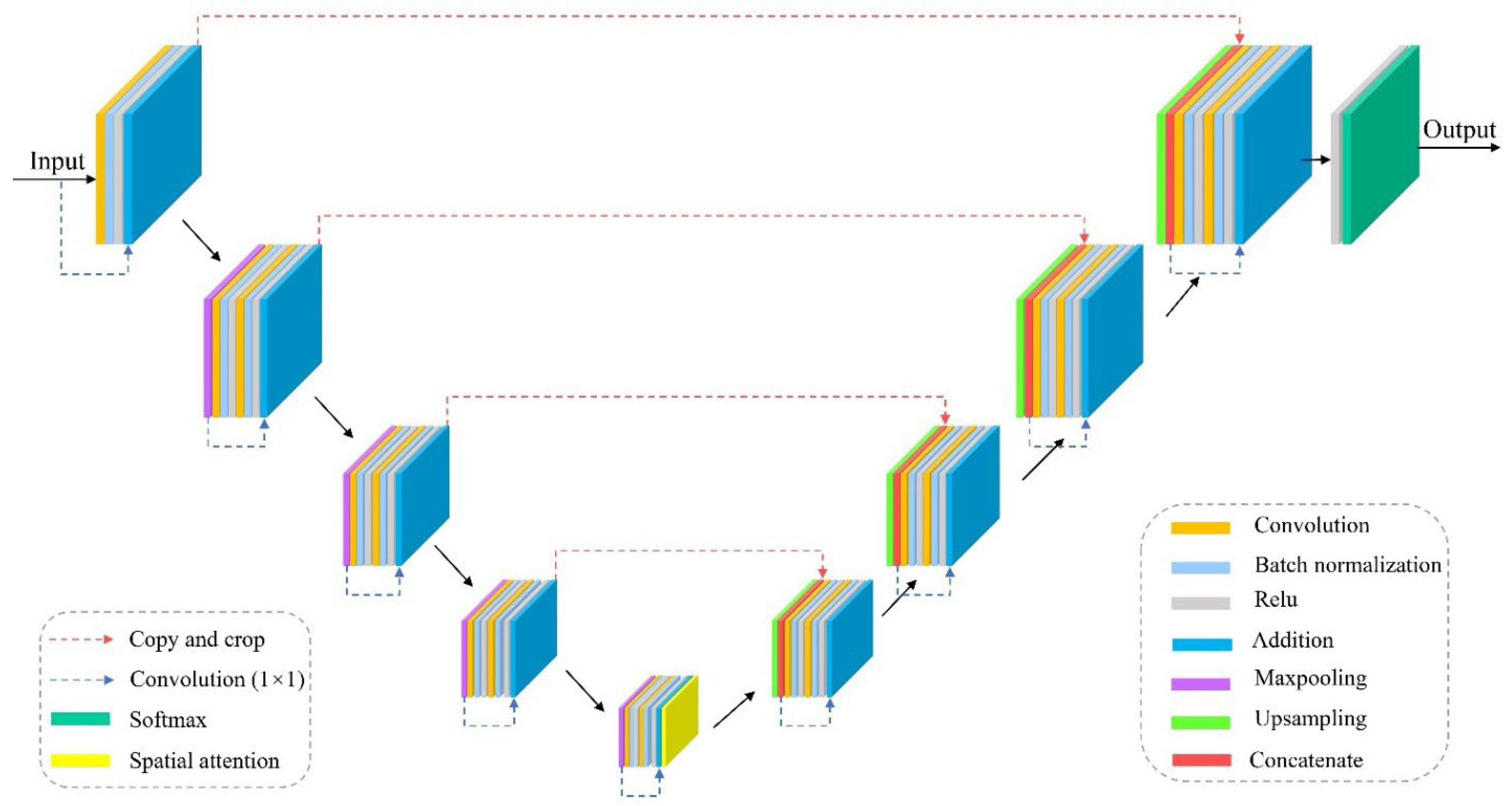
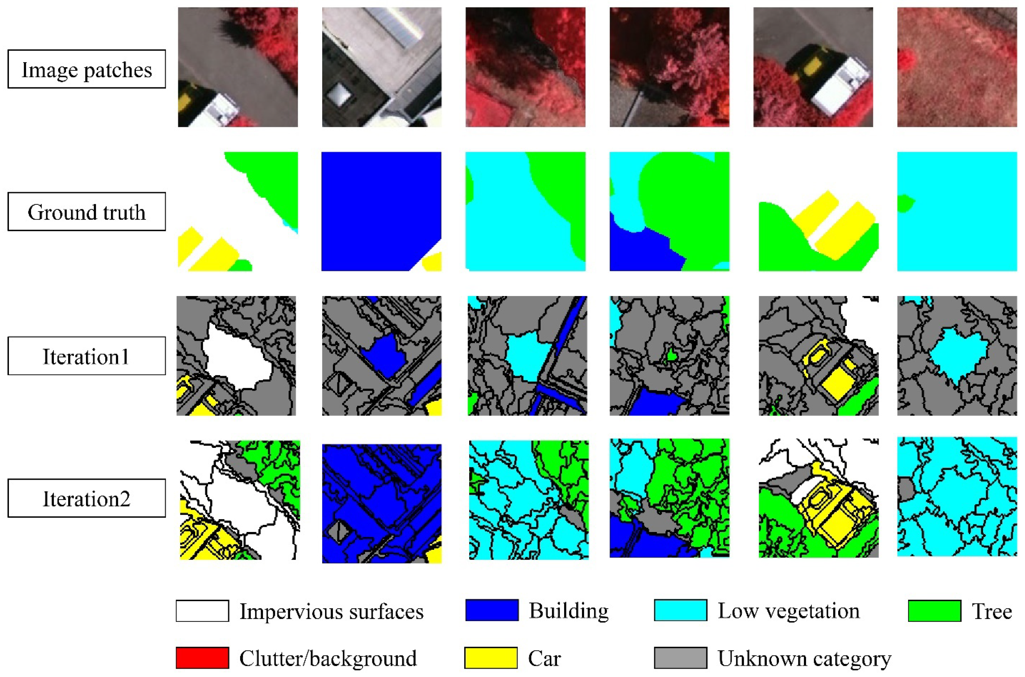
Table 1.
Image segmentation parameters and segmentation results.
| Image | Scale | Color/Shape | Smoothness/Compactness | No. of Objects | Segmentation Accuracy |
|---|---|---|---|---|---|
| V1 | 30 | 0.8/0.2 | 0.2/0.8 | 11,046 | 93.95% |
| P2 | 50 | 0.8/0.2 | 0.2/0.8 | 23,219 | 93.40% |
Table 2.
The number of sample points of each type in the two images.
| Image | Split | IS | B | LV | T | C | CB | Total |
|---|---|---|---|---|---|---|---|---|
| V1 | Train | 106 | 106 | 109 | 109 | 80 | - | 510 |
| Test | 1,414,711 | 1,314,977 | 1,014,404 | 1,129,816 | 82,424 | 4,956,332 | ||
| P2 | Train | 205 | 205 | 205 | 205 | 102 | 168 | 1090 |
| Test | 9,798,155 | 9,560,273 | 7,476,295 | 6,359,631 | 694,709 | 2,109,847 | 35,998,910 |
Note: “-” indicates that the category CB does not exist.
Table 3.
Classification accuracy comparison of the five methods for image V1.
| Model | Best Scale | OA (%) | MF1 (%) | Kappa | MCC | IS (%) | B (%) | LV (%) | T (%) | C (%) |
|---|---|---|---|---|---|---|---|---|---|---|
| OCNN | 64 | 78.33 | 71.09 | 0.7148 | 0.7153 | 78.47 | 84.30 | 65.54 | 83.15 | 71.90 |
| 2OCNN | 32/112 | 80.29 | 73.86 | 0.7403 | 0.7416 | 78.55 | 89.71 | 62.43 | 87.57 | 80.05 |
| OS-UNet | 112 | 85.97 | 81.42 | 0.8143 | 0.8147 | 86.92 | 95.10 | 73.77 | 85.48 | 80.95 |
| OS-ARU1 | 112 | 85.69 | 81.67 | 0.8106 | 0.8108 | 87.17 | 94.76 | 74.45 | 83.61 | 82.76 |
| OS-ARU | 112 | 87.83 | 84.63 | 0.8388 | 0.8389 | 90.30 | 96.32 | 77.52 | 84.40 | 84.06 |
Table 4.
Classification accuracy comparison of the five methods for image P2.
| Model | Best Scale | OA (%) | MF1 (%) | Kappa | MCC | IS (%) | B (%) | LV (%) | T (%) | C (%) | CB (%) |
|---|---|---|---|---|---|---|---|---|---|---|---|
| OCNN | 112 | 78.05 | 72.91 | 0.7198 | 0.7211 | 78.71 | 90.35 | 78.28 | 60.70 | 79.12 | 70.46 |
| 2OCNN | 64/160 | 79.76 | 75.03 | 0.7412 | 0.7419 | 80.50 | 92.67 | 76.78 | 64.97 | 85.64 | 71.11 |
| OS-UNet | 160 | 85.11 | 82.25 | 0.8088 | 0.8091 | 84.13 | 96.52 | 83.55 | 73.84 | 88.36 | 76.33 |
| OS-ARU1 | 160 | 83.68 | 79.59 | 0.7905 | 0.7913 | 85.01 | 94.54 | 84.43 | 67.95 | 82.51 | 73.42 |
| OS-ARU | 160 | 86.71 | 83.90 | 0.8292 | 0.8296 | 86.10 | 97.14 | 87.11 | 73.99 | 86.61 | 79.23 |
Table 5.
The impact of different input scales on the accuracy of OS-ARU.
| Image | 80 | 96 | 112 | 128 | 144 | 160 | 176 | 192 |
|---|---|---|---|---|---|---|---|---|
| V1 (100%) | 85.81 | 86.62 | 87.83 | 87.44 | 87.36 | 87.11 | 87.20 | 87.02 |
| P2 (100%) | 83.15 | 84.19 | 85.32 | 85.59 | 86.27 | 86.71 | 86.33 | 86.21 |
Table 6.
Model complexity comparison.
| Model | OCNN | 2OCNN | OS-U | OS-ARU | ||||
|---|---|---|---|---|---|---|---|---|
| Image | V1 | P2 | V1 | P2 | V1 | P2 | V1 | P2 |
| Parameters (MB) | 7 | 11 | 16 | 24 | 8 | 8 | 8 | 8 |
| Training time (s) | 56 | 193 | 145 | 428 | 386 | 1208 | 505 | 1577 |
| Prediction time (s) | 68 | 156 | 269 | 582 | 300 | 640 | 400 | 856 |
| Total runtime (s) | 124 | 349 | 414 | 1010 | 686 | 1848 | 905 | 2433 |
Table 7.
Module ablation experiments on OS-ARU for two images.
| Model | Image | OA (%) | MF1 (%) | Kappa | MCC | IS (%) | B (%) | LV (%) | T (%) | C (%) | CB (%) |
|---|---|---|---|---|---|---|---|---|---|---|---|
| OS-AU | V1 | 86.67 | 82.43 | 0.8236 | 0.8238 | 87.74 | 96.40 | 74.95 | 84.83 | 82.77 | - |
| OS-RU | V1 | 86.91 | 82.64 | 0.8265 | 0.8268 | 88.93 | 96.86 | 74.70 | 84.30 | 79.54 | - |
| OS-ARU | V1 | 87.83 | 84.63 | 0.8388 | 0.8389 | 90.30 | 96.32 | 77.52 | 84.40 | 84.06 | - |
| OS-AU | P2 | 85.39 | 82.47 | 0.8124 | 0.8128 | 85.29 | 96.05 | 84.88 | 72.74 | 87.03 | 77.02 |
| OS-RU | P2 | 86.46 | 83.36 | 0.8260 | 0.8263 | 85.63 | 96.78 | 86.35 | 75.14 | 86.22 | 78.11 |
| OS-ARU | P2 | 86.71 | 83.90 | 0.8292 | 0.8296 | 86.10 | 97.14 | 87.11 | 73.99 | 86.61 | 79.23 |
Note: “-” indicates that the category CB does not exist.
Table 8.
Comparison of the impact of DSL on model performance.
| Model | Image | OA (%) | MF1 (%) | Kappa | MCC | IS (%) | B (%) | LV (%) | T (%) | C (%) | CB (%) |
|---|---|---|---|---|---|---|---|---|---|---|---|
| FD-ARU | V1 | 88.63 | 76.62 | 0.8460 | 0.8461 | 92.87 | 96.97 | 73.22 | 85.09 | 32.47 | - |
| OS-ARU | V1 | 87.45 | 78.01 | 0.8297 | 0.8302 | 94.45 | 97.64 | 67.83 | 80.73 | 47.85 | - |
| FD-ARU | P2 | 88.21 | 80.45 | 0.8416 | 0.8417 | 89.35 | 97.31 | 86.16 | 74.35 | 82.46 | 51.25 |
| OS-ARU | P2 | 86.74 | 78.29 | 0.8220 | 0.8224 | 86.30 | 97.77 | 86.75 | 66.82 | 82.40 | 55.61 |
Note: “-” indicates that the category CB does not exist.
Disclaimer/Publisher’s Note: The statements, opinions and data contained in all publications are solely those of the individual author(s) and contributor(s) and not of MDPI and/or the editor(s). MDPI and/or the editor(s) disclaim responsibility for any injury to people or property resulting from any ideas, methods, instructions or products referred to in the content. |
© 2024 by the authors. Licensee MDPI, Basel, Switzerland. This article is an open access article distributed under the terms and conditions of the Creative Commons Attribution (CC BY) license (https://creativecommons.org/licenses/by/4.0/).
Share and Cite
MDPI and ACS Style
Lu, Y.; Li, H.; Zhang, C.; Zhang, S. Object-Based Semi-Supervised Spatial Attention Residual UNet for Urban High-Resolution Remote Sensing Image Classification. Remote Sens. 2024, 16, 1444. https://doi.org/10.3390/rs16081444
AMA Style
Lu Y, Li H, Zhang C, Zhang S. Object-Based Semi-Supervised Spatial Attention Residual UNet for Urban High-Resolution Remote Sensing Image Classification. Remote Sensing. 2024; 16(8):1444. https://doi.org/10.3390/rs16081444
Chicago/Turabian StyleLu, Yuanbing, Huapeng Li, Ce Zhang, and Shuqing Zhang. 2024. "Object-Based Semi-Supervised Spatial Attention Residual UNet for Urban High-Resolution Remote Sensing Image Classification" Remote Sensing 16, no. 8: 1444. https://doi.org/10.3390/rs16081444
Note that from the first issue of 2016, this journal uses article numbers instead of page numbers. See further details here.