Canopy-Level Spectral Variation and Classification of Diverse Crop Species with Fine Spatial Resolution Imaging Spectroscopy

Abstract

With the increasing availability and volume of remote sensing data, imaging spectroscopy is an expanding tool for agricultural studies. One of the fundamental applications in agricultural research is crop mapping and classification. Previous studies have mostly focused at local to regional scales, and classifications were usually performed for a limited number of crop types. Leveraging fine spatial resolution (60 cm) imaging spectroscopy data collected by the Global Airborne Observatory (GAO), we investigated canopy-level spectral variations in 16 crop species from different agricultural regions in the U.S. Inter-specific differences were quantified through principal component analysis (PCA) of crop spectra and their Euclidean distances in the PC space. We also classified the crop species using support vector machines (SVM), demonstrating high classification accuracy with a test kappa of 0.97. A separate test with an independent dataset also returned high accuracy (kappa = 0.95). Classification using full reflectance spectral data (320 bands) and selected optimal wavebands from the literature resulted in similar classification accuracies. We demonstrated that classification involving diverse crop species is achievable, and we encourage further testing based on moderate spatial resolution imaging spectrometer data.

1. Introduction

In 2015, the United Nations General Assembly identified 17 global Sustainable Development Goals (SDGs), the second of which (i.e., SDG 2 “Zero hunger”) was to “End hunger, achieve food security and improved nutrition and promote sustainable agriculture” [1]. To achieve these goals, food production shall be increased while sustainable practices and management of agricultural lands should be reinforced [2]. Remote sensing has long been recognized as a powerful tool for assisting sustainable agriculture because of the need for spatially consistent data across large scales, and remotely sensed information has been used for numerous agricultural applications, including but not limited to phenotyping, land-use monitoring, crop-yield forecasting, precision agriculture, and preserving agroecosystem services [3].

One of the basic and heavily studied applications of remote sensing in agriculture focuses on the mapping and classification of different crop species [4,5,6]. Accurate and timely crop mapping is a prerequisite for crop yield estimation, thus crucial for global food security and socioeconomic stability [7]. Traditional multispectral data, such as those collected by Landsat, MODIS, and Sentinel-2, have been widely used to distinguish different types of land cover and use, for example, green vegetation, soil, impervious surfaces, water, etc. [8,9,10]. However, with limited spectral bands and coarse spectral resolutions, classifying crop types with such data is challenging and usually requires additional information input, such as incorporating multi-temporal data from the entire growing season [11,12].

According to the spectral diversity theory, the variability in spectral reflectance data from plant communities can correspond to plant taxonomic, phylogenetic, and functional diversity [13,14]. In addition, different crop growth status, canopy structures, pigment concentrations, and leaf water contents all affect the reflectance spectrum of crops, thus providing the theoretical foundations for differentiation [15,16,17]. Imaging spectroscopy, or hyperspectral remote sensing, can provide a promising tool for crop classification [18,19]. Instead of using a few broad bands, this technique provides spectral information in hundreds of continuous channels, and thus can be sensitive to the subtle differences between different crop species and conditions [20].

Several studies have investigated crop classification using imaging spectroscopy data collected from various platforms, including field spectroradiometers, unmanned aerial vehicles (UAVs), and airplanes as well as satellites, and moderate to excellent classification accuracies have been achieved [21,22,23,24,25]. However, the study areas were usually confined to a single site, and the number of crop types examined was usually limited. By leveraging data collected by the Global Airborne Observatory (GAO, formerly known as Carnegie Airborne Observatory [26]) and corresponding ground reference information, we examined canopy-level spectral variations in 16 different crop species from different agricultural regions in the contiguous U.S. We also explored the classification of different crop species and examined if such a classification scheme with fine spatial resolution imaging spectroscopy data was achievable.

2. Materials and Methods

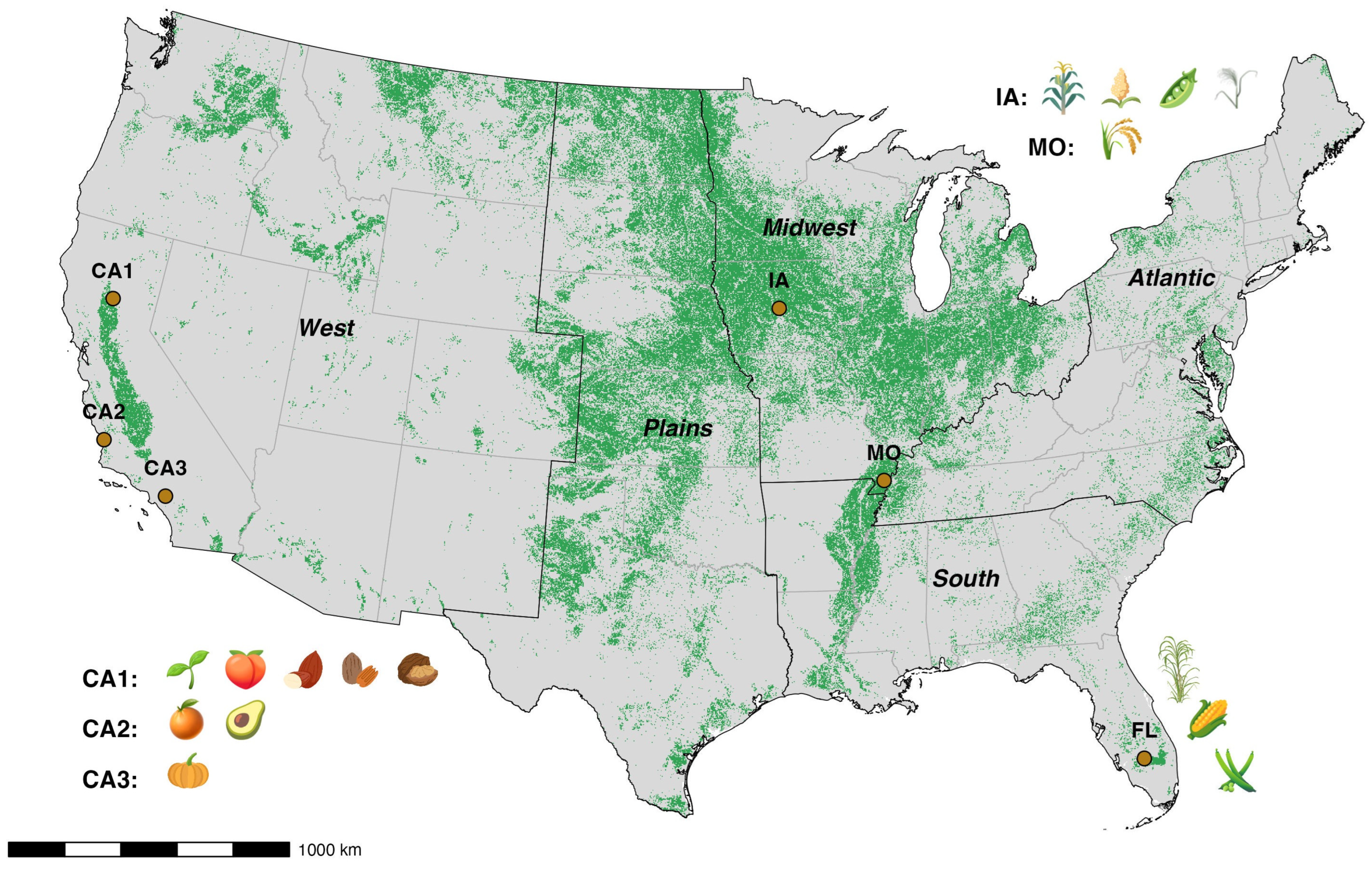
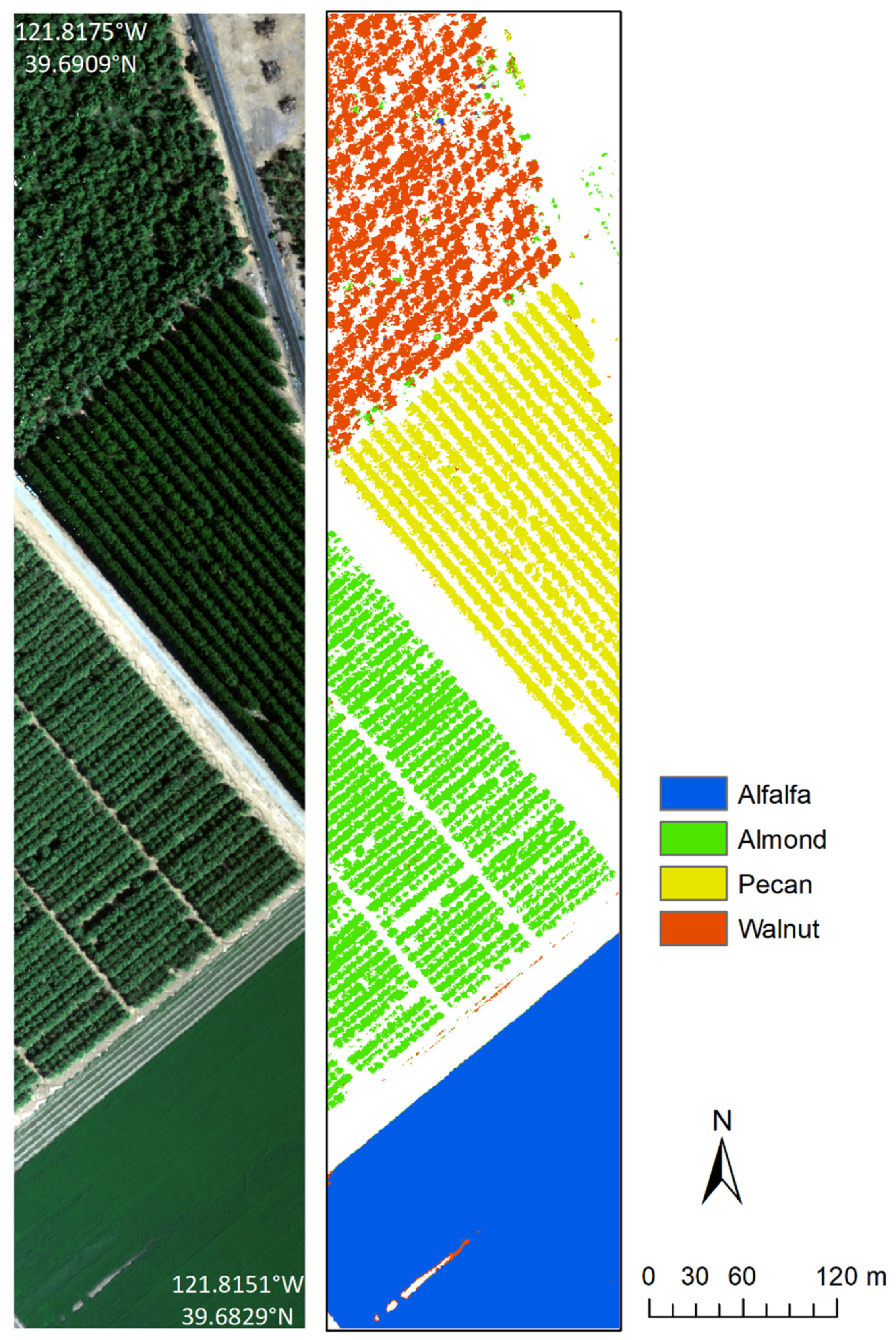
2.1. Study Sites

We analyzed image data from six sites in the contiguous U.S., located in three of the five major U.S. farming regions [27,28], including the South, the Midwest, and the West (Figure 1;

Table 1. Summary table of crop species, number of polygons, and available spectra sample sizes after spectral filtering.

Site	Crop	Polygons	Reflectance Spectra
CA1	Alfalfa	2	17,384
	Almond	4	11,573
	Peach	2	6810
	Pecan	2	10,267
	Walnut	3	10,214
CA2	Avocado	2	8931
	Orange	2	6361
	Pumpkin	2	9052
FL	Green Bean	3	12,684
	Sugarcane	4	11,433
	Sweet Corn	2	17,433
IA	Grain Corn	2	13,624
	Miscanthus	2	12,034
	Sorghum	2	20,253
	Soybean	2	17,281
MO	Rice	2	13,224

). The Florida (FL) site incorporated selected croplands of the Rouge River Farm in Hendry County, Florida. Cultivated crops include sugarcane, sweet corn, green bean, etc. The Missouri (MO) site encompassed the research fields around the Fisher Delta Research, Extension, and Education Center in Portageville, Missouri. Crops included species of major importance to the region, namely, rice, cotton, peanuts, soybeans, etc. The Iowa (IA) site was a sustainable advanced bioeconomy research farm in Boone County, Iowa, close to Iowa State University campus. In addition to the energy crop Miscanthus, soybean, sorghum, and grain corn were also planted in 2022. The northmost California (CA1) site was a research farm located five miles south of California State University, Chico campus. Main crops investigated included orchard species such as almond, peach, pecan, and walnut, as well as alfalfa. A second California (CA2) site was within the Cal Poly Organic Farm, located on Cal Poly San Luis Obispo campus. Citrus, olive, avocado, and pomegranate were the major crops. The third California (CA3) site was the Cal Poly Pomona campus farm, growing melon, orange, pumpkin, and other vegetables.

2.2. Data Collection and Processing

Image data covering the visible to shortwave infrared (VSWIR) wavelength range were acquired by the GAO. The VSWIR data spanned 428 bands between 350 nm and 2490 nm with a full-width, half-maximum of about 5 nm. With flight elevation around 600 m above ground, the orthorectified imagery had a spatial resolution of about 0.6 m. Alongside VSWIR data, Light detection and ranging (LiDAR) data were also collected to help ortho-georeference the images, as well as to produce digital terrain and surface models. The raw VSWIR data were first processed to radiance using current spectral calibration, and then to surface reflectance (values between 0 and 1) through atmospheric correction with ACORN v6.0 (Atmospheric CORrection Now; AIG LLC; Boulder, CO, USA). We refer to Asner et al. [29] for more details on VSWIR data preprocessing and surface reflectance retrieval. We removed wavelengths known to have low signal-to-noise ratio, resulting in 320 bands spanning the wavelength regions 420–1330, 1500–1775, and 2030–2445 nm for further analysis.

A suite of spectral filters was applied to remove non-vegetation and shaded pixels [28]. First, we applied a narrow band Normalized Difference Vegetation Index (NDVI; near-infrared: 860 nm; red: 650 nm) to remove non-vegetation pixels, where all pixels with an NDVI value lower than 0.7 were excluded [30]. Then, we removed all pixels dominated by shadow using a brightness filter and included only pixels with a reflectance value higher than 25% at 1070 nm wavelength [30]. In addition to original reflectance, we applied brightness normalization to further dampen the potential contribution of plant biophysical conditions [31].

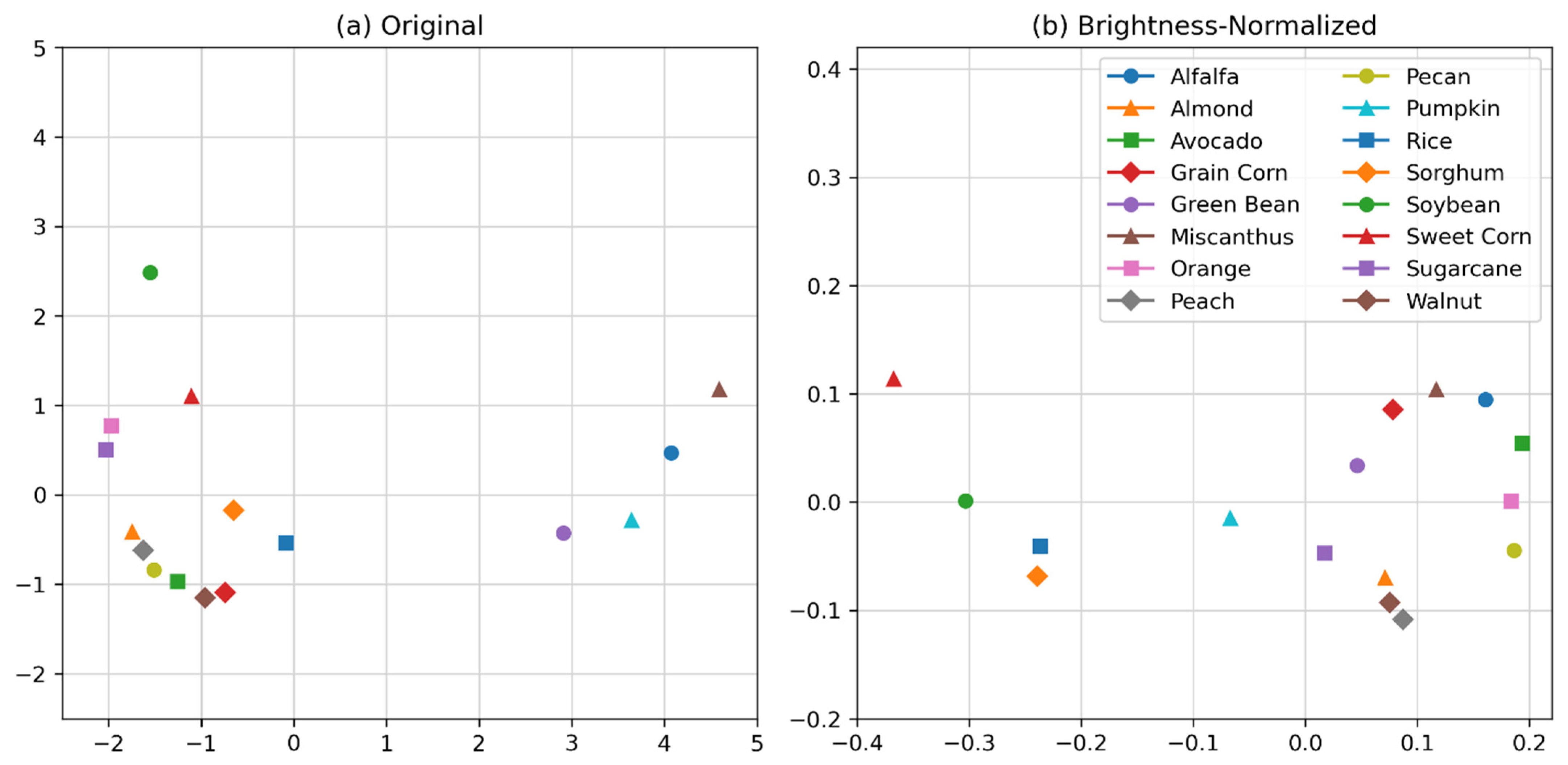
2.3. Spectral Variation

We chose 16 crop species with sufficient sample size (i.e., more than 6000 pixels) for investigation, and for each crop species, at least two polygons were identified in the VSWIR data (Table 1). After spectral filtering, the available number of pixels for each species varied from more than 6000 to just above 20,000. We examined the mean spectra of both original and brightness-normalized reflectance data. We calculated the coefficient of variation (CV; standard deviation divided by mean) for each band of the brightness-normalized spectra, as a proxy of intra-specific variations in vegetation conditions [30,32].

Next, to investigate the inter-specific spectral variations in different crop species, we applied principal component analysis (PCA) to the original reflectance spectra that passed the filtering. Based on the smallest number of pixels of all crops (i.e., 6361 for orange; Table 1), we randomly selected 6000 pixels from each species. This step was to guarantee the equal contribution of all crop species to the PCA, as this method is sensitive to relative group size. In total, 96,000 (6000 × 16) pixels were used in the PCA. The above PCA calculations were replicated for the brightness-normalized spectra as well. Moreover, to compare how crop species separate from each other, we calculated the Euclidean distance between species centroids in PC space (first 16 PC bands [30], which explained more than 99.9% of the variance) as an estimation of species similarity. We projected the 16-dimensional Euclidean distance onto a 2-dimensional plot using the multi-dimensional scaling function provided by the scikit-learn package (version 1.0.2) [33] in Python (version 3.6.9).

2.4. Classification Strategies

We used the support vector machine (SVM) classification algorithm to classify the diverse crop types due to its effectiveness and handiness identified by previous studies [34,35,36,37]. The SVM parameters included a radial basis function (i.e., kernel = ‘rbf’) and default gamma (i.e., ‘scale’). To examine the balance between classification accuracy and complexity of the decision surface, we tested a suite of different cost parameter C values (i.e., 1, 10, 100, and 1000). The classification was performed in Python (version 3.6.9) using the scikit-learn package (version 1.0.2) [33]. Since both plant biophysical and biochemical conditions can contribute to the spectral differences between different crop species, we incorporated the original reflectance data for the classification.

2.4.1. Training and Test Data

Given the number of polygons and the abundance of available pixels for each species after spectral filtering (Table 1), we randomly picked one polygon and selected 3000 pixels as potential training data for classification, respectively. Another 3000 pixels were randomly selected from the remaining polygon(s) as test data. To examine the effect of training data size on classification accuracy, we tested a suite of different training sample size values (i.e., 50, 100, 200, 500, 1000, 2000, and 3000) while keeping the validation sample size constant (i.e., 3000).

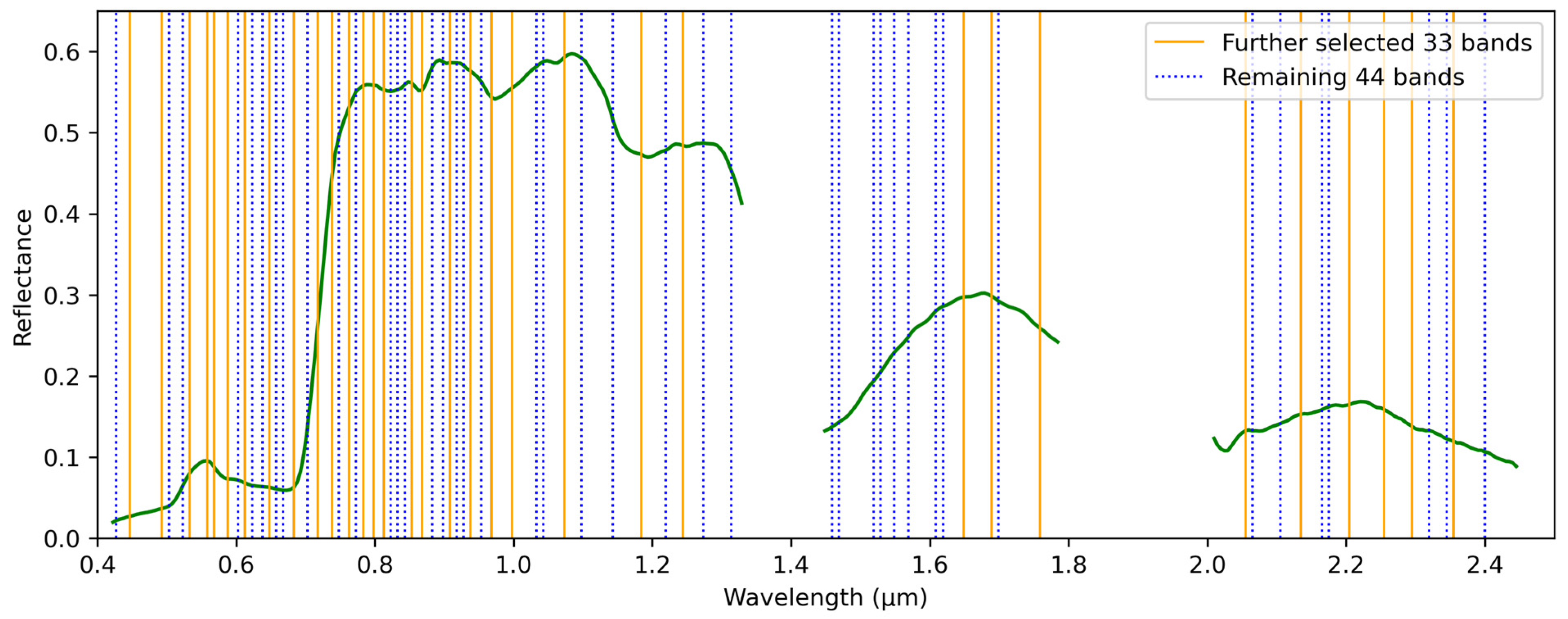
2.4.2. Full Spectrum vs. Selected Bands

Classification was first performed using full spectrum data (i.e., 320 bands). To address the potential issue of the Hughes phenomenon [38], in which the increased dimensionality of data may decrease classification accuracy, we also applied the classification using subsets of the 320 available bands. Several studies have identified optimal wavelengths that are useful for crop classification [22,39,40,41], from which we compiled all optimal wavelengths and identified relevant GAO bands (Figure 2). In total, 77 bands were selected by at least one of the studies mentioned above, and 33 bands were selected by at least two. Detailed information on selected wavelengths and corresponding GAO bands can be found in

Table A2. Selected 77 GAO bands and wavelength (in nm) for classification. Italic records indicate further selected 33 bands.

Band	Wavelength	Band	Wavelength	Band	Wavelength	Band	Wavelength
17	427.4	81	747.9	138	1033.3	269	1689.3
21	447.4	84	762.9	140	1043.3	271	1699.3
30	492.5	86	772.9	146	1073.4	283	1759.4
32	502.5	88	783.0	151	1098.4	342	2054.9
36	522.6	91	798.0	160	1143.5	344	2064.9
38	532.6	94	813.0	162	1153.5	352	2104.9
43	557.6	96	823.0	168	1183.6	358	2135.0
45	567.6	98	833.0	175	1218.6	364	2165.0
49	587.7	100	843.0	180	1243.6	366	2175.0
52	602.7	102	853.0	186	1273.7	372	2205.1
54	612.7	105	868.1	194	1313.7	382	2255.1
56	622.7	108	883.1	223	1459.0	390	2295.2
59	637.7	111	898.1	225	1469.0	395	2320.3
61	647.7	113	908.1	235	1519.1	400	2345.3
63	657.8	115	918.2	237	1529.1	402	2355.3
65	667.8	117	928.2	241	1549.1	411	2400.4
68	682.8	119	938.2	245	1569.1	417	2430.4
72	702.8	122	953.2	253	1609.2
75	717.8	125	968.2	255	1619.2
79	737.9	131	998.3	261	1649.2

.

2.4.3. Accuracy Assessment

For each combination of classification configuration (i.e., C ∈ [1, 10, 100, 1000] and training sample size ∈ [50, 100, 200, 500, 1000, 2000, 3000]), we conducted the classification 50 times (i.e., 50 iterations). For each iteration, the overall accuracy, kappa, error matrix, and species-specific user’s and producer’s accuracies (UA, PA) were calculated. The final statistics were averaged from the 50 iterations. The above procedure was applied for all classification attempts in this paper. Classification was first performed within individual sites. Due to the number of species at each site and geographical proximity, Sites CA2 and CA3, as well as Sites IA and MO, were merged, respectively. After that, a pooled classification incorporating all crop species across all sites was also examined.

Given data availability, the training and test data of each crop species described in Section 2.4.1 were all from the same site. In addition, we incorporated a separate test dataset with GAO imagery of grain corn collected from the MO site, which was not used for the SVM model training. We applied the same spectral filters, randomly selected 3000 test pixels, and applied the classifier trained from the pooled training data. If the test pixel was classified as any of the 15 species other than “Grain Corn”, it would be considered a misclassification. The same classification parameter combinations (i.e., training size of each species ∈ [50, 100, 200, 500, 1000, 2000, 3000] and C ∈ [1, 10, 100, 1000]) were permutated and tested. Classification accuracy was averaged from 50 iterations.

3. Results

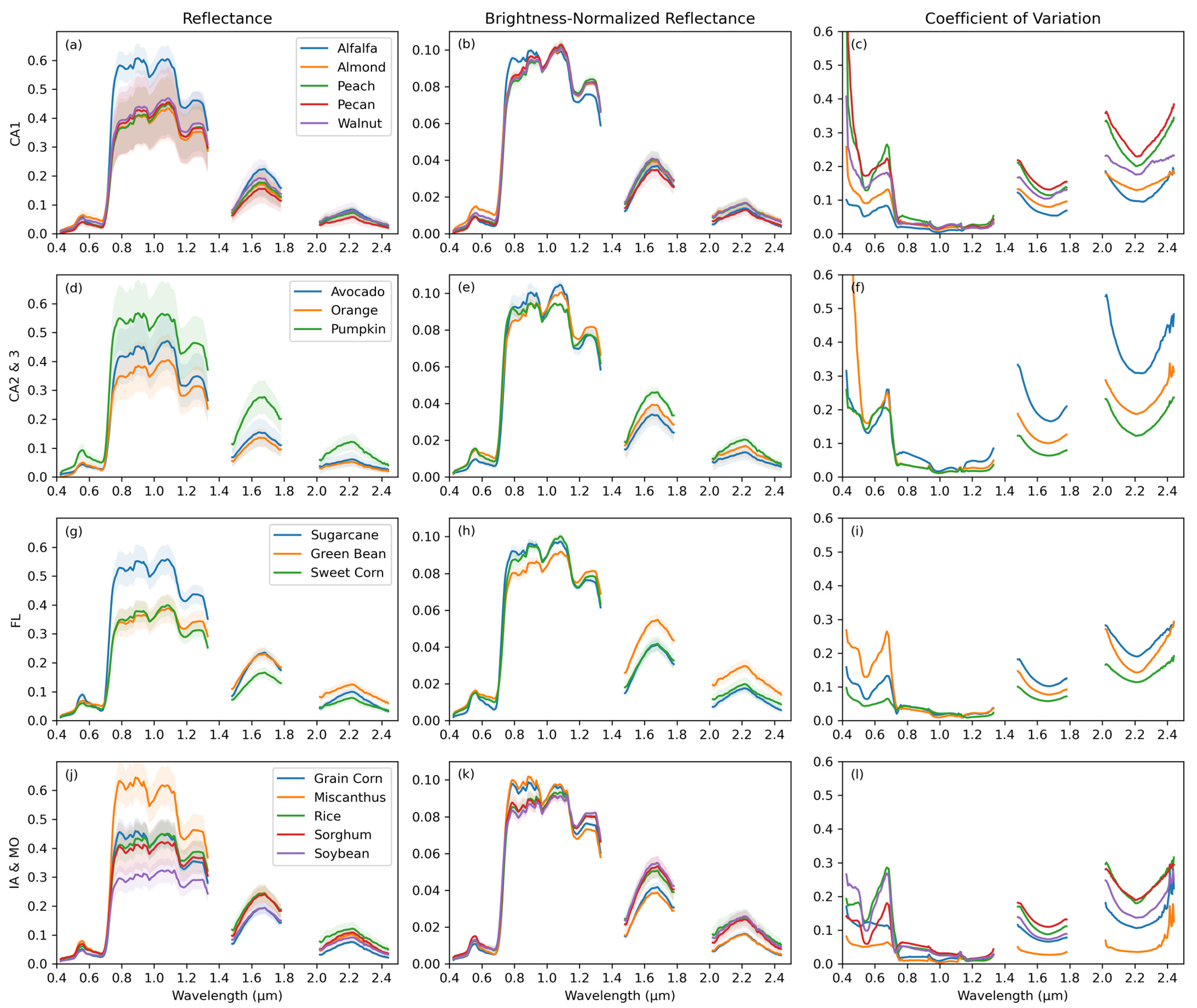
3.1. Crop Spectra and Spectral Variation

We compared the average and standard deviation of reflectance spectra of each crop species using all available pixels after spectral filtering (Figure 3 and Figure A1). In general, of all crops in our dataset, Miscanthus had the highest reflectance in the near-infrared (NIR), whereas soybean had the lowest values. In addition, alfalfa, pumpkin, and sugarcane were much brighter than the remaining species in the NIR. Moreover, all tree species (i.e., almond, peach, pecan, walnut, avocado, and orange) and pumpkin showed a much higher standard deviation in NIR than the other herbaceous species (Figure A1). In the 1500–1800 nm short-wave infrared wavelength (i.e., SWIR I), pumpkin had the highest reflectance and orange had the lowest. No species stood out in the visible (400–700 nm) or SWIR II (2050–2400 nm) wavelengths.

In the comparison of different spectra, brightness normalization can highlight distinct spectral shapes while minimizing overall brightness differences [31]. After brightness normalization, crop reflectance variability was reduced within the water absorption wavelength around 1200 nm (Figure 3 and Figure A1). In general, comparing all crop species, normalized reflectance converged in the NIR and expanded in visible red (600–700 nm) and the SWIR II portion of the spectrum. Sweet corn had the highest reflectance in SWIR II after brightness normalization, whereas no species stood out in other wavelengths.

The CV of the spectra suggested that intra-specific variations were responsive to crop functional types (i.e., tree or herbaceous; Figure 3c). In the SWIR region, tree species generally had a larger CV than herbaceous ones. The CV of avocado was the largest, followed by pecan and peach. On the other hand, Miscanthus had the lowest CV, suggesting relatively homogenous crop conditions. In visible blue (400–500 nm), orange, pecan, and peach had larger CVs than the other species, whereas in visible red (600–700 nm), pumpkin showed a slightly higher CV than the other crops.

For original reflectance, the Euclidean distances between crop centroids in PC space were dominated by overall spectral brightness, and the brightest species (i.e., Miscanthus) was furthest from 12 of the 16 crops (Figure 4a and

Table A3. Euclidean distance between the crop centroids in principal component (PC) space. Distances were calculated using original reflectance PCs 1–16 (bottom triangle) and brightness-normalized reflectance PCs 1–16 (top triangle). Orange cells indicate the most distant species of each species.

	Alfalfa	Almond	Avocado	Grain Corn	Green Bean	Miscanthus	Orange	Peach	Pecan	Pumpkin	Rice	Sorghum	Soybean	Sweet Corn	Sugarcane	Walnut
Alfalfa	0	0.084	0.042	0.044	0.062	0.040	0.051	0.089	0.067	0.101	0.159	0.156	0.181	0.213	0.085	0.081
Almond	1.83	0	0.079	0.080	0.057	0.092	0.056	0.048	0.063	0.075	0.114	0.115	0.134	0.158	0.037	0.028
Avocado	1.61	0.40	0	0.065	0.080	0.057	0.039	0.081	0.054	0.116	0.164	0.167	0.190	0.217	0.083	0.075
Grain Corn	1.46	0.49	0.33	0	0.055	0.031	0.075	0.083	0.084	0.075	0.125	0.121	0.148	0.180	0.067	0.073
Green Bean	0.51	1.43	1.28	1.10	0	0.063	0.066	0.083	0.087	0.048	0.117	0.110	0.134	0.165	0.049	0.064
Miscanthus	0.35	2.08	1.86	1.69	0.72	0	0.075	0.102	0.093	0.089	0.145	0.143	0.170	0.199	0.080	0.090
Orange	2.18	0.45	0.60	0.79	1.82	2.44	0	0.068	0.039	0.105	0.157	0.158	0.179	0.207	0.074	0.058
Peach	1.76	0.23	0.37	0.45	1.39	2.01	0.55	0	0.049	0.098	0.115	0.120	0.136	0.164	0.060	0.025
Pecan	1.68	0.30	0.25	0.42	1.34	1.95	0.54	0.21	0	0.121	0.158	0.160	0.179	0.208	0.084	0.053
Pumpkin	0.61	1.73	1.61	1.41	0.40	0.64	2.13	1.68	1.67	0	0.080	0.070	0.095	0.126	0.057	0.080
Rice	1.54	0.71	0.81	0.61	1.10	1.72	1.11	0.66	0.80	1.26	0	0.033	0.039	0.059	0.092	0.109
Sorghum	1.70	0.55	0.72	0.53	1.26	1.90	0.91	0.54	0.69	1.45	0.28	0	0.031	0.069	0.095	0.111
Soybean	2.67	0.92	1.21	1.25	2.25	2.89	0.76	0.99	1.13	2.48	1.27	1.04	0	0.051	0.117	0.129
Sweet Corn	2.17	0.68	0.98	0.91	1.72	2.36	0.88	0.73	0.92	1.90	0.66	0.50	0.69	0	0.138	0.158
Sugarcane	2.15	0.37	0.63	0.73	1.76	2.39	0.29	0.48	0.58	2.04	0.92	0.71	0.61	0.61	0	0.044
Walnut	1.51	0.36	0.39	0.34	1.12	1.76	0.77	0.28	0.32	1.41	0.51	0.47	1.21	0.81	0.70	0

). As the darkest species, soybean was furthest from the four remaining crops (i.e., alfalfa, green bean, Miscanthus, and pumpkin). On the other hand, brightness normalization dampened the contribution from biophysical conditions to crop spectra and highlighted the biochemical variability in crop canopy reflectance. After brightness normalization, sweet corn was furthest from 12 of the 16 crops, and avocado was furthest from the 4 remaining crops (i.e., rice, sorghum, soybean, and sweet corn; Figure 4b and Table A3). For original reflectance data, the centroids of most tree species (i.e., almond, peach, pecan, walnut, and avocado) were close to each other in the PC space. Whereas for brightness normalized reflectance data, almond, walnut, and peach were still similar, but avocado and pecan were further away. Another group of crops that distanced themselves from each other after normalization was orange, sugarcane, and sweet corn.

3.2. Classification Results

3.2.1. Training Sample Size and Cost Parameter

The cost parameter C in SVM is a hyperparameter defining the trade-off between training error and separating margin size, where larger C values will result in fewer misclassifications but a smaller margin [34]. High C values can potentially result in overfitting to the training data and drastically lower test classification accuracy if the test data are spectrally different from the training data. Within the test range of C values in our investigation, training and test kappa values were all similar (

Table 2. Training/test kappa values of pooled classification (i.e., including all 16 crop species) for different training data size (i.e., “Spectra” of each crop species) and cost parameter (C) combinations using full spectrum GAO data. All values were rounded to two decimal places.

Spectra	C = 1	C = 10	C = 100	C = 1000
50	0.39/0.39	0.80/0.76	0.97/0.95	1.00/0.97
100	0.54/0.53	0.85/0.85	0.98/0.97	1.00/0.99
200	0.64/0.64	0.91/0.91	0.99/0.99	1.00/1.00
500	0.75/0.75	0.96/0.95	1.00/0.99	1.00/1.00
1000	0.86/0.86	0.98/0.97	1.00/1.00	1.00/1.00
2000	0.91/0.91	0.99/0.99	1.00/1.00	1.00/1.00
3000	0.94/0.94	0.99/0.99	1.00/1.00	1.00/1.00

). However, C could greatly affect classification accuracies, especially when the training sample size was small. When a default C value (i.e., C = 1) was applied, about 2000 training spectra were needed to achieve a test kappa value higher than 0.9. On the other hand, when C was set to be 100 or higher, only 50 training pixels were needed to produce similar classification accuracies. When C values were high, both training and test kappa values could easily surpass 0.95.

According to the permutation tests, the test accuracy on the separate grain corn dataset peaked at 0.95 when 1000 training pixels were selected from each crop and C = 10. The inclusion of more training pixels did not further increase the accuracy, whereas increased C decreased the accuracy. Thus, for the rest of this paper, we will discuss the classification results of 1000 training pixels per crop and C = 10.

3.2.2. Different Classification Strategies

We explored the classification of limited species within individual sites and achieved excellent kappa values (i.e., 0.96–0.99) [42] for all sites (

Table 3. Test kappa values of individual sites as well as cross-site pooled data (i.e., all 16 species). All values were rounded to two decimal places.

Site	Species	Full Spectrum	77 Bands	33 Bands
CA1	5	0.96	0.96	0.94
CA2 and CA3	3	0.99	0.99	0.99
FL	3	0.99	0.99	0.99
IA and MO	5	0.99	0.98	0.98
Pooled	16	0.97	0.97	0.97

). Moreover, both full spectrum and selected bands resulted in similar classification accuracies. The accuracy of Site CA1, where four of the five crop species were orchard trees, was slightly lower than the other sites. This is probably due to their less-distinct spectral features, as discussed in Section 3.1.

Illustrations of a species map separating grain corn, Miscanthus, sorghum, and soybean at Site IA are shown in Figure 5. Note that based on the classifier trained from the training dataset, all pixels that passed the spectral filters were mapped. Thus, grasses between different crop fields were classified as the crop that was most similar to them in terms of reflectance (in this case, soybean). A similar crop map separating alfalfa, almond, pecan, and walnut at Site CA1 is shown in Figure 6.

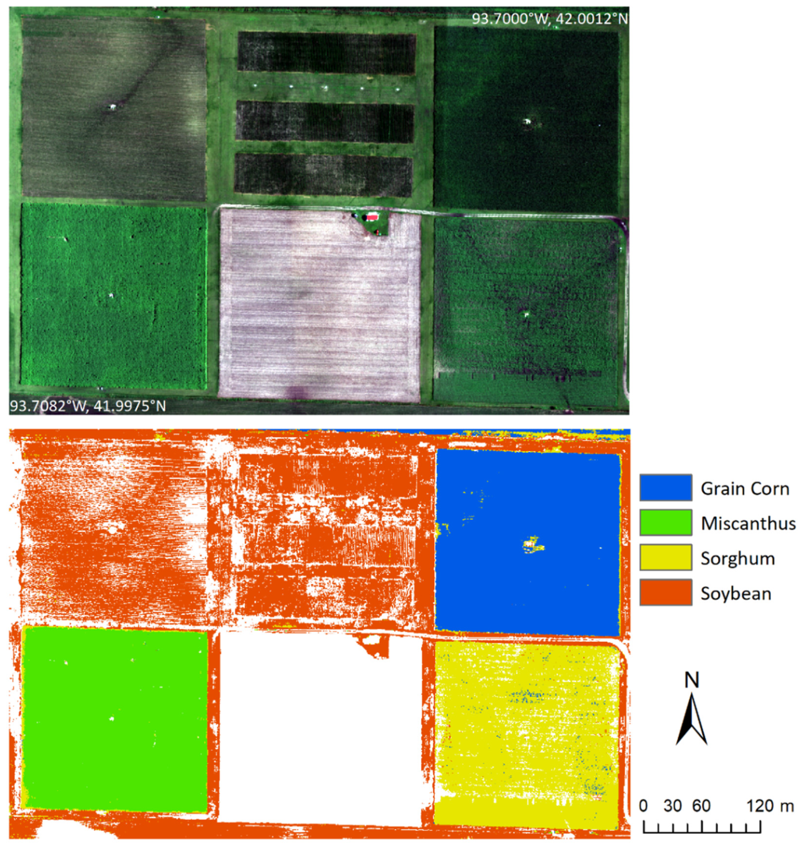
3.2.3. Pooled Classification

We performed a pooled classification for all 16 crop species across different sites and achieved high accuracy (test kappa = 0.97; Table 3). As for the individual sites, classification using the full spectrum or selected bands produced similar test kappa values and confusion matrices. Here, we report the classification results using the full spectrum data. Based on the error matrix averaged from 50 iterations, all crops but walnut achieved classification accuracies higher than 95%, with walnut at 92.66% (

Table 4. Error matrix averaged from 50 iterations of classification using full spectrum. Blank cells indicate a 0 misclassification rate. Otherwise, all values were rounded to two decimal places. Colors indicate (mis)classification percentages: Green, <1 or >95, and Yellow, 1–5 or 90–95. Note that because the results were averaged from 50 iterations, numbers in each line do not add up to 100.

	Alfalfa	Almond	Avocado	Grain Corn	Green Bean	Miscanthus	Orange	Peach	Pecan	Pumpkin	Rice	Sorghum	Soybean	Sweet Corn	Sugarcane	Walnut
Alfalfa	99.17			0.08	0.04		0.00			0.00	0.55	0.11	0.00		0.00	0.03
Almond		99.37					0.00	0.02	0.01						0.02	0.57
Avocado	0.02	0.20	96.32		0.00		0.03	1.21	0.21	0.01	0.18			0.14	0.34	1.33
Grain Corn	0.03	0.00	0.00	98.28		0.25	0.00			0.02	0.15	1.26
Green Bean	0.02	0.01			98.78	0.01	0.01	0.02	0.01	0.36	0.04		0.07	0.49	0.15	0.03
Miscanthus		0.00	0.02	1.47		98.30				0.13	0.05	0.01		0.01	0.00
Orange		0.68	0.33		0.07		97.58	0.26	0.04	0.03	0.06		0.05	0.10	0.19	0.63
Peach		0.01	0.48				0.01	97.53	0.24	0.01	0.02		0.00	0.28	0.10	1.32
Pecan		0.68	0.18				0.05	2.18	96.15		0.06		0.01	0.10	0.05	0.55
Pumpkin	0.05		0.02	0.15	0.45	0.22	0.10	0.01		97.85	0.56	0.04	0.39	0.04	0.05	0.07
Rice	0.34		0.00	0.45		0.01		0.01		0.04	98.74	0.01	0.33	0.06	0.00
Sorghum	0.20			1.65	0.00	0.00				0.03	0.05	97.45	0.61
Soybean	0.02			0.27	0.01					0.01	0.02	0.62	98.96	0.08
Sweet Corn				0.01	0.05			0.01	0.00	0.00	0.16		0.03	99.60	0.13
Sugarcane	0.03	0.20	0.10		0.26					0.01				0.42	98.98
Walnut	0.03	1.88	0.24	0.01	0.06	0.01	0.10	3.01	0.52	0.05	0.36	0.00	0.53	0.46	0.08	92.66

). For all crops, PA and UA were above 90%, and most of them were above 95% (

Table 5. Pooled classification results with producer’s (PA) and user’s (UA) % accuracies. For each crop, the “Classified As” column indicates the crop that it was most frequently misclassified as, and the “Classified” column indicates the crop that it most frequently misclassified, based on the averaged error matrix.

Crop	Site	PA	UA	Classified As	Classified
Alfalfa	CA1	99.3	99.2	Rice	Rice
Almond	CA1	96.5	99.4	Walnut	Walnut
Avocado	CA2	98.6	96.3	Walnut	Peach
Grain Corn	IA	96.1	98.3	Sorghum	Sorghum
Green Bean	FL	99.1	98.8	Sweet Corn	Pumpkin
Miscanthus	IA	99.5	98.3	Grain Corn	Grain Corn
Orange	CA2	99.7	97.6	Almond	Walnut
Peach	CA1	93.6	97.5	Walnut	Walnut
Pecan	CA1	98.9	96.2	Peach	Walnut
Pumpkin	CA3	99.3	97.8	Rice	Green Bean
Rice	MO	97.8	98.7	Grain Corn	Pumpkin
Sorghum	IA	97.9	97.5	Grain Corn	Grain Corn
Soybean	IA	98.0	99.0	Sorghum	Sorghum
Sweet Corn	FL	97.9	99.6	Rice	Green Bean
Sugarcane	FL	98.9	99.0	Sweet Corn	Avocado
Walnut	CA1	95.3	92.7	Peach	Avocado

). The only exceptions were the PA of peach and the UA of walnut, which were 93.6% and 92.7%, respectively. As for misclassification, the most frequently confused species were often within the same functional type. For example, walnut showed the lowest classification rate, and it was most frequently misclassified as peach. Euclidean distance between them also indicates they are the closest species (Table A3). Moreover, alfalfa, pumpkin, and sweet corn were most frequently misclassified as rice; almond, avocado, and peach were most frequently misclassified as walnut; Miscanthus, rice, and sorghum were most frequently misclassified as grain corn, etc.

4. Discussion

We explored the canopy-level spectral variation and classification of crop types with fine spatial resolution imaging spectroscopy data. We trained an SVM classifier with training spectra from 16 crop species and achieved an excellent test accuracy (kappa = 0.97). We also tested the classifier with a separate grain corn dataset and achieved comparable test accuracy (kappa = 0.95). Our study shows that the classification of diverse crop species using imaging spectroscopy data is achievable.

In land-cover classification using moderate spatial resolution data, one of the major challenges is dealing with mixed pixels. In the case of classifying plants, the detected spectral profile may include contributions from not only green vegetation, but also from non-photosynthetic vegetation (NPV) and substrate material [43]. The GAO data used in this work had a spatial resolution of 0.6 m; thus, most of the image pixels can be considered as “pure” from a spectral unmixing perspective. In addition, we applied NDVI and brightness filters to exclude pixels dominated by or had significant portions of NPV, soil, or shadows. These procedures ensured that the inputs to the classification were pixels representing green vegetation under desirable illumination conditions.

Imaging spectroscopy data with continuous spectral reflectance within VSWIR wavelengths provide abundant information that can be helpful in discriminating between different plant species. Whereas traditional multispectral data such as those collected by Landsat and Sentinel-2 were mostly applied for identifying general land-cover types, imaging spectroscopy data have been used to classify different plant species and even intra-species varieties [30,44]. Moreover, the uniformly high signal-to-noise ratio (SNR) of GAO data helped in modeling and accounting for atmospheric water vapor and aerosols in the spectrum, so that the retrieved surface reflectance data were of high quality and suitable for vegetation and ecosystem mapping purposes [18,26].

Another unneglectable factor attributing to the high classification accuracy was the similarity between the training and test data. Although we selected training and test pixels from separate polygons, they were mostly derived from the same site and reflected similar conditions of the target crop. Thus, we tested the trained classifier on a separate test dataset from an independent site (i.e., grain corn at Site MO) with a test kappa of 0.95. Moreover, several studies have investigated and developed separate models for the same crop in different growth stages [45]. Due to data availability, we were not able to test the classifier on crop data collected from different growth stages. We anticipate the classification results may be less accurate when applying the classifier trained from our work to crops in different growing seasons.

Recent studies have shown that imaging spectroscopy data can retain most of their intrinsic dimensionality for agricultural lands at moderate spatial resolutions that are common in data collected by emerging spaceborne missions [46,47]. With the expanding coverage and availability of spaceborne missions, classification can be tested with moderate spatial resolution hyperspectral data at national or even global scales. With few exceptions, previous studies have mostly focused on local to regional scales, and classifications were usually performed for a limited number of crop types. With the functioning of new generation hyperspectral sensors such as EnMAP, PRISMA, and EMIT, and planned future missions such as Carbon Mapper (Tanager) and NASA’s Surface Biology and Geology (SBG), unprecedented volumes of Earth-observing imaging spectroscopy data are and will be made available. It is therefore important to develop comprehensive spectral libraries not only for diverse crop types, but also for different growth stages, canopy structures, pigment concentrations, and leaf water contents, in order to cover the natural spectral variability of each crop species. The integration of spatiotemporal information with the hyperspectral nature of such data will make large-scale classification applicable and more robust.

5. Conclusions

With several missions planned or executed in the past few years, as well as the expanding availability and volume of data acquired, imaging spectroscopy can be a powerful tool for agricultural studies. Utilizing fine spatial resolution imaging spectroscopy data collected by GAO, we examined canopy-level spectral variations in 16 crop species in the contiguous U.S. Brightness normalization dampened the biophysical and highlighted the biochemical sources of variation in different crops. We also trained an SVM classifier and successfully classified the different crop types. We demonstrated that classification involving diverse crop species is achievable (kappa = 0.95), and we encourage further testing based on moderate spatial resolution hyperspectral data.

References

1. THE 17 GOALS|Sustainable Development. Available online: https://sdgs.un.org/goals (accessed on 11 March 2024).
2. Gomiero, T.; Pimentel, D.; Paoletti, M.G. Environmental Impact of Different Agricultural Management Practices: Conventional vs. Organic Agriculture. Crit. Rev. Plant Sci. 2011, 30, 95–124. [Google Scholar] [CrossRef]
3. Weiss, M.; Jacob, F.; Duveiller, G. Remote Sensing for Agricultural Applications: A Meta-Review. Remote Sens. Environ. 2020, 236, 111402. [Google Scholar] [CrossRef]
4. Howard, D.M.; Wylie, B.K.; Tieszen, L.L. Crop Classification Modelling Using Remote Sensing and Environmental Data in the Greater Platte River Basin, USA. Int. J. Remote Sens. 2012, 33, 6094–6108. [Google Scholar] [CrossRef]
5. Kussul, N.; Lavreniuk, M.; Skakun, S.; Shelestov, A. Deep Learning Classification of Land Cover and Crop Types Using Remote Sensing Data. IEEE Geosci. Remote Sens. Lett. 2017, 14, 778–782. [Google Scholar] [CrossRef]
6. Xie, H.; Tian, Y.Q.; Granillo, J.A.; Keller, G.R. Suitable Remote Sensing Method and Data for Mapping and Measuring Active Crop Fields. Int. J. Remote Sens. 2007, 28, 395–411. [Google Scholar] [CrossRef]
7. Karthikeyan, L.; Chawla, I.; Mishra, A.K. A Review of Remote Sensing Applications in Agriculture for Food Security: Crop Growth and Yield, Irrigation, and Crop Losses. J. Hydrol. 2020, 586, 124905. [Google Scholar] [CrossRef]
8. Townshend, J.; Justice, C.; Li, W.; Gurney, C.; McManus, J. Global Land Cover Classification by Remote Sensing: Present Capabilities and Future Possibilities. Remote Sens. Environ. 1991, 35, 243–255. [Google Scholar] [CrossRef]
9. Wu, C.; Murray, A.T. Estimating Impervious Surface Distribution by Spectral Mixture Analysis. Remote Sens. Environ. 2003, 84, 493–505. [Google Scholar] [CrossRef]
10. Gómez, C.; White, J.C.; Wulder, M.A. Optical Remotely Sensed Time Series Data for Land Cover Classification: A Review. ISPRS J. Photogramm. Remote Sens. 2016, 116, 55–72. [Google Scholar] [CrossRef]
11. Yi, Z.; Jia, L.; Chen, Q. Crop Classification Using Multi-Temporal Sentinel-2 Data in the Shiyang River Basin of China. Remote Sens. 2020, 12, 4052. [Google Scholar] [CrossRef]
12. Zhong, L.; Hu, L.; Zhou, H. Deep Learning Based Multi-Temporal Crop Classification. Remote Sens. Environ. 2019, 221, 430–443. [Google Scholar] [CrossRef]
13. Rossi, C.; Kneubühler, M.; Schütz, M.; Schaepman, M.E.; Haller, R.M.; Risch, A.C. Remote Sensing of Spectral Diversity: A New Methodological Approach to Account for Spatio-Temporal Dissimilarities between Plant Communities. Ecol. Indic. 2021, 130, 108106. [Google Scholar] [CrossRef]
14. Wang, R.; Gamon, J.A. Remote Sensing of Terrestrial Plant Biodiversity. Remote Sens. Environ. 2019, 231, 111218. [Google Scholar] [CrossRef]
15. Asner, G.P. Biophysical and Biochemical Sources of Variability in Canopy Reflectance. Remote Sens. Environ. 1998, 64, 234–253. [Google Scholar] [CrossRef]
16. Gamon, J.A.; Somers, B.; Malenovský, Z.; Middleton, E.M.; Rascher, U.; Schaepman, M.E. Assessing Vegetation Function with Imaging Spectroscopy. Surv. Geophys. 2019, 40, 489–513. [Google Scholar] [CrossRef]
17. Ustin, S.L.; Gitelson, A.A.; Jacquemoud, S.; Schaepman, M.; Asner, G.P.; Gamon, J.A.; Zarco-Tejada, P. Retrieval of Foliar Information about Plant Pigment Systems from High Resolution Spectroscopy. Remote Sens. Environ. 2009, 113, S67–S77. [Google Scholar] [CrossRef]
18. Green, R.O.; Eastwood, M.L.; Sarture, C.M.; Chrien, T.G.; Aronsson, M.; Chippendale, B.J.; Faust, J.A.; Pavri, B.E.; Chovit, C.J.; Solis, M.; et al. Imaging Spectroscopy and the Airborne Visible/Infrared Imaging Spectrometer (AVIRIS). Remote Sens. Environ. 1998, 65, 227–248. [Google Scholar] [CrossRef]
19. Lu, B.; Dao, P.D.; Liu, J.; He, Y.; Shang, J. Recent Advances of Hyperspectral Imaging Technology and Applications in Agriculture. Remote Sens. 2020, 12, 2659. [Google Scholar] [CrossRef]
20. Hank, T.B.; Berger, K.; Bach, H.; Clevers, J.G.P.W.; Gitelson, A.; Zarco-Tejada, P.; Mauser, W. Spaceborne Imaging Spectroscopy for Sustainable Agriculture: Contributions and Challenges. Surv. Geophys. 2019, 40, 515–551. [Google Scholar] [CrossRef]
21. Agilandeeswari, L.; Prabukumar, M.; Radhesyam, V.; Phaneendra, K.L.N.B.; Farhan, A. Crop Classification for Agricultural Applications in Hyperspectral Remote Sensing Images. Appl. Sci. 2022, 12, 1670. [Google Scholar] [CrossRef]
22. Aneece, I.; Thenkabail, P.S. New Generation Hyperspectral Sensors DESIS and PRISMA Provide Improved Agricultural Crop Classifications. Photogramm. Eng. Remote Sens. 2022, 88, 715–729. [Google Scholar] [CrossRef]
23. Nidamanuri, R.R.; Zbell, B. Use of Field Reflectance Data for Crop Mapping Using Airborne Hyperspectral Image. ISPRS J. Photogramm. Remote Sens. 2011, 66, 683–691. [Google Scholar] [CrossRef]
24. Wang, Z.; Zhao, Z.; Yin, C. Fine Crop Classification Based on UAV Hyperspectral Images and Random Forest. ISPRS Int. J. Geo-Inf. 2022, 11, 252. [Google Scholar] [CrossRef]
25. Wei, L.; Yu, M.; Liang, Y.; Yuan, Z.; Huang, C.; Li, R.; Yu, Y. Precise Crop Classification Using Spectral-Spatial-Location Fusion Based on Conditional Random Fields for UAV-Borne Hyperspectral Remote Sensing Imagery. Remote Sens. 2019, 11, 2011. [Google Scholar] [CrossRef]
26. Asner, G.P.; Knapp, D.E.; Boardman, J.; Green, R.O.; Kennedy-Bowdoin, T.; Eastwood, M.; Martin, R.E.; Anderson, C.; Field, C.B. Carnegie Airborne Observatory-2: Increasing Science Data Dimensionality via High-Fidelity Multi-Sensor Fusion. Remote Sens. Environ. 2012, 124, 454–465. [Google Scholar] [CrossRef]
27. ARMS III Farm Production Regions Map. Available online: https://www.nass.usda.gov/Charts_and_Maps/Farm_Production_Expenditures/reg_map_c.php (accessed on 11 March 2024).
28. Dai, J.; Jamalinia, E.; Vaughn, N.R.; Martin, R.E.; König, M.; Hondula, K.L.; Calhoun, J.; Heckler, J.; Asner, G.P. A General Methodology for the Quantification of Crop Canopy Nitrogen across Diverse Species Using Airborne Imaging Spectroscopy. Remote Sens. Environ. 2023, 298, 113836. [Google Scholar] [CrossRef]
29. Asner, G.P.; Martin, R.E.; Anderson, C.B.; Knapp, D.E. Quantifying Forest Canopy Traits: Imaging Spectroscopy versus Field Survey. Remote Sens. Environ. 2015, 158, 15–27. [Google Scholar] [CrossRef]
30. Seeley, M.M.; Martin, R.E.; Vaughn, N.R.; Thompson, D.R.; Dai, J.; Asner, G.P. Quantifying the Variation in Reflectance Spectra of Metrosideros Polymorpha Canopies across Environmental Gradients. Remote Sens. 2023, 15, 1614. [Google Scholar] [CrossRef]
31. Feilhauer, H.; Asner, G.P.; Martin, R.E.; Schmidtlein, S. Brightness-Normalized Partial Least Squares Regression for Hyperspectral Data. J. Quant. Spectrosc. Radiat. Transf. 2010, 111, 1947–1957. [Google Scholar] [CrossRef]
32. Wang, R.; Gamon, J.A.; Cavender-Bares, J.; Townsend, P.A.; Zygielbaum, A.I. The Spatial Sensitivity of the Spectral Diversity–Biodiversity Relationship: An Experimental Test in a Prairie Grassland. Ecol. Appl. 2018, 28, 541–556. [Google Scholar] [CrossRef] [PubMed]
33. Pedregosa, F.; Varoquaux, G.; Gramfort, A.; Michel, V.; Thirion, B.; Grisel, O.; Blondel, M.; Prettenhofer, P.; Weiss, R.; Dubourg, V.; et al. Scikit-Learn: Machine Learning in Python. J. Mach. Learn. Res. 2011, 12, 2825–2830. [Google Scholar]
34. Cortes, C.; Vapnik, V. Support-Vector Networks. Mach Learn 1995, 20, 273–297. [Google Scholar] [CrossRef]
35. Huang, C.; Davis, L.S.; Townshend, J.R.G. An Assessment of Support Vector Machines for Land Cover Classification. Int. J. Remote Sens. 2002, 23, 725–749. [Google Scholar] [CrossRef]
36. Kumar, P.; Gupta, D.K.; Mishra, V.N.; Prasad, R. Comparison of Support Vector Machine, Artificial Neural Network, and Spectral Angle Mapper Algorithms for Crop Classification Using LISS IV Data. Int. J. Remote Sens. 2015, 36, 1604–1617. [Google Scholar] [CrossRef]
37. Lin, Z.; Yan, L. A Support Vector Machine Classifier Based on a New Kernel Function Model for Hyperspectral Data. GIScience Remote Sens. 2016, 53, 85–101. [Google Scholar] [CrossRef]
38. Hughes, G. On the Mean Accuracy of Statistical Pattern Recognizers. IEEE Trans. Inf. Theory 1968, 14, 55–63. [Google Scholar] [CrossRef]
39. Thenkabail, P.S.; Mariotto, I.; Gumma, M.K.; Middleton, E.M.; Landis, D.R.; Huemmrich, K.F. Selection of Hyperspectral Narrowbands (HNBs) and Composition of Hyperspectral Twoband Vegetation Indices (HVIs) for Biophysical Characterization and Discrimination of Crop Types Using Field Reflectance and Hyperion/EO-1 Data. IEEE J. Sel. Top. Appl. Earth Obs. Remote Sens. 2013, 6, 427–439. [Google Scholar] [CrossRef]
40. Aneece, I.; Thenkabail, P. Accuracies Achieved in Classifying Five Leading World Crop Types and Their Growth Stages Using Optimal Earth Observing-1 Hyperion Hyperspectral Narrowbands on Google Earth Engine. Remote Sens. 2018, 10, 2027. [Google Scholar] [CrossRef]
41. Aneece, I.; Thenkabail, P.S. Classifying Crop Types Using Two Generations of Hyperspectral Sensors (Hyperion and DESIS) with Machine Learning on the Cloud. Remote Sens. 2021, 13, 4704. [Google Scholar] [CrossRef]
42. Czaplewski, R.L. Variance Approximations for Assessments of Classification Accuracy; U.S. Department of Agriculture, Forest Service, Rocky Mountain Forest and Range Experiment Station: Ft. Collins, CO, USA, 1994; p. RM-RP-316.
43. Jamalinia, E.; Dai, J.; Vaughn, N.; Hondula, K.; König, M.; Heckler, J.; Asner, G. Application of Imaging Spectroscopy to Quantify Fractional Cover Over Agricultural Lands. In Proceedings of the IGARSS 2023—2023 IEEE International Geoscience and Remote Sensing Symposium, Pasadena, CA, USA, 16–21 July 2023; IEEE: Pasadena, CA, USA, 2023; pp. 681–684. [Google Scholar]
44. Roth, K.L.; Roberts, D.A.; Dennison, P.E.; Alonzo, M.; Peterson, S.H.; Beland, M. Differentiating Plant Species within and across Diverse Ecosystems with Imaging Spectroscopy. Remote Sens. Environ. 2015, 167, 135–151. [Google Scholar] [CrossRef]
45. Liu, N.; Townsend, P.A.; Naber, M.R.; Bethke, P.C.; Hills, W.B.; Wang, Y. Hyperspectral Imagery to Monitor Crop Nutrient Status within and across Growing Seasons. Remote Sens. Environ. 2021, 255, 112303. [Google Scholar] [CrossRef]
46. Cawse-Nicholson, K.; Raiho, A.M.; Thompson, D.R.; Hulley, G.C.; Miller, C.E.; Miner, K.R.; Poulter, B.; Schimel, D.; Schneider, F.D.; Townsend, P.A.; et al. Intrinsic Dimensionality as a Metric for the Impact of Mission Design Parameters. J. Geophys. Res. Biogeosci. 2022, 127, e2022JG006876. [Google Scholar] [CrossRef] [PubMed]
47. Dai, J.; Vaughn, N.R.; Seeley, M.; Heckler, J.; Thompson, D.R.; Asner, G.P. Spectral Dimensionality of Imaging Spectroscopy Data over Diverse Landscapes and Spatial Resolutions. J. Appl. Remote Sens. 2022, 16, 044518. [Google Scholar] [CrossRef]
Figure 1. Study sites in the contiguous United States with the 2022 national cultivated cropland data layer (https://www.nass.usda.gov/Research_and_Science/Cropland/Release/index.php; last accessed on 17 April 2024) in background. The five major U.S. farming regions were mapped and labeled [27]. Crop symbols represented the species involved in this study and were used with permission from the University of Maryland Center for Environmental Science (UMCES) Integration and Application Network (IAN) Symbol Library (http://ian.umces.edu/media-library/symbols; accessed on 17 April 2024). Detailed information about each site and image acquisition dates can be found in Table A1.
Remotesensing 16 01447 g001
Figure 2. An example green vegetation spectrum (green line) overlayed with optimal wavelengths identified by previous studies [22,37,38,39]. All vertical lines indicate wavelengths of the 77 selected bands. Orange solid lines correspond to the further selected 33 bands. Detailed band wavelengths can be found in Table A2.
Remotesensing 16 01447 g002
Figure 3. Mean spectra of (a) original and (b) brightness-normalized reflectance data, as well as the (c) coefficients of variation, for all crop species. A site-specific plot with labeled standard deviations can be found in Figure A1.
Remotesensing 16 01447 g003
Figure 4. Euclidean distances between the centroids of the first 16 principal component bands of each crop were projected to a 2-dimensional space using multidimensional scaling. Both (a) original and (b) brightness-normalized reflectance data were examined. The distance between each pair can be found in Table A3.
Remotesensing 16 01447 g004
Figure 5. Natural color composite (Red: 650 nm; Green: 560 nm; Blue: 480 nm) map of the IA site with crop species map generated using full spectra as classification input. Pixels not meeting the requirements of the spectral filters were not plotted. Grasses between different crop fields were classified as the crop that was most similar to them in terms of reflectance (i.e., soybean). Longitudes and latitudes of northeast and southwest corners of the map area were labeled.
Remotesensing 16 01447 g005
Figure 6. Natural color composite (Red: 650 nm; Green: 560 nm; Blue: 480 nm) map of except from the IA site with crop species map generated using full spectra as classification input. Pixels not meeting the requirements of the spectral filters were not plotted. Longitudes and latitudes of northwest and southeast corners of the map area were labeled.
Remotesensing 16 01447 g006