Article

Properties of Cirrus Cloud Observed over Koror, Palau (7.3°N, 134.5°E), in Tropical Western Pacific Region

1
Institute of Environmental Physics, University of Bremen, 28359 Bremen, Germany
2
Alfred Wegener Institute, Helmholtz Centre for Polar and Marine Research, Telegrafenberg A43, 14473 Potsdam, Germany
3
Impres GmbH, Varreler Landstrasse 7, 28259 Bremen, Germany
4
Coral Reef Research Foundation, Koror 96940, Palau
*
Author to whom correspondence should be addressed.
Remote Sens. 2024, 16(8), 1448; https://doi.org/10.3390/rs16081448
Submission received: 12 March 2024 / Revised: 12 April 2024 / Accepted: 13 April 2024 / Published: 19 April 2024
(This article belongs to the Section Atmospheric Remote Sensing)

Abstract

:
This study presented an analysis of the geometric and optical properties of cirrus clouds with data produced by Compact Cloud-Aerosol Lidar (ComCAL) over Koror, Palau (7.3°N, 134.5°E), in the Tropical Western Pacific region. The lidar measurement dataset covers April 2018 to May 2019 and includes data collected during March, July and August 2022. The results show that cirrus clouds occur approximately 47.9% of the lidar sampling time, predominantly between altitudes of 15 and 18 km. Seasonal variations in cirrus top height closely align with those of the cold point tropopause. Most cirrus clouds exhibit low cloud optical depth (COD < 0.1), with an annual mean depolarization ratio of 31 ± 19%. Convective-forming cirrus clouds during the summer monsoon season exhibit a larger size by notably lower values in terms of color ratio. Extremely thin cirrus clouds (COD < 0.005) constituting 1.6% of total cirrus occurrences are frequently observed at 1–2 km above the cold point, particularly during winter and summer, suggesting significant stratosphere–troposphere exchange. The coldest and highest tropopause over Palau is persistent during winter, and related to the pathway of tropospheric air entering the stratosphere through the cold trap. In summer, the extremely thin cirrus above the cold point is likely correlated with equatorial Kelvin waves induced by western Pacific monsoon convection.

1. Introduction

Cirrus is a genus of clouds forming at high altitudes made of ice crystals. The global cirrus cloud coverage based on satellite measurement is 16.7% [1]. In tropical regions, the occurrence of cirrus is higher than in other regions [1,2]. Cirrus has an important impact on the Earth’s radiation budget hydrological cycle and climate system [3,4,5]. It plays a dual role in the climate. By absorbing some of the infrared radiation that the Earth and atmosphere system emits, cirrus clouds firstly increase warming. Second, cirrus cools the atmosphere by reflecting the radiation from the sun that enters the atmosphere back into space [6]. Moreover, cirrus in the tropical region is important for understanding the variation of stratospheric water vapor. Ice particles dry the air as they penetrate the stratosphere through the tropical tropopause layer (TTL), located roughly between 14 and 18.5 km [7,8,9]. Therefore, this high-altitude cirrus dehydrates the TTL and affects the stratospheric water content and energy budget [10]. The optical properties, the altitude, and the vertical, and horizontal coverage of cirrus significantly impact both the radiative forcing and the dehydration process [11,12,13]. Accurately quantifying the properties of cirrus clouds at different locations is crucial. This enables an advancement in the parameterization of cirrus clouds in numerical models and for the study of climate change.
The formation mechanism of the cirrus can be summarized in five types [1]: synoptic, mountain-wave updraft, contrail-cirrus, injection cirrus, and cold trap. The synoptic cirrus cloud is related to the jet stream and low-pressure systems, and is a common process of cloud forming in the mid-latitudes [1,14]. Mountain-wave updraft and contrail-cirrus controlled by terrain and human factors, cloud formation mechanisms that mainly happen in tropical regions considering the strength and speed of the uplifts [15]. The injection cirrus is also called a convective forming cirrus. Large amounts of water vapor and cloud nuclei are uplifted by fast and intensive rising air masses within convective activities. This deep convective mix-phased cloud generates widespread anvils in high altitudes where the temperature is very low and the freezing of the liquid droplets forms long-lived cirrus [16,17]. For certain cases, the convective forming cirrus is related to inter-hemispheric transport and is usually indicated by the term Intertropical Convergence Zone (ITCZ) [18] or Chemical Equator (CE) [19]. The last forming mechanism, the cold trap [20], generates cirrus cloud by cooling and freezing during the slow and large-scale uplifting [15,21] and atmospheric temperature anomaly by Kelvin or gravity wave activity in the TTL region [12,22]. Air masses moving from the troposphere to the stratosphere are readily dry to saturation pressure over ice so the cirrus with a very low cloud optical depth (COD) are formed in the TTL region [23,24].
Cirrus is usually classified by the COD as Sassen and Cho [25] suggested. A COD greater than 0.3 defines the thick and opaque cirrus, a COD between 0.03 and 0.3 defines the optically thin cirrus, and a COD less than 0.03 defines the sub-visible cirrus (SVC). The SVC is usually formed in situ by slow and synoptic-scale uplift while the cirrus with higher COD is often related to deep convection [5,26]. SVC was first discovered decades ago in airborne in situ measurements [27] and ground-based lidar observations [25]. The dehydration of tropospheric air before it enters the stratosphere is associated with the occurrence of SVC [28]. Therefore, the occurrence of SVC is an implication for the air originating in the TTL and then entering the stratosphere. The Tropical Western Pacific (TWP) region where the tropopause is the coldest is a specific place where SVC mainly occurs by freeze-drying process [13,24]. This region is important for global climate processes because of this cold trap pathway for stratosphere and troposphere exchange (STE) [29]. Apart from the three typical types of cirrus as defined by Sassen and Cho [25], we use a subdivision definition of the cirrus cloud of COD less than 0.005, which is an extremely thin tropical cirrus (ETTCi) [9].
There have been many previous studies using airborne in situ instruments and ground-based lidars to measure cirrus clouds in the tropical region with the earliest in 1976 by Uthe et al. at Kwajalein island ( 8 ° N , 116 ° E ) and many different sites afterwards (e.g., Platt, et al. [30], Platt, et al. [31], Sassen and Benson [32], Comstock and Jakob [17], Pace et al. [33], Das et al. [34], Pandit et al. [35]). However, there is still a lack of information and knowledge that needs to be filled by long-term measurement over the TWP region. The Space-borne Cloud-Aerosol lidar with Orthogonal Polarization (CALIOP) aboard Cloud-Aerosol Lidar and Infrared Pathfinder Satellite Observations (CALIPSO) partially filled the observational gap of cirrus clouds in the last 17 years by providing observations globally [36]. However, because of the narrow swath of CALIOP, the repeat cycle is only around 16 days in the tropical regions [37]. Well-calibrated ground-based observations of lidar in this region are essential for the validation and calibration of the space-borne measurements, thus improving the satellite retrieval of the cirrus cloud globally.
Before this study, Cairo et al. [38] made a one-month campaign for collecting atmospheric profiles of aerosol and clouds by lidar in Koror, Palau ( 7.3 ° N , 134.5 ° E ), from February to March 2016. They collected data and analyzed the optical and geometrical properties of cirrus. Our multi-wavelength Raman lidar system, the Compact Cloud and Aerosol Lidar (ComCAL) was set up in 2018 at the same site in Palau to enable long-term measurements and the further analysis of cirrus clouds in the TWP region [39]). This study is the first presentation of ComCAL measurements and aims to retrieve and analyze the cirrus geometrical and optical properties in the TWP region. With this, we fill the observational gap in this region and can improve the understanding of the formation mechanisms of cirrus clouds in different seasons and meteorological conditions over the TWP region. This fills the observational gap in this region and improves our understanding of the generation mechanisms of cirrus clouds in different seasons and meteorological situations across the TWP.
This paper is structured as follows. The introduction of the measurement site, the lidar system, the data processing method, and the uncertainty analysis of the dataset of the cloud are described in Section 2. Section 3 focuses on the results of the geometrical, thermo-dynamical, and optical properties of the cirrus, and compares our results with others measured in the tropics. In Section 4, we further discuss our results regarding the seasonal cycle of the cirrus properties over the TWP region. The conclusion and summary of this study are given in Section 5.

2. Site and Methods

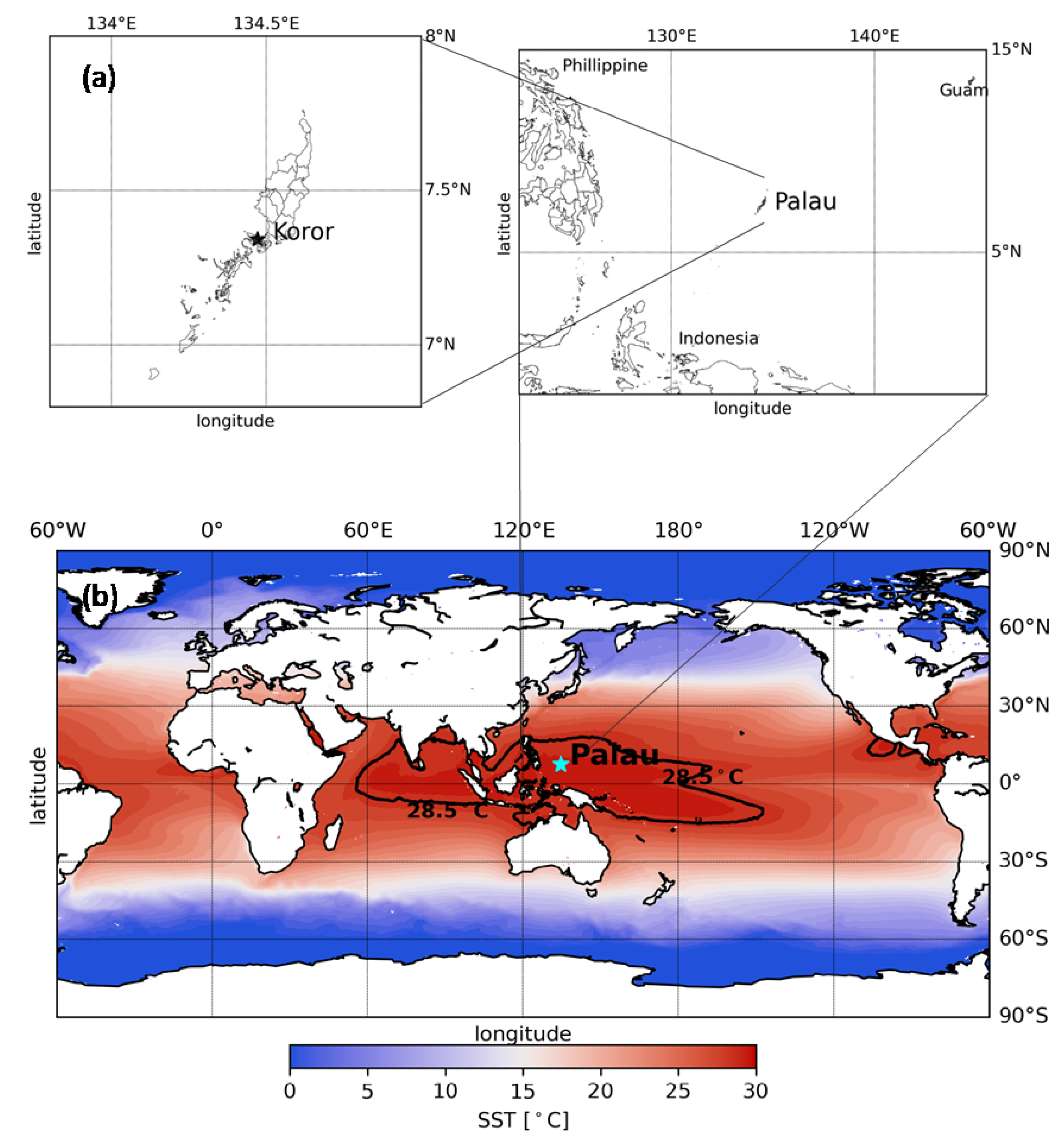
2.1. Site: The Palau Atmospheric Observatory (PAO)
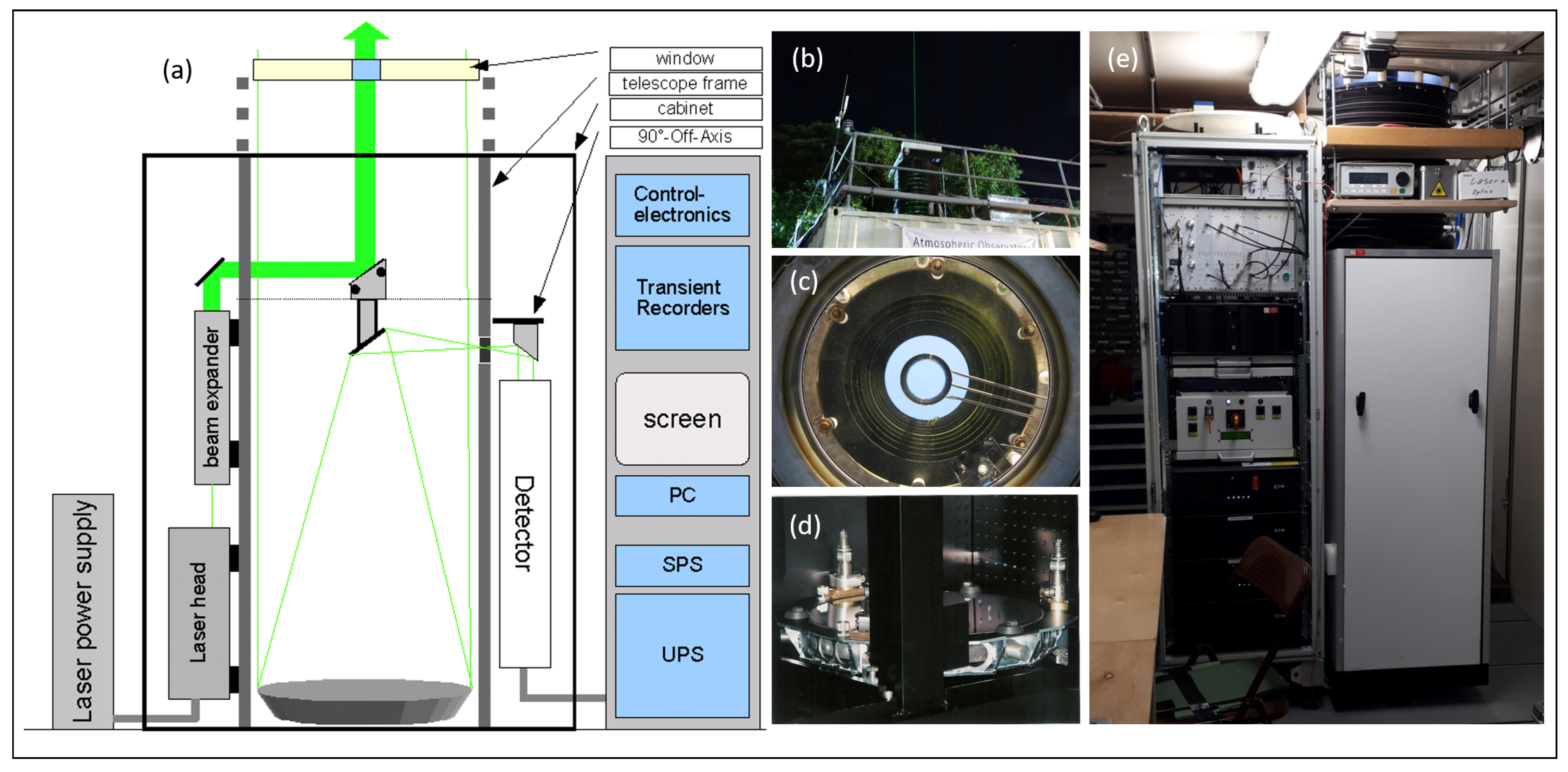
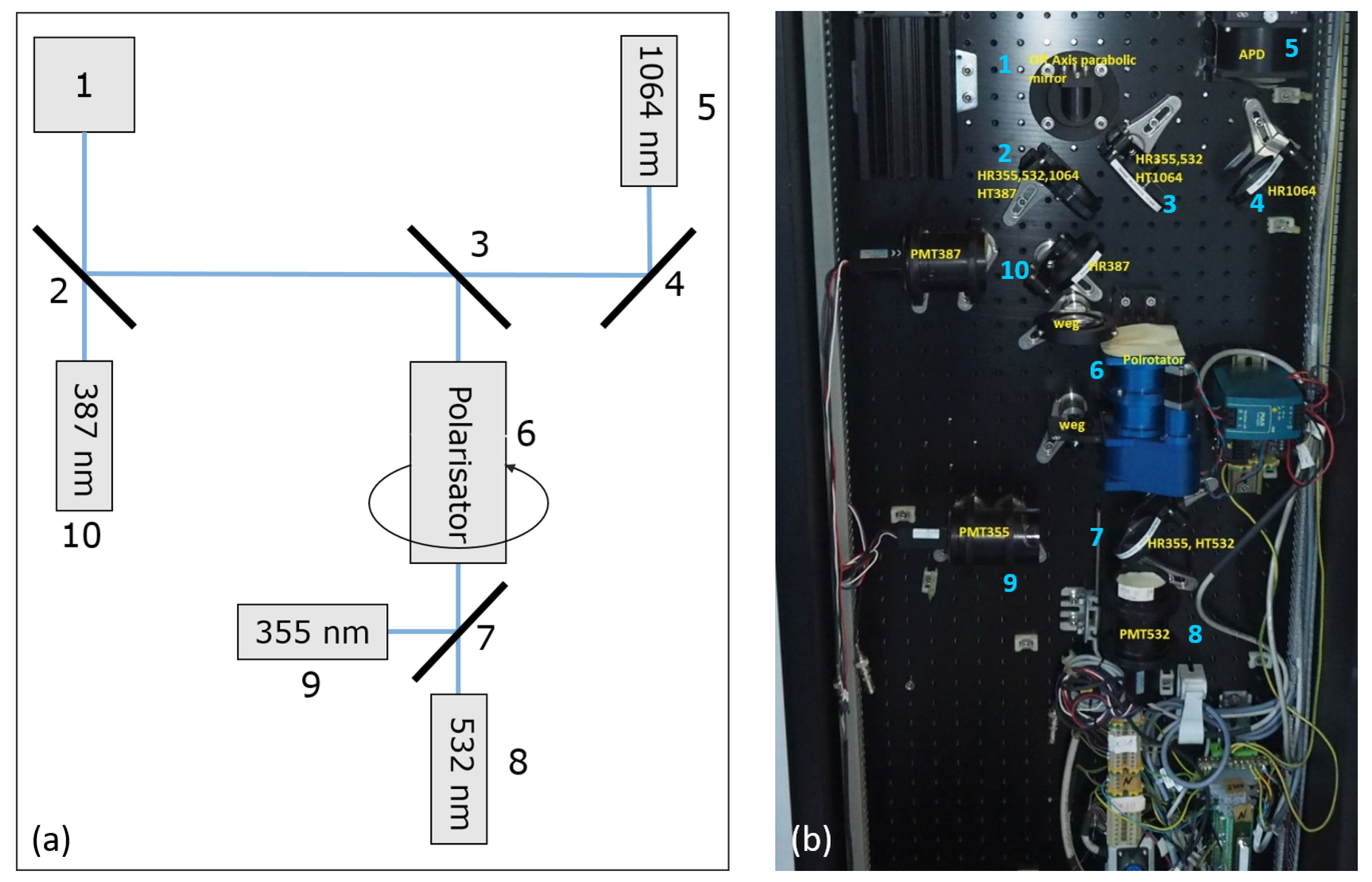
The Palau Atmospheric Observatory (PAO) [39,40] was established in 2015 at the Palau Community College (PCC), in downtown Koror (7.3°N, 134.5°E), Republic of Palau, see Figure 1a. The island country is located in the TWP region, which has the highest sea surface temperature (SST) higher than 28 °C all year, as shown in Figure 1b. Since 2018, lidar measurements by the Compact Cloud-Aerosol Lidar (ComCAL) have been conducted and funded by the Alfred Wegener Institute (AWI) at the PAO with contributions from the Institute of Environmental Physics (IUP), University of Bremen. This study focuses on the cirrus cloud detection in the TTL.

2.2. Instruments

2.2.1. Lidar System

The Lidar system, ComCAL, is part of the PAO [39] located in the center of the tropical Western Pacific warm pool. The lidar system has been operated since April 2018 and continued measuring until May 2019. Due to technique issues, no measurements exist between May 2019 and March 2022. After maintenance, ComCAL started operating from March 2022 until December 2022. In this study, we used lidar measurements obtained in two distinct periods: from April 2018 to May 2019, and additional data collected during March, July, and August 2022. It is worth noting that the setup of the lidar system remained consistent across both periods. Therefore, we integrated all available data, i.e., a total of 332 h of data over 124 days, to present the results. While there may be some variations between the two measurement periods, we assume that the overall characteristics of cirrus occurrence remain relatively consistent throughout the four years. Details of the month, year, and seasonal divisions are given in Table 1, and the monthly operation hours of the ComCAL lidar system are given in Appendix A. It is worth noting that due to (flight) regulations, we are not allowed to operate the laser between 10:00 and 15:00 local time, so measurements are taken outside of this period. We assume that there is no dominant diurnal feature of the cirrus cloud over Palau as Cairo et al. [38] suggested.
The Lidar system was developed by Immler et al. [42]. In the following, we briefly introduce its mechanical and optical design, including the newest modifications from the original setup. It was built for working in field campaigns on the ground or mobile platforms, for example, ships. It was also designed for automatic operation, allowing one to leave it without continuous maintenance, but only with regular attendance several times a year. The telescope of ComCAL is designed in Newtonian configuration with sending and receiving optics mounted on one rigid frame. As shown in Figure 2, the optical components are all held in one telescope frame to ensure the stability and limited set-up of the optical components (Figure 3).
The light pulses are vertically emitted by an Nd:YAG Laser (Quantel Brilliant, impres GmbH, Bremen, Germany) at three wavelengths—1064 nm, 532 nm and 355 nm—and the specification of the elastic detector channels are shown in Table 2. A parabolic mirror collects the backscattered light from the atmosphere. The received light is then redirected by the flat secondary mirror in a breadboard that contains the detector optics (see Figure 3). A 90° off-axis parabolic mirror deflects the light by 90° while parallelizing it. In total, four dichroitic mirrors separate the light in 355 nm, 532 nm, and 1064 nm (and the Raman shifted 387 nm, which is not used in our study). While the light at 1064 nm is directly detected by an Avalanche Photo Diode (APD), the light at the wavelengths of 532 nm and 355 nm passes through a rotating Glan–Taylor prism that is synchronized with the laser (Figure 3). In this way, the light polarized parallel and perpendicular to the laser polarization is alternately detected. Because the same detection channel is used for both polarization directions, this configuration enables a depolarization measurement without needing calibration. The signals are recorded by Licel transient recorders (20 MHz, 12 bit) in analog and photon counting (PC) mode simultaneously. The raw resolution of the ComCAL system is 135 s/7.5 m (time/altitude), and the used resolution is 10 min/60 m for BSR retrieval. The vertical range of the profiles is in principle from the ground up to 25 km.

2.2.2. Ozonesonde and Radiosonde

Electrochemical concentration cell (ECC) ozonesonde and radiosonde launches have been conducted at the PAO to measure the profile of O3 and meteorological profiles, such as the temperature, air pressure, and relative humidity of the atmospheric environment since 2016. For more detailed descriptions about the ozonesonde measurements, please refer to Müller et al. [39]. At least two ozone sondes are launched per month. Vaisala radiosondes were used for data transmission, measuring pressure, temperature, and humidity, and providing the GPS coordinates, the model RS92-SGP [43] until October 2017, the model RS41-SGP [44] after. The pressure and temperature profiles from the radio sondes are used to obtain the air number density via the law of ideal gas [45] (will be discussed in the following Section 2.3.1) combined with lidar measurements because of their high vertical resolution.
Other types of meteorological profiles are obtained from radiosondes launched by the US National Weather Service (under NOAA, National Oceanic and Atmospheric Administration) in Palau (station reference number: PTRO 91408, http://weather.uwyo.edu/upperair/sounding.html, accessed on 12 April 2024). The launch site was located close to the PAO until August 2018, before it was moved to the national airport, approximately 8 km away. Radiosondes are launched twice daily. The temperature and potential temperature profiles measured by the Palau weather station are used to derive the level of the TTL (see Appendix D) over Palau and the meteorology properties of cirrus clouds, such as temperature at the cloud layers.

2.3. Method

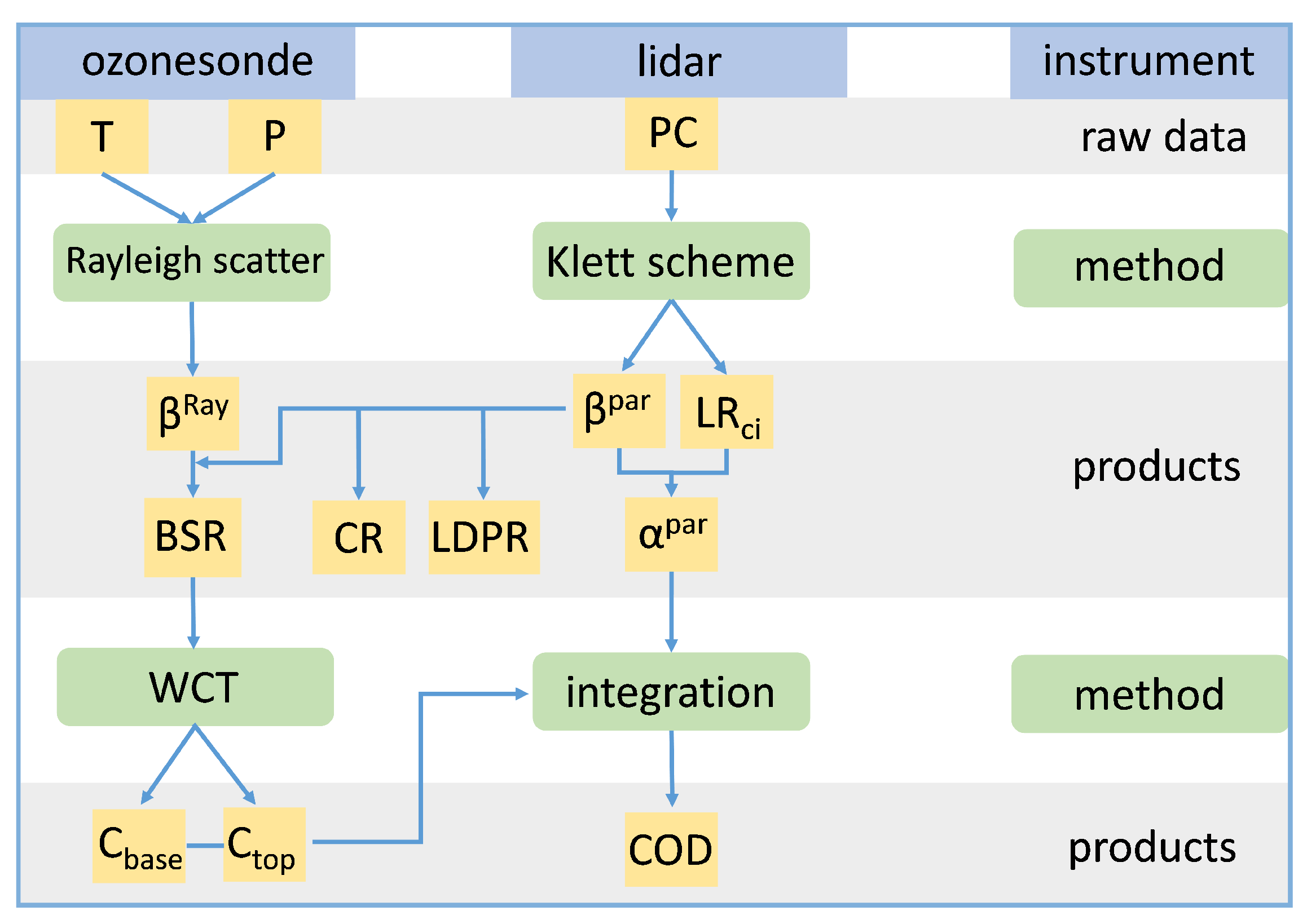
2.3.1. Retrieval of Properties of Cirrus Cloud

To retrieve the optical properties of the cirrus cloud, such as backscatter coefficient ( β ), extinction coefficient ( α ), and cloud optical depth (COD), we use the Klett optical characterization scheme [46] (refers to Klett scheme hereafter) to obtain the solution of the lidar equation. First, the lidar ratio ( L R c i ) of the cirrus cloud layer was needed. An average LR of 36/35 sr at 532/355 nm has been assumed for the background atmosphere, and then the LR is defined as the ratio of the extinction and backscatter coefficient of particles, e.g., aerosol and cloud, α p a r and β p a r , respectively:
L R ( λ ) = α p a r ( λ ) β p a r ( λ )
In order to obtain the lidar ratio of cirrus cloud ( L R c i ), a constrained Klett scheme was employed based on the backscatter ratio (BSR), which is defined as the ratio of the total and the molecular backscatter coefficient, which is β t o t a l ( λ ) and β R a y ( λ ) , respectively:
B S R ( λ ) = β t o t a l ( λ ) β R a y ( λ )
where β R a y ( λ ) is the scatter of the gases, widely known as Rayleigh scattering [45]. It is calculated by the air number density via the law of ideal gas [45] from radiosonde data (Section 2.2.2). When light is scattered by one atmospheric constituent, it can no longer interact with other components. Therefore, the total backscatter β t o t a l ( λ ) is simply the sum of contributions of the individual components:
β t o t a l = β p a r + β R a y
So the Equation (2) can be rewritten as:
B S R ( λ ) = 1 + β p a r ( λ ) β R a y ( λ )
The L R c i was first chosen independently by the assumption for cirrus clouds (typically around 17/29 sr at 355/532 nm) within the cloud layers. Based on the assumption that the atmosphere beneath the cirrus cloud layer was invariable, this value L R c i is iteratively inspected during the data processing to adjust the L R c i accordingly until the BSR matched with a reference BSR value beneath the cirrus cloud layer. To see more details about the constrained Klett scheme, please refer to Nakoudi et al. [47] (Figure 4), and based on this scheme, we applied it to the ComCAL measurements in Palau.
The scheme yielded the constant L R c i within the cirrus cloud layers vertically. Then, the COD can be calculated subsequently:
C O D ( λ ) = C b a s e C t o p α p a r ( λ ) = C b a s e C t o p L R c i · β p a r ( λ )
Then, the linear particle depolarization ratio ( L P D R , indicating the sphericity of ice crystals [48]) and color ratio ( C R , indicating the size of the ice crystals [48]) were calculated for each cirrus cloud layer, respectively:
L P D R = β p a r ( λ ) β p a r ( λ )
C R ( λ 1 , λ 2 ) = β p a r ( λ 1 ) β p a r ( λ 2 ) , λ 1 < λ 2
where L P D R is calculated from the ratio of the particle backscatter coefficient β p a r for light perpendicularly polarized ( β p a r ( λ ) ) to the backscatter coefficient parallel polarized ( β p a r ( λ ) ) to the laser. And, C R ( λ 1 , λ 2 ) is calculated from the ratio of particle backscatter coefficient β p a r at two different colors, i.e., λ 1 and λ 2 , and in this study, λ 1 = 355 nm, λ 2 = 532 nm. The size of the particles detected by multi-wavelength lidar can be roughly determined by calculating the CR from the two wavelengths used by the lidar system, similar to the Ångström [49] exponent, a rough estimate of the particle size. The simple relationship between the particle size and CR is that the larger the particle size, the closer the CR approaches 1 [48].

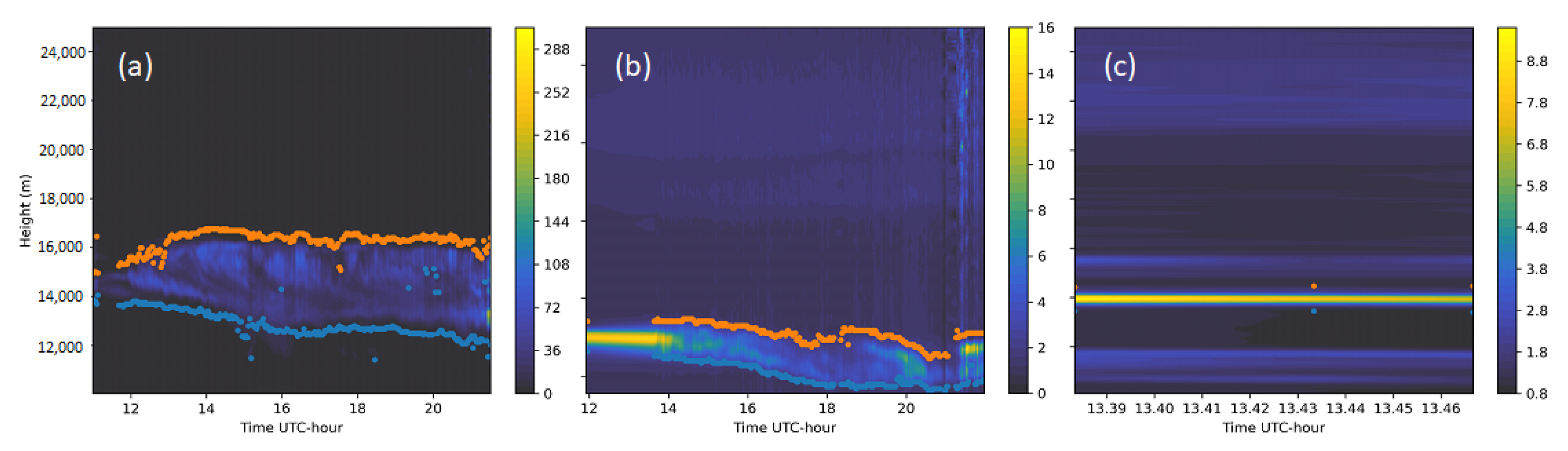
2.3.2. Detection of the Cirrus Cloud Layer from Lidar

As mentioned earlier, when particle scattering is negligible, i.e., under clear-sky conditions, the value of BSR is approximately equal to 1. Therefore, the base C b a s e and the top C t o p of the cirrus cloud can be determined from the BSR profiles as a function of altitude, measured by lidar from the inflection points of the BSR. The cloud detection method we use is the wavelet covariance transform (WCT) method, which is based on an integral quantity that is sensitive to the vertical gradient of the lidar signal. Since the signal-to-noise ratio (SNR) in the upper troposphere is typically low [47,50], the WCT method compares favorably to the method based on the differentiation technique in vertical layers based on the direct analysis of a specific threshold of BSR [50]. The WCT method has been used in determining the planetary boundary layer top height [51] and several similar studies for the detection of cirrus clouds, e.g., by Nakoudi et al. [52], Voudouri et al. [53], Pandit et al. [35]. The cloud detection method in this paper is specified as follows.
The coefficient W ( a , b ) is the result of the convolution between BSR and a zero-order wavelet function (Haar function), and is defined by the following equation:
h ( z b a ) = + 1 , b a 2 z b 1 , b z b + a 2 0 , e l s e w h e r e
where a and b are the width and the dilation of the wavelet, respectively. The coefficients W ( a , b ) , which are the convolution results between the B S R ( z ) and h ( z b a ) , are:
W ( a , b ) = 1 a z a / 2 z + a / 2 B S R ( z ) h ( z b a ) d z
If BSR is in phase or anti-phase with the Haar wavelet, the convolution result shows a local maxima or minima of the B S R ( z ) as a function of z. Thus, this can be used to determine the inflection point of the BSR, which corresponds to the bottom or top of the cirrus cloud. The parameter a is chosen as 500 m, and sensitivity studies show that the change in the value a between 300 m and 900 m does not show major effects on the determination of the cirrus cloud boundaries. The parameter b is the height step in the altitude range where the inflexion points of the BSR are. Thus, the range of the value b should be the altitude range where the signal of the cirrus cloud occurs. Above 10 km altitude, the cirrus clouds are known to be ice clouds, so we take 10 km as the minimum value of the parameter b, following a previous study by Cairo et al. [38]. The maximum value of b is 20 km, which is chosen as the upper detection limit of cirrus clouds.
Another important parameter is the threshold W t h . The altitude at which the values of W exceed this threshold represents the bottom or top of the cirrus cloud. A dynamic method based on the local maxima of W was applied to determine the threshold of WCT ( W t h ), which represents the C b a s e and C t o p . It is calculated by:
W t h ( t o p ) = max W max W 10
W t h ( b a s e ) = min W + min W 10
Figure 4 shows three examples for determining the C b a s e (blue dots) and top C t o p (orange dots) with BSR by the WCT method. All three cases with different geometric thickness cirrus cloud layers are detected accurately. For cases with more than one cloud layer, we first use this method to obtain the first layer, and then remove the first layer. After that, we use the same method again to the WCT profile without the signal from the first layer until no cloud layer can be filtered out. Please see details in the Appendix B.
Summarizing this and the previous Section 2.3.1, the steps of the scheme to retrieve the properties method of the cirrus for ComCAL are given in the diagram shown in Figure 5. There are several steps to control the quality of the products of ComCAL:
  • Before applying the scheme, a pre-screening based on the lidar profile in PC mode is performed to avoid profiles that may have problems like dead time, electronic noise, and background illumination effects [47]. In this study, only the lidar profile in PC mode with an acceptable signal-to-noise ratio (>3.0) in 10–20 km is further analyzed and included in the final dataset products of ComCAL.
  • The assumption of LR in the particle layer poses a challenge in real-world scenarios where LR varies vertically due to factors like aerosol particle size, refractive index, and shape. For example, LR can range from approximately 20 sr in the lower troposphere with marine aerosols to 100 sr when combustion aerosol particles are present at higher altitudes [54,55]. In our study, only cirrus cloud layers are considered. Thus, to avoid errors introduced by the assumption of L R c i , cirrus layers with unexpectedly high L R c i (>50) were screened out.
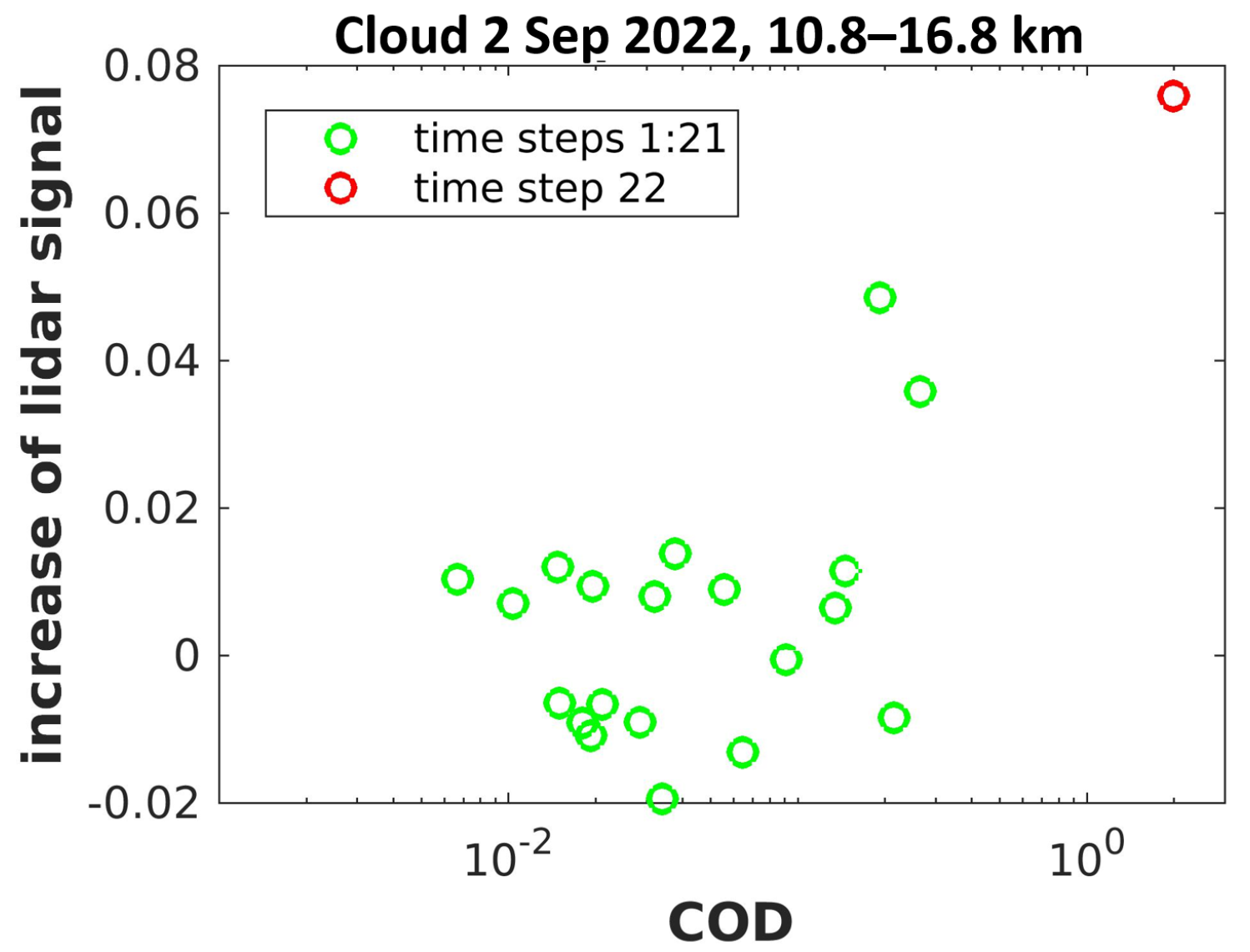
  • The effect of the multiple scattering (MS) is considered depending on the telescope field of view (FOV) of the lidar, the COD, and the altitude of the cloud. The higher the cloud, the thicker are laser beam and FOV, so it becomes easier for the photons to stay in the beam or FOV even after scattering. Different methods have been introduced to correct the MS (e.g., Hogan [56] and Eloranta [57]). Since no clear and straightforward method can be used to correct for MS to date, but only adaptions of single scattering to MS, we made tests to ensure that the uncertainty below 9% for COD value less than 2, as can be seen in details in Appendix C. Based on the sensitivity analysis, the cases of the cirrus cloud layer with COD higher than 2 were screened out to control the effect of MS on the quality of the retrieved properties.
After these steps, the maximum error for each variable retrieved from ComCAL measurements, e.g., the vertical profiles of the aerosol backscatter coefficient β p a r ( λ , z ) at 532 and 355 nm in parallel and perpendicular polarization as well as at 1064 nm, is given in the data product along with the measurement results of β p a r ( λ , z ) . The products of ComCAL in August 2022 during the Asian Summer Monsoon Chemical & Climate Impact Project (ACCLIP) campaign are now publicly available in the UCAR/NCAR-Earth Observing Laboratory (EOL) [58]. Please refer to Data Availablity for data access for other periods.

3. Results

3.1. Cirrus Occurrence over Palau

We detected cirrus cloud layers and integrated all available data, i.e., a total of 332 h of data over 10 distinct months, to present the results of the occurrence of cirrus over Palau. Understanding the seasonal cycle of the cirrus cloud layers is crucial to assessing the impact of cirrus clouds on regional climate. In order to achieve this, the monthly percentage occurrence (PO) of cirrus clouds at different altitude levels is calculated using ComCAL lidar cloud layer measurements. This calculation involves determining the ratio of profiles with cirrus clouds t m o n ( z ) at a specific altitude bin z to the total number of profiles available t m o n and it is calculated by:
P O m o n ( z ) = t m o n ( z ) t m o n z = 10.0 , 10.1 , 10.2 , 20.0 km
where P O m o n ( z ) is the monthly percentage occurrence of cirrus clouds at each altitude bin z of 0.1 km from 10 km to 20 km, which is calculated by the ratio of the t m o n ( z ) and t m o n . The value of PO is used to study the occurrence of cirrus clouds during the specific measurement period as a function of altitude. t m o n ( z ) represents the sum of the total measurement times of the data collected individually within each month of the year for each altitude bin in which cirrus clouds were detected. t m o n represents the total observation time of the lidar system in each month.
Seasonal PO for cirrus clouds can be calculated if the time in the Equation (12) is replaced with the sum in seasons. It should be noted that no observations were made in June and November due to technical lidar issues. In this paper, we use July and August data to partially represent summer and October and November to represent autumn. The specific months and years with the seasonal division of the dataset are given in Table 1.
The time series of the monthly PO of cirrus clouds in Palau from April 2018 to August 2022 is shown in Figure 6. The number of cirrus layers detected each month by Lidar is shown by the number below the monthly columns in Figure 6. For details about the total measurement time of the lidar and cirrus cloud occurrence in each month, please see Appendix A. The peak altitude of PO occurs in the range of 15 km–18 km in most months, except for May. This indicates that cirrus clouds frequently occur in the upper part of the TTL (above 15 km). The C t o p is close to the cold point tropopause (CPT), while C b a s e is consistent with the lower boundary of the TTL, the level of neutral buoyancy (LNB). The level of the minimum stability (LMS) is also presented in Figure 6, to see the lowermost part of the TTL. The cloud occurs less frequently in LMS. But for May, it is seen that the LMS and the altitude of the maximum PO are lower compared with other months. This anomaly is consistent with high monthly anomalies from the annual mean of the ozone volume mixing ratios at this altitude in May [39], and needs to be studied further. The seasonal pattern of the height of the cirrus cloud layer and the peak of PO is consistent with the CPT, with minimums in July and August then increasing in height until December, and stable from January to March next year, then reaching maximal height in April. More details about the TTL features are given in the Appendix D.
On a monthly basis, as shown in Figure 7, the annual and seasonal PO is quantified in each season by Equation (12) for each month replaced with total measurements and each season. The maximum annual PO of cirrus clouds is 22% at about 16 km and 1 km beneath the height of the CPT. For winter, the seasonal PO is the largest with a peak in 16 km of 42%. For the frequency of cirrus above the CPT, the seasonal PO in winter has the largest frequency (maximum of 30%) above CPT compared to other seasons, followed by spring, autumn, and the least in summer (less than 10%). In spring, there are two peaks of PO in the TTL, one at around 13 km and another slightly above or around the CPT. This feature in spring is different from other seasons with only one peak below the CPT height. The previous one-month campaign conducted by Cairo et al. [38] in Palau during the spring season also reported this two-peak feature of the cirrus cloud which may indicate the Madden–Julian oscillation (MJO) in this spring season over the TWP region.

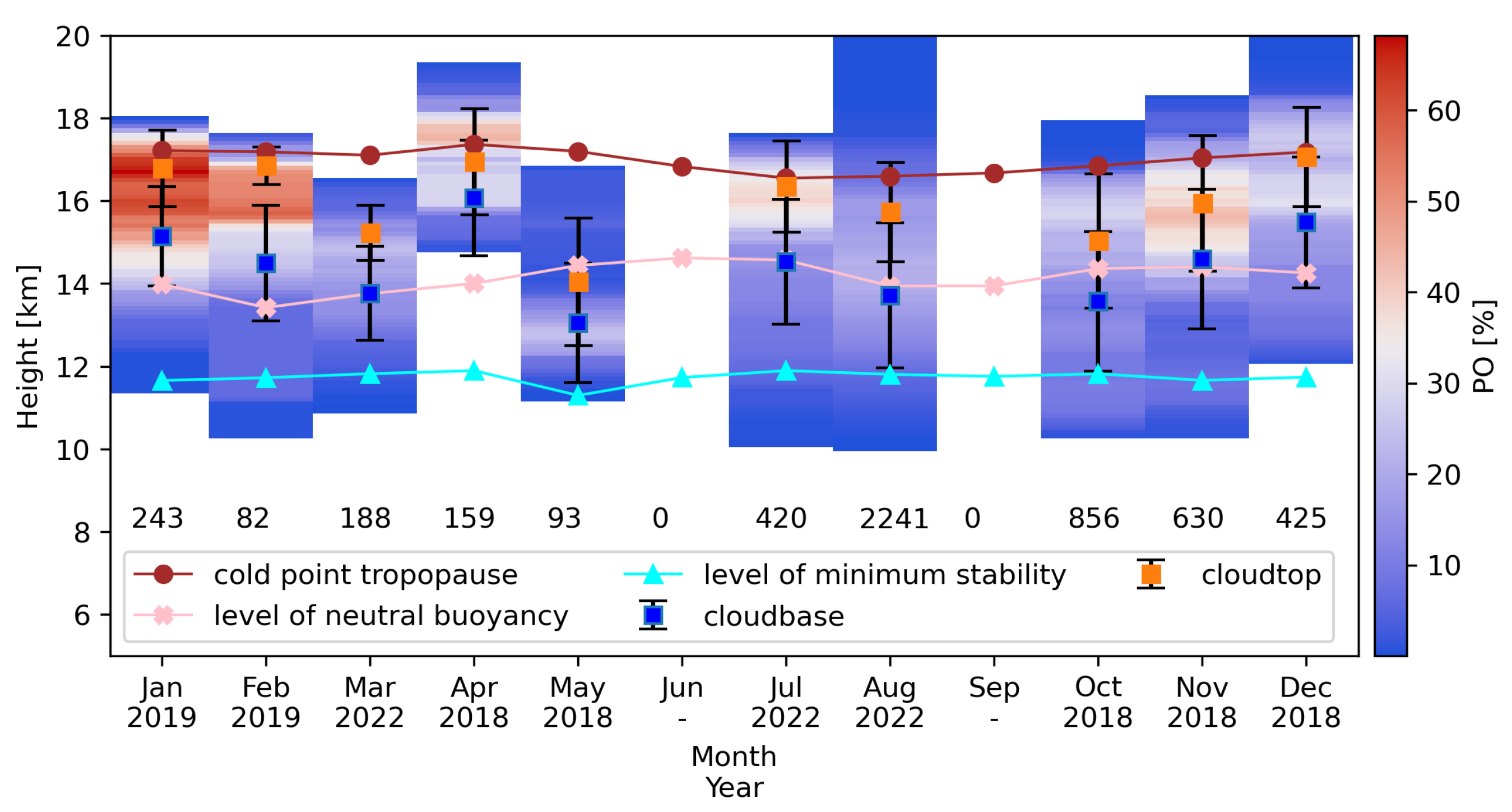
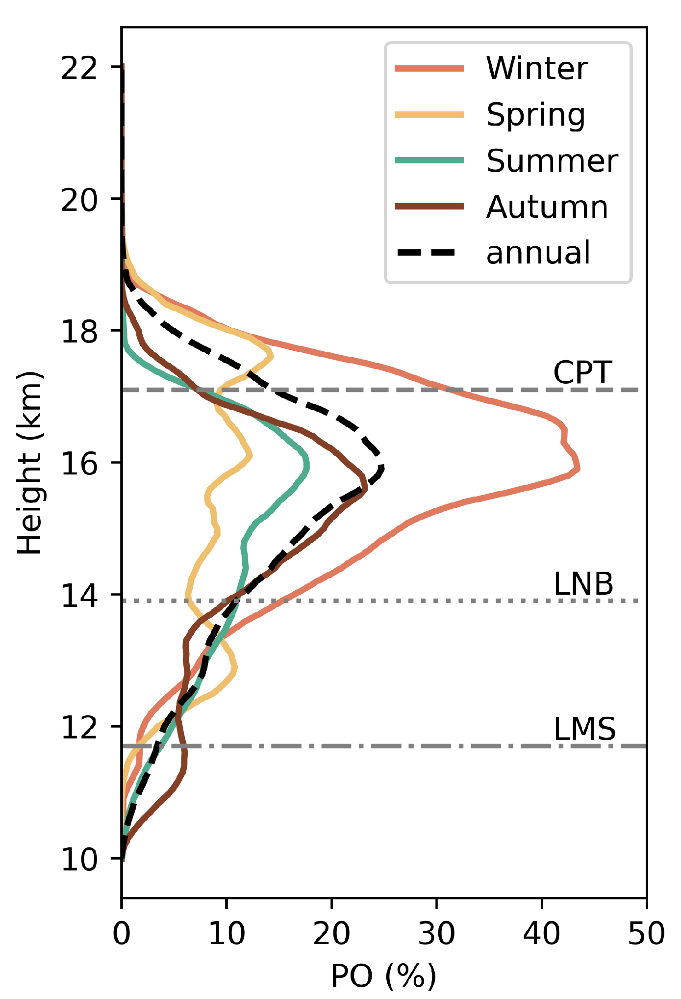
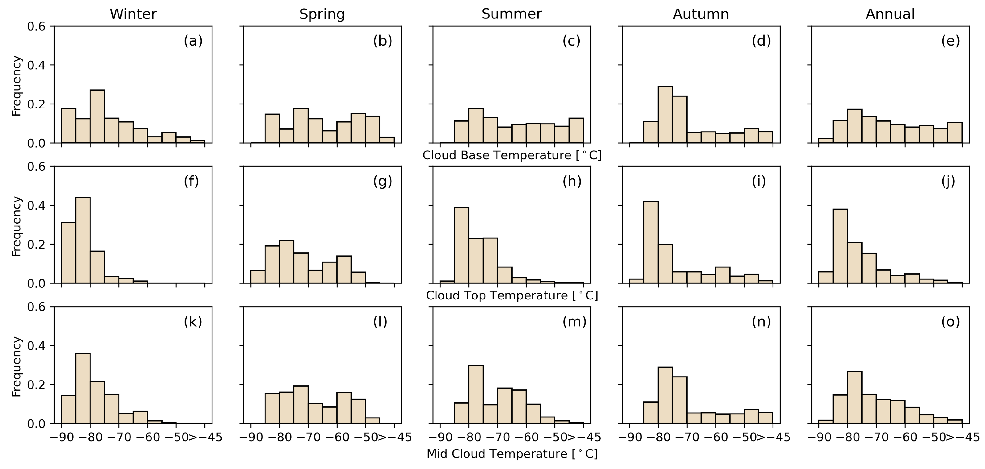
3.2. Geometrical and Thermodynamic Properties

The frequency of the occurrence of geometrical properties, which are the geometrical thickness (GT), cloud base, and cloud top height, is shown in Figure 8. Additionally, the thermodynamic properties, which include the cloud base top temperature and mid-cloud temperature, are illustrated in Figure 9. The seasonal divisions of the dataset are given in Table 1. The statistical details are given in Table 3.
The geometrically thinnest cirrus layer is in spring (mostly less than 2 km), followed by autumn and winter, and the geometrically thickest in summer, as shown in Figure 8a–e. Only in winter and summer, the GT is more than 4 km with a frequency of 2% and 10%, respectively. The annual averaged GT of cirrus is mostly distributed between 1 and 2 km with an annual average of 1.4 ± 0.7 km (see Table 3), and only a few cases more than 4 km.
The distribution of the cloud base height is spread between 10 and 18 km, as shown in Figure 8j. In winter, the height of the cloud base is slightly higher than in the other seasons with an average value of 15.3 ± 1.4 km (see Table 3), compared with around 14 km in other seasons (Figure 8f–j). For the distribution of cloud top (Figure 8k–o), the annual peak is 17 km. The higher the cloud top, the more frequent they become, except in spring, where we see a second maximum below 13 km. In winter, the probable range of the height of cloud tops is narrower between 14 and 17 km, compared with other seasons between 12 and 17 km.
The temperature of the cloud is derived from the radiosondes launched each day at 12 h UTC by the National Weather Service of Palau (see Section 2.2.2). The cloud layers are matched with the temperature profiles launched at 12:00 UTC/21:00 local time. As shown in Figure 9a–e, the cloud base temperature is evenly distributed between 85  °C and 45  °C with a frequency of around 0.1–0.2, and the average cloud base temperature is 71.7 ± 11.5 °C (see Table 3). For the cloud top temperature, the most probable temperature is within the range −85 °C and −80 °C with a frequency of about 0.4, as shown in Figure 9f–j. This is an exceptionally low temperature and approaches the temperature of the annually averaged CPT (−83.8 °C, see Appendix D). Except for spring, the highest frequency ranges of cloud top heights in the other three seasons were all between 85  °C and −80 °C, and the frequencies all reached 0.4. As for the mid-cloud temperature, shown in Figure 9k–o, the distribution is similar to the cloud top temperature. The coldest cirrus layer is in winter when the tropopause is coldest. The mid-cloud temperature of less than 85  °C only occurred in winter with a frequency of 0.14. The annual mean of the mid-cloud temperature is −73.8 ± 9.8 °C.

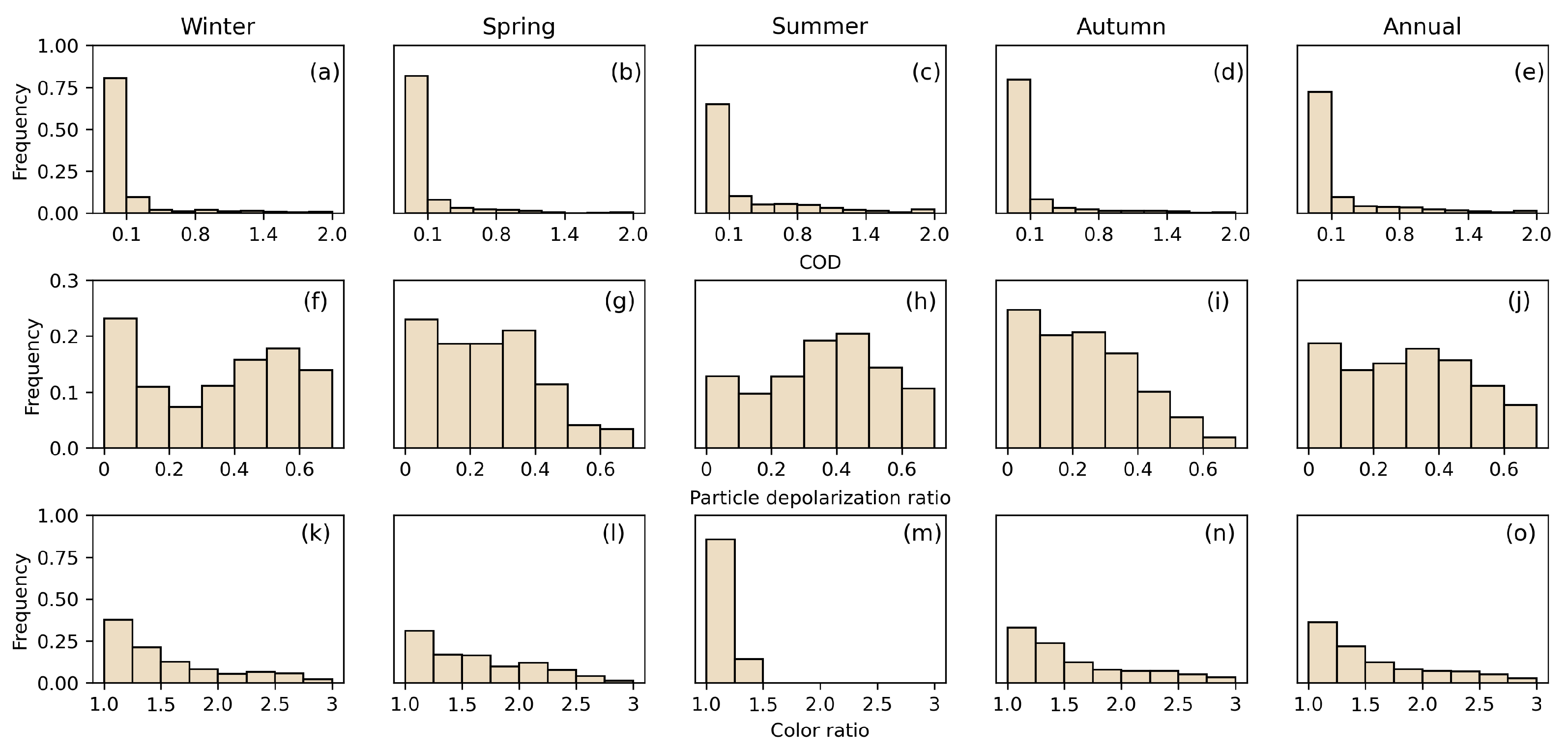
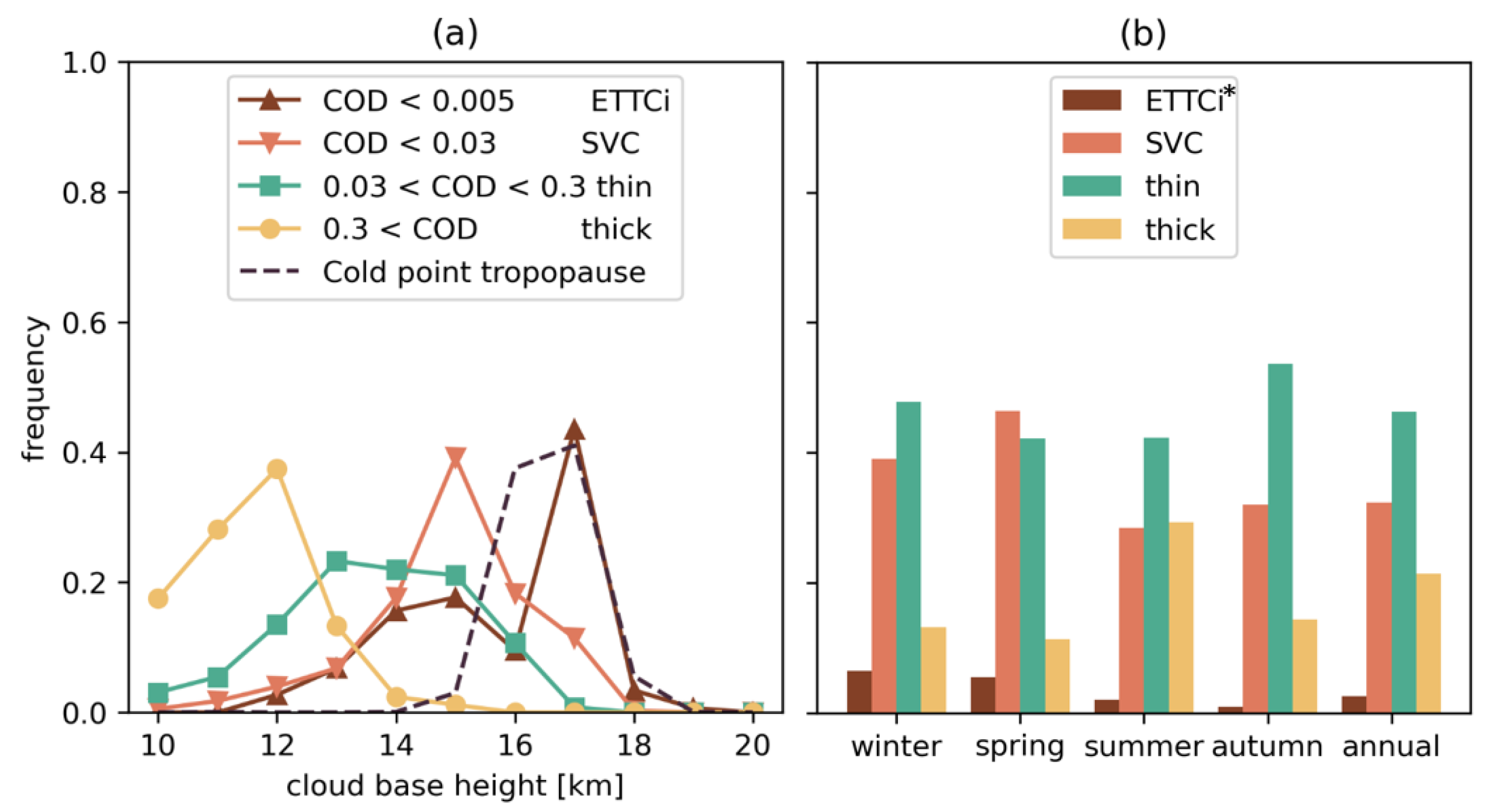
3.3. Optical Properties

An overview of the optical properties of cirrus including cloud optical depth (COD), depolarization, and color ratio (CR) are presented in Figure 10 and the statistical details are listed in Table 3. According to our measurements, the COD is distributed in a broad range with a minimum of 0.001 and a maximum of 2.1. It can be seen from Figure 10a–e that the COD is mainly within the range of 0–0.2. In all seasons, the fraction of a COD between 0 and 0.1 is about 0.75. The annual average COD is 0.25, and only in summer, the average COD is larger than 0.3, followed by 0.19 in autumn and the winter, with the lowest COD in spring, see Table 3. From the frequency distribution, compared with other seasons, only summer has a larger number of clouds with a COD of 0.3–0.5 (Figure 10c).
The depolarization ratio is ranging from values very close to zero to 0.69. As shown in Figure 10f–j, the frequency of the range 0–0.1 is slightly larger than other ranges, about 0.19, followed by the range 0.3–0.4, about 0.18. The depolarization ratio is slightly lower in spring and autumn than in winter and summer. However, all seasonal averaged values of the depolarization ratio are close to 0.3 (Table 3), which indicates that the ice cloud particles are irregular in most cases.
As for the CR, as shown in Figure 10k–o, it varied mainly between 1.1 and 2.5, with an annual average of 1.6 ± 0.5. In summer, the CR is much lower than in other seasons, with a high frequency (0.85) of CR between 1.1 and 1.25. This indicates that there are larger ice particles during summer than in other seasons. During the monsoon season, when Palau is located in the south of the CE or the transition area [19], the TTL is humid and warm because of the intensive convective activities during this time. Under this circumstance, a great amount of deep convective cells occur in tropical oceanic regions and generate the spreading anvils and long-lived cirrus with larger particle sizes compared with the other seasons.

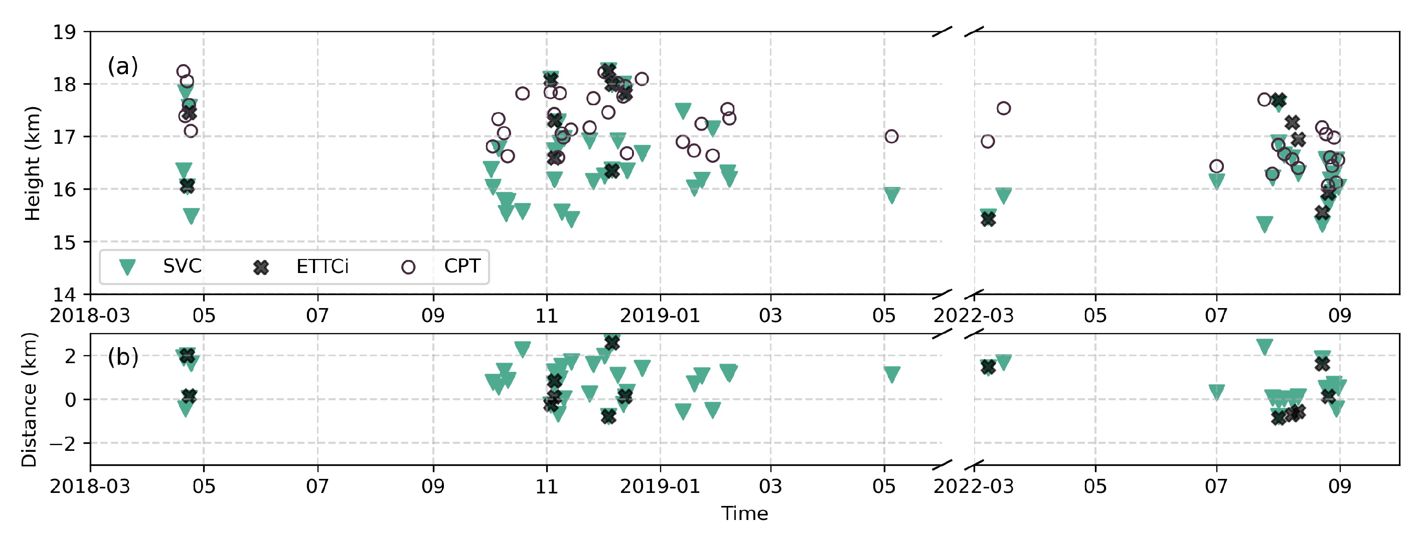
3.4. Cloud Layer and the Tropopause

Figure 11a shows the frequency of clouds with different values of COD against the cloud base. Visible thick and thin cirrus occurred between 12 and 14 km, and the cirrus became optically thinner at higher altitudes. SVC usually occurred in 16 km which is lower than the CPT at around 17 km. As mentioned in Section 1, we use a subdivision definition of the cirrus cloud of COD less than 0.005, which is an Extremely Thin Tropical Cirrus (ETTCi), adapted from Immler et al. [9]. ETTCi accounts for 1.6% of the total number of cirrus measured over Palau, and the most frequent altitude of 18 km for ETTCi is even higher than the peak of CPT (17 km, see the dashed line in Figure 11a). The dehydration of tropospheric air before it enters the stratosphere is associated with the occurrence of ETTCi [9].
The seasonal and annual occurrence of the different types of cirrus is shown in Figure 11b. The most prevalent type of cirrus in Palau is the optically thin cloud accounting for 47%, followed by SVC (32%) and thick cirrus (22%), and the least is ETTCi (1.6%). The SVC has a higher frequency of occurrence in spring and winter than in summer and autumn. In summer, thick cirrus and SVC appear at almost the same frequency (about 28%), which is also the season with the highest frequency of thick cirrus.
As mentioned in Figure 11a, the optically thinner clouds tend to stay at a higher altitude. The most frequent mid-cloud height of the ETTCi is 18 km, which is even higher than the CPT. In order to analyze the relationship between mid-cloud and CPT height in different seasons in detail, the distance from the mid-cloud height of clouds grouped by COD to the CPT height is calculated and shown in Figure 12. The CPT height is calculated from the daily temperature profiles measured by radio soundings launched over Palau (as mentioned in Section 2.2.2). Then, the CPT height and the cloud layers are matched with the time when the lidar is operating. The distance from CPT to the height of the mid-cloud layer is calculated by:
d C i r r u s = H C P T H M i d c l o u d , H M i d c l o u d = ( C i r r u s b a s e + C i r r u s t o p ) / 2
where d C i r r u s is the distance from CPT to the mid-cloud height of cirrus cloud layers measured by Lidar. The height of the mid-cloud height ( H M i d c l o u d ) is the average height of the cirrus cloud base and top derived from the same measurement time point. For simplicity, for example, the distance from CPT to the mid-cloud height of SVC and ETTCi cirrus cloud is referred to as d S V C and d E T T C i , respectively.
During the lidar sampling time, the SVC and ETTCi are both close to the CPT, with d S V C and d E T T C i around 2 km, indicating that these cloud layers stay beneath or above 2 km near the CPT. However, ETTCis are closer to the CPT and have more days higher than the CPT with d E T T C i < 0 , compared with SVC. The ETTCis are the rare cases measured over Palau compared with other optically thicker cirrus and are usually observed during winter and summer for the given lidar sampling time. However, they are very important because they indicate STE. In winter, d E T T C i above the CPT indicates that the airmass transits into the stratosphere through the cold trap above the TWP region. Due to the exceptionally cold temperature in the upper TTL over Palau (as low as 185 K, see Figure A4) during this period, the dehydration process in the air mass favors its slow and continuous rise along with the formation of ETTCi. In summer, d E T T C i above CPT can be linked to the movement of the western Pacific monsoon and the chemical equator above Palau. This atmospheric circulation system can cause intensive convective clouds. The convective clusters excite the equatorial Kelvin waves which are highly related to the formation of the ETTCi [12].

3.5. Comparison of the Cirrus Cloud Properties in Different Tropical Sites

The cirrus clouds observed in Palau are colder compared with other places in the tropics. Table 4 shows an overview of the cloud properties at different tropical sites measured by lidar and from satellite measurements (Tropics ± 30°). The cirrus cloud layers detected in Palau have higher C b a s e and C t o p than all sites except for Nauru Island [17], which is also located in the warm pool, the western Pacific Ocean; its C t o p is 16.5–17.0 km similar to Palau. The temperature of the cirrus cloud layer in Palau is the lowest, which can be explained by the overall lowest temperatures in the TTL in the TWP region [20].
For optical properties, comparing the CR (annual mean of 1.6 ± 0.5) of cirrus clouds in Palau with similar studies, Voudouri et al. [53] reported CR (355/532) of 1.50 ± 0.80 in Gwal Pahari (28.43°N, 77.15°E) in India and 1.40 ± 1.10 in Elandsfontein (26.25°, 29.43°E) in South Africa, which is consistent with our results. This indicates that the particle sizes of the cirrus clouds between different tropical sites are similar. Cirrus above Gandanki (13.5°N, 79.2°E) shows a similar GT seasonal pattern to Palau, being geometrically thinner in spring and thicker in summer. The occurrence of thicker cirrus here is tied to the Asian summer monsoon, which is a notably distinct pathway, i.e., the Asian summer monsoon anticyclones for air masses to enter the stratosphere [35].

4. Discussion

A previous study based on the ground-based Lidar in Palau during the spring season by Cairo et al. [38] showed cirrus clouds occurring throughout the whole TTL with two defined peaks, one at 10–13 km and the other at or below the CPT. Our results for the spring season (MAM), see Figure 7, are partly consistent with this, showing one maximum in the occurrence at around 13 km and another slightly above or around the CPT. This is different from other seasons. As Cairo et al. [38] suggested, this spring feature is related to atmospheric temperature anomalies and the MJO. The optically thicker cirrus clouds were in a phase with the beginning and end of the MJO cycle in their study. The observations of clouds in the lower part of TTL (10–15 km) can be attributed to the enhanced convective activities affected by the planetary-scale Kelvin and Rossby waves in the stably stratified TTL induced by the MJO-related deep convection [38,62].
Previous studies based on satellite/ground-based Lidar focused on the tropic regions (e.g., [38,61,63]) have elucidated that seasonal variations in cirrus clouds in the TTL, specifically in the lower part (10–15 km), are profoundly influenced by the changing monsoon seasons and relatively dry periods. This variation in convective activities in tropical regions is typically reflected by the ITCZ [59,62] or the CE [19] which is another indicator of the interhemispheric exchange. Sun et al. [19] showed that the CE provides a more distinctive picture of the location of this exchange in the TWP. Our results of the optical properties, specifically CR, of the clouds also manifest a correlation between the convection zone and the cloud measurements. In summer (July–August), the CE is located in the latitude of Koror indicating an enhancement of the convective clouds induced by the converging zone. The west Pacific monsoon reaches Palau during this period and modulates transport patterns and the abundance of atmospheric constituents like ozone and water vapor [39,64]. The CR is significantly lower with an averaged value of 1.1 ± 0.1 (532/355 nm), see Figure 10k–o and Table 3) than in other seasons and the annual mean (1.6 ± 0.5, 532/355 nm) which indicates larger ice crystals. In addition, cirrus clouds observed during summer have a higher COD (see Figure 10). The observed cloud optical properties are consistent with enhanced convective activity, which is confirmed by the location of the CE and the influence of the West Pacific monsoon. This is also consistent with the Lidar measurements obtained in Gandanki (13.5°N, 79.2°E), India, which is influenced by the Asian summer monsoon [35]. In contrast, when the CE shifts south of Palau during other seasons, Palau is less influenced by large-scale convergence zones. Our measurements reveal a larger CR for cirrus clouds during this time, indicating smaller ice crystals and thus less deep convection. These high cirrus clouds are more likely to originate from in situ dry freezing [1,9,65].
Satellite-based studies showing increased cirrus cloud occurrence in the TTL during NH winter [1,66]. Zou et al. [66] reported the tropical cirrus clouds (±20°) above the tropopause in December–February with a frequency of 15% compared to 8% during summer (July–August). Relative humidity with respect to ice (RHi) from the flight measurements over the TWP region showed the highest RHi over the TWP, and the associated persistent cirrus formation during winter [24]. Schoeberl et al. [24] suggested that such a high RHi in the TTL during winter is associated with the adiabatic upward motion in the TWP region at about 17 km and induced ice cloud formation. Our measurements of cirrus clouds during winter are consistent with these previous results, with the coldest and highest cirrus cloud layer of the year. Moreover, the seasonality of the altitude distribution of different cirrus cloud types (Figure 7, winter) suggests that cirrus clouds in winter are also most frequently close to the CPT (about 30% of the total observations of that season). Additionally, compared with other sites in the tropical region (Table 4), Palau has higher C b a s e and C t o p and the lowest cloud temperature. Such features of the thin and cold cirrus above Palau indicate that the occurrence of this cloud is related to the dehydration process in the cold trap. By this process in the cold trap, the tropospheric air masses can enter the stratosphere through the large-scale uplift.
As previous studies suggested, the SVC is related to the dehydration of tropospheric air before it enters the stratosphere, serving as an implication for the location where air enters the stratosphere [67]. Our observations indicate that SVC also occurs around the CPT height over Palau but with several cases lower than the CPT height of about 17 to 18 km (Figure 11a and Figure 12). The occurrence of the ETTCi accounts for 1.6% of the overall cirrus cases over Palau with only 14 cases captured in our measurements. Most measurements (about 71%) ETTCi are above CPT and the highest frequency of the C b a s e of ETTCi is about 17 km, which coincides with that of the CPT height. This suggests that both these cirrus clouds and SVCs are very important and could potentially be indicators of the last dehydration process of the TTL air masses. Then, they rise further into the stratosphere through this process. Therefore, more measurements of ETTCi and SVC are needed to improve our understanding of the STE.
Compared with other stations in the tropics, the cirrus cloud layers detected in Palau have a higher C b a s e and C t o p , except for the island of Nauru [17], which is also located in the TWP region. The temperature of the cirrus cloud layer in Palau is the lowest corresponding to the lowest temperature in the TTL above the TWP region [8]. The results of the coldest cloud above Palau reveal a possible transport pathway from the TTL to the stratosphere [7,68]. As the pathways and mechanisms of tropospheric air masses across TTL and entering the stratosphere remain an active research question [24] our observations may be able to give further observational support to this research question.

5. Conclusions

We conducted an extensive analysis of cirrus clouds in the altitude range from 10 to 20 km using lidar measurements in Koror, Palau ( 7.3 ° N , 134.5°E) over the TWP region from April 2018 to August 2022. This study, despite a year-and-a-half gap (from mid-2019 to 2021), provides a comprehensive overview of cirrus properties in the TWP warm pool. Our lidar measurements totaling approximately 332 h after quality control partly fill the gap of the cirrus cloud measurements from the ground-based lidar in the TWP region.
The geometrical and optical properties of cirrus clouds were quantified across seasons. Cirrus occurrence over Palau is 47.9% of the total lidar sampling time, primarily in the upper TTL from 15 to 18 km and less frequent in the lower TTL from 12 to 15 km in most months. Geometrical thickness (GT) varies seasonally, being geometrically thinner in spring and thicker in summer. The most probable GT is 1–2 km, rarely exceeding 3 km. The cloud base ( C b a s e ) is evenly distributed from 10 to 18 km, while the cloud top ( C t o p ) is higher and closer to the CPT in winter. The seasonal cycles of cirrus heights—especially C t o p —and the CPT heights are consistent with the lowest altitude in July and August, before there is a gradual increase until December, stability from January to March, and a maximum in April (Figure 6). The annual mean of the mid-cloud temperature is −73.8 ± 9.8 °C. The most probable temperatures in the cirrus cloud layer are within the range of −85 °C and −80 °C, which agrees with the temperature of CPT. The mid-cloud temperature below −85 °C near the TTL minimum temperature only occurs in winter over the TWP region.
Cloud optical depth (COD) is mainly within the range of 0–0.2, with 70% having COD < 0.1 in all seasons. Most of the cirrus clouds observed by lidar over Palau were optically thin (46%), followed by sub-visible clouds (SVC) (32%), with optically thick clouds (22%) occurring least frequently. Slightly higher COD occurs in summer. The annual mean linear particle depolarization ratio (LDPR) of cirrus is 31 ± 19%, showing limited season dependence. The annual mean color ratio (CR) in 355/532 nm is 1.6 ± 0.5, and significantly lower in summer (1.1 ± 0.1) compared with other seasons with a CR of about 1.5, indicating larger ice particles formed during the summer monsoon season over Palau.
During lidar sampling, ETTCi often exceeds CPT, particularly in winter and summer, signaling its importance in indicating STE. In winter, the d E T T C i above CPT suggests an airmass transit into the stratosphere via the cold trap above the TWP region over Palau, while in summer, it reflects the influence of the western Pacific monsoon movement and the chemical equator above Palau, leading to convective cloud formation with overshooting tops.
Compared to other tropical sites (± 30 ° ) , cirrus over Palau has the highest C b a s e and C t o p and the lowest cloud temperature, consistent with the coldest TTL temperature over the TWP region in winter. This indicates that the occurrence of this cloud is related to this specific location where the pathway between the troposphere air into the stratosphere occurs. Further studies are needed to investigate these clouds and their connection to the pathway of air entering the stratosphere.
This work was motivated to provide observational support for the study of atmospheric transport in the upper troposphere and lower stratosphere (UTLS) region and validate the dominant pathways of the STE over the TWP region. From our measurements of cirrus in the upper air, the prevalence of the coldest cirrus layer correlates with the coldest temperature in the TTL. The continuous measurements to obtain optical and geometric properties, ETTCi and SVC, over the TWP are required to better understand the STE process. Further investigations using trajectory analysis and satellite observations are needed to link our measurements to the pathway of air entering the stratosphere over the TWP region.

Author Contributions

Conceptualization, C.R. and X.S.; methodology, C.R. and X.S.; software, C.R., X.S. and W.R.; investigation, X.S.; resources, W.R., I.B. and S.P.; data curation, X.S., C.R., D.J., K.M., I.B. and W.R.; writing—original draft preparation, X.S.; writing—review and editing, C.R., K.M., M.P., D.J. and J.N.; visualization, X.S. and C.R.; supervision, C.R., J.N. and M.P.; project administration, M.P. and K.M.; funding acquisition, J.N., M.P. and K.M. All authors have read and agreed to the published version of the manuscript.

Funding

This work has been supported by the BMBF (German Ministry of Research and Education) in the project ROMIC-II subproject TroStra (01LG1904A) and the DFG (Deutsche Forschungsgemeinschaft, German Research Foundation) project 404/27-1.

Data Availability Statement

The dataset related to this publication has been partly available (during the ACCLIP campaign, August 2022) in the UCAR/NCAR-Earth Observing Laboratory: https://doi.org/10.26023/SD3W-WKBH-5X13 [58]. Other data products of ComCAL are available upon request from the corresponding author. The ozonesonde dataset is available under https://doi.org/10.5281/zenodo.6920648 and will be included in the SHADOZ database in the future. The Palau weather station data (station code: PTRO 91408) was accessed via the upper-air sounding database provided by the University of Wyoming https://weather.uwyo.edu/upperair/sounding.html, accessed on 12 April 2024. The SST data in Figure 1 were accessed via the Goddard Earth Sciences Data and Information Services Center (GES DISC), https://disc.gsfc.nasa.gov/datasets/M2TUNXOCN_5.12.4/summary?keywords=tavgU_2d_ocn_Nx, accessed on 12 April 2024. All the data products and codes are available upon request from the corresponding author.

Acknowledgments

The authors want to thank Patrick Tellei, President of the Palau Community College, for the provision of space for the laboratory containers in the college; German Honorary Consul Thomas Schubert, for overall support; and Jürgen “Egon” Graeser (AWI) for operations at the PAO.

Conflicts of Interest

Authors Wilfried Ruhe and Ingo Beninga was employed by the company Impres GmbH. The remaining authors declare that the research was conducted in the absence of any commercial or financial relationships that could be construed as a potential conflict of interest.

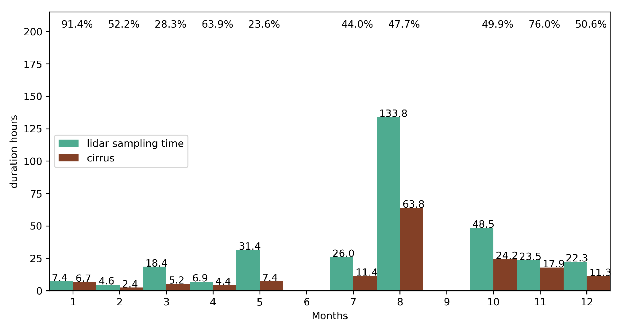
Appendix A. Measurement Hours of the Lidar System

The hours of the measurement time of ComCAL and the time of the cirrus cloud occurrence in each month are shown in Figure A1. The total measurement hours of the lidar system were 332 h during the period 2018–2022. Cirrus cloud layers are being detected in each month. The time of the occurrence of the cirrus cloud is also shown each month with the total measurement time of the lidar system. There were no successful measurements by ComCAL in June and September because of technical issues. It should be noted that the uncertainty of the yearly averaged PO can be due to the gap between our observations and the uneven measurement time of the lidar each month. We have a specifically long measurement time of Lidar in August, as shown in Figure A1 since we made an intensive measurement during the Asian Summer Monsoon Chemical & Climate Impact Project (ACCLIP) campaign in August 2022. Apart from that, the other months have a similar range of measurement time. Even though the measurement time in July and August is very different, the PO with 44% in July and 47.7% in August is within the acceptable difference in the same season. This gives us confidence that a longer measurement time does not introduce large uncertainty.
Figure A1. Monthly measurement hours of the lidar observations and cirrus cloud observations. The number in the upper plot refers to the average PO of cirrus out of the total measurement time of the lidar system in each month.
Remotesensing 16 01448 g0a1

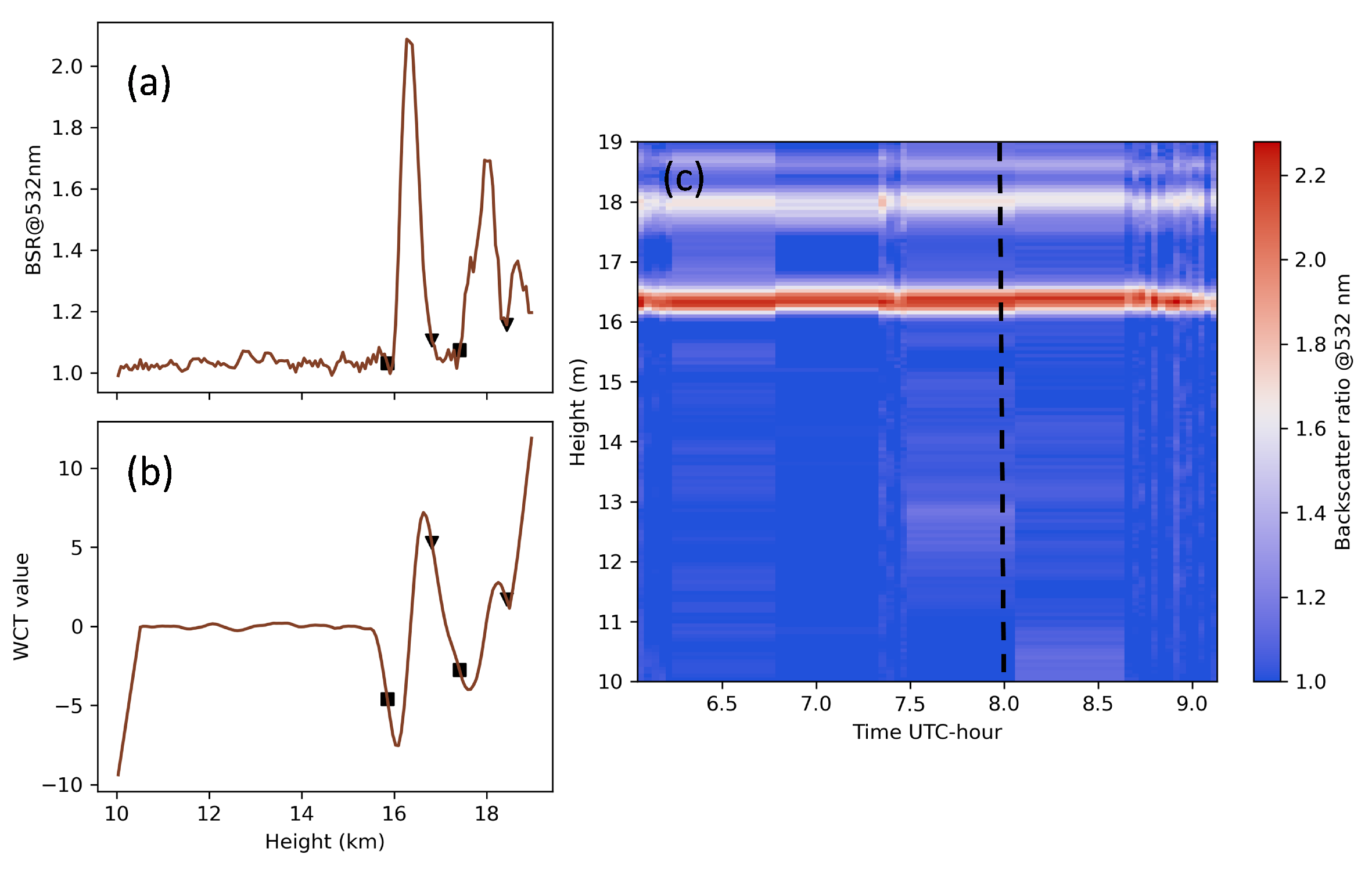
Appendix B. Example of WCT Method Applied to Two Layers of Cirrus Clouds

Figure A2 gives an example of this method in 6 December 2018. There are two distinct layers of cirrus as shown in Figure A2c by the enhancement of BSR from the clear sky background BSR equal to unity. In Figure A2a,b, these two lower and higher layers detected by the WCT method are shown.
Figure A2. An example case for the WCT method: (a) BSR at 532 nm and (b) WCT value as a function of height in 8:00 UTC. The squares show the height of the cloud base and the triangles show the height of the cloud top detected by the WCT method. (c) BSR at 532 nm as a function of time and height measured by lidar on 6 December 2018. The dashed line shows the time in 8:00 UTC.
Remotesensing 16 01448 g0a2

Appendix C. Sensitivity Study for the Multiple Scattering Effect

Here, we give an example case to show the MS effect and why we can neglect it under most circumstances. Figure A3 shows the increase in lidar signal. The strength of this signal shows the fraction of the MS light compared to the single scattered light. If the cloud COD is below 0.1, no MS occurs. Here, the plot shows a noise of around ±2% as the conditions above the cloud may not be perfectly uniform, or the impact of noise in the lidar system is too large. If the cloud COD increases to values around 0.3, the MS increases the lidar signal by about 5%. This means that the impact of MS is below or equal to 5% and therefore negligible. If the COD increases to values of around 2, the MS is something like 9% and if the cloud becomes even thicker, the lidar beam will no longer penetrate. This is also not the case we consider, as the COD of cirrus over Palau is generally low and rarely greater than 1.0 (see Figure 10).
Figure A3. The increase in the lidar signal as a function of COD between 10.8 and 16.8 km on 2 September 2022; with 600 s temporal resolution, there are 25-time steps for analysis, and the latter 3-time steps have a cloud are so thick that the lidar signal is noise and was screened out based on the scheme as mentioned in the Section 2.3.1. Different colors show two examples for low COD (<1) and high COD about 2.
Remotesensing 16 01448 g0a3

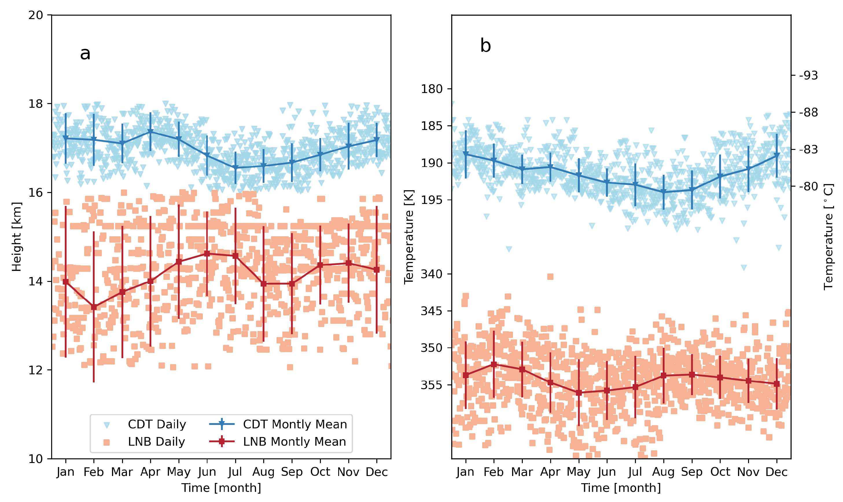
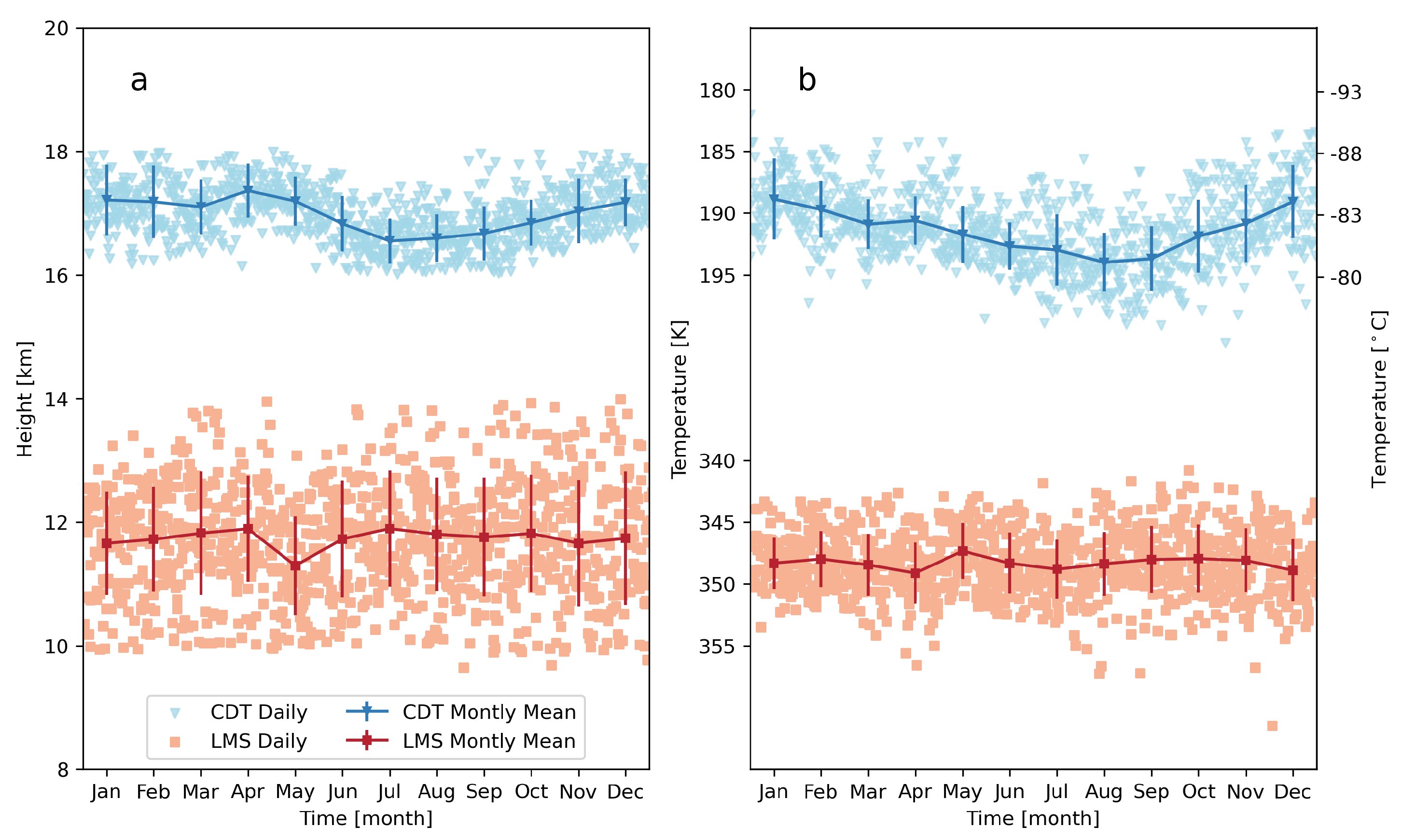
Appendix D. The TTL Features over Palau

Many studies, e.g., [8,69,70,71], have been performed and focused on the physical and chemical processes of the TTL, and different upper and lower boundaries are taken into consideration because of the different central points of these studies. The feature of TTL over Palau is shown in Figure A4 and Figure A5. The lower limit of the TTL is the Level of Main Convective Outflow (LMCO) which is also the Level of Neutral Buoyancy (LNB) at around 14–15 km. Additionally, the level of minimum stability (LMS) [72] or the lapse rate minimum (LRM) [73] typically around 10–12 km, is also important and associated with cloud base height in certain months such as April and May, see Section 3.1 and Figure 6.
Figure A4. Daily and monthly averaged (a) height (km) and (b) temperature (K) of cold point tropopause (CPT, red) and level of neutral buoyancy (LNB, blue) in 2018, 2019, and 2022 for each day (not only for the day lidar was operating). Note that the y axis of (b) for LNB is the potential temperature (K) and the double y axis is for CPT in different units: K and °C. The monthly mean and with 1- σ standard error of the data are shown by a red line and error bar, respectively. Daily data are shown by the square triangle and square for CDT and LNB, respectively. The meteorology profiles are from radio soundings by the National Weather Service of Palau, see Section 2.2.2.
Remotesensing 16 01448 g0a4
Figure A5. Similar plot of Figure A4 but for cold point tropopause (CPT, red) and the level of minimum stability (LMS, blue).
Remotesensing 16 01448 g0a5
The level of the Cold Point Tropopause (CPT), which is the level of temperature minimum [73,74] or the Lapse Rate Tropopause (LRT; World Meteorological Organization, 1957), is used to identify the upper TTL, which is about 17 km. Fueglistaler et al. [8] proposed a Level of Highest Convective Overshooting (LHCO) tops that can reach about 18.5 km (70 hPa) as the upper limit of the TTL. Previous studies have demonstrated, using radio soundings [75,76] and cirrus cloud observations [9,12], that there is a maximum static stability layer [77] within 2 km of thickness above the conventional top of the thermal troposphere (CPT/LRT). In this layer, the trace gases such as O3 and CO also show a large vertical gradient [78,79], which implies the need for a higher upper limit of the TTL as the air eventually transits into the lower stratosphere. Even though this is the most concise definition incorporating most previous research on this topic [80,81], the exact level of LHCO is difficult to quantify compared with the thermal tropopause CPT/LRT, and varies in different places and seasons. Thus, this study will use the CPT definition to give a picture of the upper TTL region above Palau, as can be seen in Section 3.4.
The lowest height is around 16 km and the highest temperature is around 195 K of CPT, which occurs in the summer from July to August in Palau. In winter, the coldest CPT temperature approaches 185 k in December, January, and February. This specific lowermost temperature of CPT is important for the dehydration process of the optically thin cirrus in TWP. It can be seen that the height and temperature of LMS have no clear seasonal variation compared to CPT but with only one minimum height in May. The height of LMS stays stable at about 11.6 km and a temperature of 347 K. The height of LNB is about 14.5 km with a first maximum from May to July and a second maximum in October and November. The minimum of LNB is in February.

References

  1. Sassen, K.; Wang, Z.; Liu, D. Global distribution of cirrus clouds from CloudSat/Cloud-Aerosol lidar and infrared pathfinder satellite observations (CALIPSO) measurements. J. Geophys. Res. Atmos. 2008, 113. [Google Scholar] [CrossRef]
  2. Sassen, K.; Wang, Z.; Liu, D. Cirrus clouds and deep convection in the tropics: Insights from CALIPSO and CloudSat. J. Geophys. Res. Atmos. 2009, 114. [Google Scholar] [CrossRef]
  3. Liou, K.N. Influence of Cirrus Clouds on Weather and Climate Processes: A Global Perspective. Mon. Weather. Rev. 1986, 114, 1167–1199. [Google Scholar] [CrossRef]
  4. Burkhardt, U.; Kärcher, B. Global radiative forcing from contrail cirrus. Nat. Clim. Change 2011, 1, 54–58. [Google Scholar] [CrossRef]
  5. Haladay, T.; Stephens, G. Characteristics of tropical thin cirrus clouds deduced from joint CloudSat and CALIPSO observations. J. Geophys. Res. Atmos. 2009, 114. [Google Scholar] [CrossRef]
  6. Zhou, C.; Dessler, A.E.; Zelinka, M.D.; Yang, P.; Wang, T. Cirrus feedback on interannual climate fluctuations. Geophys. Res. Lett. 2014, 41, 9166–9173. [Google Scholar] [CrossRef]
  7. Fueglistaler, S.; Wernli, H.; Peter, T. Tropical troposphere-to-stratosphere transport inferred from trajectory calculations. J. Geophys. Res. Atmos. 2004, 109. [Google Scholar] [CrossRef]
  8. Fueglistaler, S.; Dessler, A.E.; Dunkerton, T.J.; Folkins, I.; Fu, Q.; Mote, P.W. Tropical tropopause layer. Rev. Geophys. 2009, 47. [Google Scholar] [CrossRef]
  9. Immler, F.; Krüger, K.; Tegtmeier, S.; Fujiwara, M.; Fortuin, P.; Verver, G.; Schrems, O. Cirrus clouds, humidity, and dehydration in the tropical tropopause layer observed at Paramaribo, Suriname (5.8°N, 55.2°W). J. Geophys. Res. Atmos. 2007, 112. [Google Scholar] [CrossRef]
  10. Fu, Q.; Smith, M.; Yang, Q. The Impact of Cloud Radiative Effects on the Tropical Tropopause Layer Temperatures. Atmosphere 2018, 9, 377. [Google Scholar] [CrossRef]
  11. Lynch, D.K. Cirrus: History and Definitions. In Cirrus; Oxford University Press: Oxford, UK, 2002; pp. 11–40. [Google Scholar]
  12. Immler, F.; Krüger, K.; Fujiwara, M.; Verver, G.; Rex, M.; Schrems, O. Correlation between equatorial Kelvin waves and the occurrence of extremely thin ice clouds at the tropical tropopause. Atmos. Chem. Phys. 2008, 8, 4019–4026. [Google Scholar] [CrossRef]
  13. Jensen, E.J.; Thornberry, T.D.; Rollins, A.W.; Ueyama, R.; Pfister, L.; Bui, T.; Diskin, G.S.; DiGangi, J.P.; Hintsa, E.; Gao, R.S.; et al. Physical processes controlling the spatial distributions of relative humidity in the tropical tropopause layer over the Pacific. J. Geophys. Res. Atmos. 2017, 122, 6094–6107. [Google Scholar] [CrossRef]
  14. DeMott, P. Cirrus: Laboratory Studies of Cirrus Cloud Processes; Oxford University Press: Oxford, UK, 2002; pp. 102–135. [Google Scholar]
  15. Krämer, M.; Rolf, C.; Luebke, A.; Afchine, A.; Spelten, N.; Costa, A.; Meyer, J.; Zöger, M.; Smith, J.; Herman, R.L.; et al. A microphysics guide to cirrus clouds – Part 1: Cirrus types. Atmos. Chem. Phys. 2016, 16, 3463–3483. [Google Scholar] [CrossRef]
  16. Pfister, L.; Selkirk, H.B.; Jensen, E.J.; Schoeberl, M.R.; Toon, O.B.; Browell, E.V.; Grant, W.B.; Gary, B.; Mahoney, M.J.; Bui, T.V.; et al. Aircraft observations of thin cirrus clouds near the tropical tropopause. J. Geophys. Res. Atmos. 2001, 106, 9765–9786. [Google Scholar] [CrossRef]
  17. Comstock, J.M.; Jakob, C. Evaluation of tropical cirrus cloud properties derived from ECMWF model output and ground based measurements over Nauru Island. Geophys. Res. Lett. 2004, 31. [Google Scholar] [CrossRef]
  18. Waliser, D.E.; Gautier, C. A Satellite-derived Climatology of the ITCZ. J. Clim. 1993, 6, 2162–2174. [Google Scholar] [CrossRef]
  19. Sun, X.; Palm, M.; Müller, K.; Hachmeister, J.; Notholt, J. Determination of the chemical equator from GEOS-Chem model simulation: A focus on the tropical western Pacific region. Atmos. Chem. Phys. 2023, 23, 7075–7090. [Google Scholar] [CrossRef]
  20. Holton, J.R.; Gettelman, A. Horizontal transport and the dehydration of the stratosphere. Geophys. Res. Lett. 2001, 28, 2799–2802. [Google Scholar] [CrossRef]
  21. Jensen, E.J.; Toon, O.B.; Pfister, L.; Selkirk, H.B. Dehydration of the upper troposphere and lower stratosphere by subvisible cirrus clouds near the tropical tropopause. Geophys. Res. Lett. 1996, 23, 825–828. [Google Scholar] [CrossRef]
  22. Fujiwara, M.; Iwasaki, S.; Shimizu, A.; Inai, Y.; Shiotani, M.; Hasebe, F.; Matsui, I.; Sugimoto, N.; Okamoto, H.; Nishi, N.; et al. Cirrus observations in the tropical tropopause layer over the western Pacific. J. Geophys. Res. Atmos. 2009, 114. [Google Scholar] [CrossRef]
  23. Jensen, E.J.; Smith, J.B.; Pfister, L.; Pittman, J.V.; Weinstock, E.M.; Sayres, D.S.; Herman, R.L.; Troy, R.F.; Rosenlof, K.; Thompson, T.L.; et al. Ice supersaturations exceeding 100% at the cold tropical tropopause: Implications for cirrus formation and dehydration. Atmos. Chem. Phys. 2005, 5, 851–862. [Google Scholar] [CrossRef]
  24. Schoeberl, M.R.; Jensen, E.J.; Pfister, L.; Ueyama, R.; Wang, T.; Selkirk, H.; Avery, M.; Thornberry, T.; Dessler, A.E. Water Vapor, Clouds, and Saturation in the Tropical Tropopause Layer. J. Geophys. Res. Atmos. 2019, 124, 3984–4003. [Google Scholar] [CrossRef] [PubMed]
  25. Sassen, K.; Cho, B.S. Subvisual-Thin Cirrus Lidar Dataset for Satellite Verification and Climatological Research. J. Appl. Meteorol. Climatol. 1992, 31, 1275–1285. [Google Scholar] [CrossRef]
  26. McFarquhar, G.M.; Heymsfield, A.J.; Spinhirne, J.; Hart, B. Thin and Subvisual Tropopause Tropical Cirrus: Observations and Radiative Impacts. J. Atmos. Sci. 2000, 57, 1841–1853. [Google Scholar] [CrossRef]
  27. Heymsfield, A.J. Ice Particles Observed in a Cirriform Cloud at −83 °C and Implications for Polar Stratospheric Clouds. J. Atmos. Sci. 1986, 43, 851–855. [Google Scholar] [CrossRef]
  28. Reverdy, M.; Noel, V.; Chepfer, H.; Legras, B. On the origin of subvisible cirrus clouds in the tropical upper troposphere. Atmos. Chem. Phys. 2012, 12, 12081–12101. [Google Scholar] [CrossRef]
  29. Holton, J.R.; Haynes, P.H.; McIntyre, M.E.; Douglass, A.R.; Rood, R.B.; Pfister, L. Stratosphere-troposphere exchange. Rev. Geophys. 1995, 33, 403–439. [Google Scholar] [CrossRef]
  30. Platt, C.M.R.; Scott, S.C.; Dilley, A.C. Remote Sounding of High Clouds. Part VI: Optical Properties of Midlatitude and Tropical Cirrus. J. Atmos. Sci. 1987, 44, 729–747. [Google Scholar] [CrossRef]
  31. Platt, C.M.R.; Young, S.A.; Manson, P.J.; Patterson, G.R.; Marsden, S.C.; Austin, R.T.; Churnside, J.H. The Optical Properties of Equatorial Cirrus from Observations in the ARM Pilot Radiation Observation Experiment. J. Atmos. Sci. 1998, 55, 1977–1996. [Google Scholar] [CrossRef]
  32. Sassen, K.; Benson, S. A Midlatitude Cirrus Cloud Climatology from the Facility for Atmospheric Remote Sensing. Part II: Microphysical Properties Derived from Lidar Depolarization. J. Atmos. Sci. 2001, 58, 2103–2112. [Google Scholar] [CrossRef]
  33. Pace, G.; Cacciani, M.; di Sarra, A.; Fiocco, G.; Fuà, D. Lidar observations of equatorial cirrus clouds at Mahé Seychelles. J. Geophys. Res. Atmos. 2003, 108. [Google Scholar] [CrossRef]
  34. Das, S.K.; Chiang, C.W.; Nee, J.B. Characteristics of cirrus clouds and its radiative properties based on lidar observation over Chung-Li, Taiwan. Atmos. Res. 2009, 93, 723–735. [Google Scholar] [CrossRef]
  35. Pandit, A.K.; Gadhavi, H.; Ratnam, M.V.; Jayaraman, A.; Raghunath, K.; Rao, S.V.B. Characteristics of cirrus clouds and tropical tropopause layer: Seasonal variation and long-term trends. J. Atmos. Sol. Terr. Phys. 2014, 121, 248–256. [Google Scholar] [CrossRef]
  36. Stephens, G.L.; Vane, D.G.; Boain, R.J.; Mace, G.G.; Sassen, K.; Wang, Z.; Illingworth, A.J.; O’Connor, E.J.; Rossow, W.B.; Durden, S.L.; et al. THE CLOUDSAT MISSION AND THE A-TRAIN: A New Dimension of Space-Based Observations of Clouds and Precipitation. Bull. Am. Meteorol. Soc. 2002, 83, 1771–1790. [Google Scholar] [CrossRef]
  37. Pandit, A.K.; Gadhavi, H.S.; Venkat Ratnam, M.; Raghunath, K.; Rao, S.V.B.; Jayaraman, A. Long-term trend analysis and climatology of tropical cirrus clouds using 16 years of lidar data set over Southern India. Atmos. Chem. Phys. 2015, 15, 13833–13848. [Google Scholar] [CrossRef]
  38. Cairo, F.; De Muro, M.; Snels, M.; Di Liberto, L.; Bucci, S.; Legras, B.; Kottayil, A.; Scoccione, A.; Ghisu, S. Lidar observations of cirrus clouds in Palau (7°N, 134°E). Atmos. Chem. Phys. 2021, 21, 7947–7961. [Google Scholar] [CrossRef]
  39. Müller, K.; Tradowsky, J.S.; von der Gathen, P.; Ritter, C.; Patris, S.; Notholt, J.; Rex, M. Measurement report: The Palau Atmospheric Observatory and its ozonesonde record—continuous monitoring of tropospheric composition and dynamics in the tropical western Pacific. Atmos. Chem. Phys. 2024, 24, 2169–2193. [Google Scholar] [CrossRef]
  40. Müller, K. Characterization of Ozone and the Oxidizing Capacity of the Tropical West Pacific Troposphere. Ph.D. Thesis, Fachbereich Physik und Elektrotechnik der Universität, Bremen, Germany, 2020. [Google Scholar]
  41. Global Modeling and Assimilation Office (GMAO). MERRA-2 tavgU_2d_ocn_Nx: 2d,diurnal, Time-Averaged, Single-Level, Assimilation, Ocean Surface Diagnostics, V5.12.4; Goddard Earth Sciences Data and Information Services Center (GES DISC): Greenbelt, MD, USA, 2015. [Google Scholar] [CrossRef]
  42. Immler, F.; Beninga, I.; Ruhe, W.; Stein, B.; Mielke, B.; Rutz, S.; Terli, O.; Schrems, O. A new LIDAR system for the detection of Cloud and aerosol backscatter, depolarization, extinction, and fluorescence. In Proceedings of the 23rd International Laser Radar Converence, Nara, Japan, 24–28 July 2006; Nagasawa, C., Sugimoto, N.I., Eds.; National Center for Atmospheric Research, Earth Observing Laboratory: Boulder, CO, USA, 2006; pp. 35–38. [Google Scholar]
  43. Dirksen, R.; Sommer, M.; Immler, F.; Hurst, D.; Kivi, R.; Vömel, H. Reference quality upper-air measurements: GRUAN data processing for the Vaisala RS92 radiosonde. Atmos. Meas. Tech. 2014, 7, 4463–4490. [Google Scholar] [CrossRef]
  44. Sun, B.; Reale, T.; Schroeder, S.; Pettey, M.; Smith, R. On the accuracy of Vaisala RS41 versus RS92 upper-air temperature observations. J. Atmos. Ocean. Technol. 2019, 36, 635–653. [Google Scholar] [CrossRef]
  45. Bucholtz, A. Rayleigh-scattering calculations for the terrestrial atmosphere. Appl. Opt. 1995, 34, 2765–2773. [Google Scholar] [CrossRef]
  46. Klett, J.D. Lidar inversion with variable backscatter/extinction ratios. Appl. Opt. 1985, 24, 1638–1643. [Google Scholar] [CrossRef] [PubMed]
  47. Nakoudi, K.; Stachlewska, I.S.; Ritter, C. An extended lidar-based cirrus cloud retrieval scheme: First application over an Arctic site. Opt. Express 2021, 29, 8553–8580. [Google Scholar] [CrossRef] [PubMed]
  48. Ritter, C.; Neuber, R.; Schulz, A.; Markowicz, K.; Stachlewska, I.; Lisok, J.; Makuch, P.; Pakszys, P.; Markuszewski, P.; Rozwadowska, A.; et al. 2014 iAREA campaign on aerosol in Spitsbergen—Part 2: Optical properties from Raman-lidar and in situ observations at Ny-Ålesund. Atmos. Environ. 2016, 141, 1–19. [Google Scholar] [CrossRef]
  49. Ångström, A. On the atmospheric transmission of sun radiation and on dust in the air. Geogr. Ann. 1929, 11, 156–166. [Google Scholar]
  50. Dionisi, D.; Keckhut, P.; Liberti, G.L.; Cardillo, F.; Congeduti, F. Midlatitude cirrus classification at Rome Tor Vergata through a multichannel Raman–Mie–Rayleigh lidar. Atmos. Chem. Phys. 2013, 13, 11853–11868. [Google Scholar] [CrossRef]
  51. Baars, H.; Ansmann, A.; Engelmann, R.; Althausen, D. Continuous monitoring of the boundary-layer top with lidar. Atmos. Chem. Phys. 2008, 8, 7281–7296. [Google Scholar] [CrossRef]
  52. Nakoudi, K.; Ritter, C.; Stachlewska, I.S. Properties of Cirrus Clouds over the European Arctic (Ny-Ålesund, Svalbard). Remote Sens. 2021, 13, 4555. [Google Scholar] [CrossRef]
  53. Voudouri, K.A.; Giannakaki, E.; Komppula, M.; Balis, D. Variability in cirrus cloud properties using a PollyXT Raman lidar over high and tropical latitudes. Atmos. Chem. Phys. 2020, 20, 4427–4444. [Google Scholar] [CrossRef]
  54. Burton, S.; Ferrare, R.; Vaughan, M.; Omar, A.; Rogers, R.; Hostetler, C.; Hair, J. Aerosol classification from airborne HSRL and comparisons with the CALIPSO vertical feature mask. Atmos. Meas. Tech. 2013, 6, 1397–1412. [Google Scholar] [CrossRef]
  55. Giannakaki, E.; Balis, D.; Amiridis, V.; Kazadzis, S. Optical and geometrical characteristics of cirrus clouds over a Southern European lidar station. Atmos. Chem. Phys. 2007, 7, 5519–5530. [Google Scholar] [CrossRef]
  56. Hogan, R.J. Fast approximate calculation of multiply scattered lidar returns. Appl. Opt. 2006, 45, 5984–5992. [Google Scholar] [CrossRef]
  57. Eloranta, E.W. Practical model for the calculation of multiply scattered lidar returns. Appl. Opt. 1998, 37, 2464–2472. [Google Scholar] [CrossRef]
  58. Sun, X.; Ritter, C.; Mueller, K. ACCLIP: ComCAL Raman Lidar Data, Version 1.0; UCAR/NCAR—Earth Observing Laboratory: Boulder, CO, USA, 2023. [CrossRef]
  59. Seifert, P.; Ansmann, A.; Müller, D.; Wandinger, U.; Althausen, D.; Heymsfield, A.J.; Massie, S.T.; Schmitt, C. Cirrus optical properties observed with lidar, radiosonde, and satellite over the tropical Indian Ocean during the aerosol-polluted northeast and clean maritime southwest monsoon. J. Geophys. Res. Atmos. 2007, 112. [Google Scholar] [CrossRef]
  60. Gouveia, D.A.; Barja, B.; Barbosa, H.M.J.; Seifert, P.; Baars, H.; Pauliquevis, T.; Artaxo, P. Optical and geometrical properties of cirrus clouds in Amazonia derived from 1 year of ground-based lidar measurements. Atmos. Chem. Phys. 2017, 17, 3619–3636. [Google Scholar] [CrossRef]
  61. Martins, E.; Noel, V.; Chepfer, H. Properties of cirrus and subvisible cirrus from nighttime Cloud-Aerosol Lidar with Orthogonal Polarization (CALIOP), related to atmospheric dynamics and water vapor. J. Geophys. Res. Atmos. 2011, 116. [Google Scholar] [CrossRef]
  62. Virts, K.S.; Wallace, J.M. Observations of Temperature, Wind, Cirrus, and Trace Gases in the Tropical Tropopause Transition Layer during the MJO. J. Atmos. Sci. 2014, 71, 1143–1157. [Google Scholar] [CrossRef]
  63. Virts, K.S.; Wallace, J.M.; Fu, Q.; Ackerman, T.P. Tropical tropopause transition layer cirrus as represented by CALIPSO lidar observations. J. Atmos. Sci. 2010, 67, 3113–3129. [Google Scholar] [CrossRef]
  64. Müller, K.; Wohltmann, I.; von der Gathen, P.; Rex, M. Air Mass Transport to the Tropical West Pacific Troposphere inferred from Ozone and Relative Humidity Balloon Observations above Palau. EGUsphere 2023, 2023, 1–37. [Google Scholar] [CrossRef]
  65. Flury, T.; Wu, D.L.; Read, W.G. Correlation among cirrus ice content, water vapor and temperature in the TTL as observed by CALIPSO and Aura/MLS. Atmos. Chem. Phys. 2012, 12, 683–691. [Google Scholar] [CrossRef]
  66. Zou, L.; Griessbach, S.; Hoffmann, L.; Gong, B.; Wang, L. Revisiting global satellite observations of stratospheric cirrus clouds. Atmos. Chem. Phys. 2020, 20, 9939–9959. [Google Scholar] [CrossRef]
  67. Jensen, E.J.; Pfister, L.; Bui, T.P.; Lawson, P.; Baumgardner, D. Ice nucleation and cloud microphysical properties in tropical tropopause layer cirrus. Atmos. Chem. Phys. 2010, 10, 1369–1384. [Google Scholar] [CrossRef]
  68. Rex, M.; Wohltmann, I.; Ridder, T.; Lehmann, R.; Rosenlof, K.; Wennberg, P.; Weisenstein, D.; Notholt, J.; Krüger, K.; Mohr, V.; et al. A tropical West Pacific OH minimum and implications for stratospheric composition. Atmos. Chem. Phys. 2014, 14, 4827–4841. [Google Scholar] [CrossRef]
  69. Gettelman, A.; Birner, T.; Eyring, V.; Akiyoshi, H.; Bekki, S.; Brühl, C.; Dameris, M.; Kinnison, D.E.; Lefevre, F.; Lott, F.; et al. The Tropical Tropopause Layer 1960–2100. Atmos. Chem. Phys. 2009, 9, 1621–1637. [Google Scholar] [CrossRef]
  70. Gettelman, A.; Forster, P.M.d.F.; Fujiwara, M.; Fu, Q.; Vömel, H.; Gohar, L.K.; Johanson, C.; Ammerman, M. Radiation balance of the tropical tropopause layer. J. Geophys. Res. Atmos. 2004, 109. [Google Scholar] [CrossRef]
  71. Folkins, I.; Loewenstein, M.; Podolske, J.; Oltmans, S.J.; Proffitt, M. A barrier to vertical mixing at 14 km in the tropics: Evidence from ozonesondes and aircraft measurements. J. Geophys. Res. Atmos. 1999, 104, 22095–22102. [Google Scholar] [CrossRef]
  72. Sunilkumar, S.; Muhsin, M.; Venkat Ratnam, M.; Parameswaran, K.; Krishna Murthy, B.; Emmanuel, M. Boundaries of tropical tropopause layer (TTL): A new perspective based on thermal and stability profiles. J. Geophys. Res. Atmos. 2017, 122, 741–754. [Google Scholar] [CrossRef]
  73. Gettelman, A.; de Forster, P.M. A climatology of the tropical tropopause layer. J. Meteorol. Soc. Jpn. Ser. II 2002, 80, 911–924. [Google Scholar] [CrossRef]
  74. Highwood, E.; Hoskins, B. The tropical tropopause. Q. J. R. Meteorol. Soc. 1998, 124, 1579–1604. [Google Scholar] [CrossRef]
  75. Gettelman, A.; Wang, T. Structural diagnostics of the tropopause inversion layer and its evolution. J. Geophys. Res. Atmos. 2015, 120, 46–62. [Google Scholar] [CrossRef]
  76. Birner, T.; Sankey, D.; Shepherd, T.G. The tropopause inversion layer in models and analyses. Geophys. Res. Lett. 2006, 33. [Google Scholar] [CrossRef]
  77. Pilch Kedzierski, R.; Matthes, K.; Bumke, K. The tropical tropopause inversion layer: Variability and modulation by equatorial waves. Atmos. Chem. Phys. 2016, 16, 11617–11633. [Google Scholar] [CrossRef]
  78. Schmidt, T.; Cammas, J.P.; Smit, H.G.J.; Heise, S.; Wickert, J.; Haser, A. Observational characteristics of the tropopause inversion layer derived from CHAMP/GRACE radio occultations and MOZAIC aircraft data. J. Geophys. Res. Atmos. 2010, 115. [Google Scholar] [CrossRef]
  79. Park, S.; Jiménez, R.; Daube, B.C.; Pfister, L.; Conway, T.J.; Gottlieb, E.W.; Chow, V.Y.; Curran, D.J.; Matross, D.M.; Bright, A.; et al. The CO2 tracer clock for the Tropical Tropopause Layer. Atmos. Chem. Phys. 2007, 7, 3989–4000. [Google Scholar] [CrossRef]
  80. Sun, X. The Atmospheric Transport in the Western Pacific Region by Measurements and Model Simulations. Ph.D. Thesis, Fachbereich Physik und Elektrotechnik der Universität, Bremen, Germany, 2024. [Google Scholar] [CrossRef]
  81. Henz, D.R. A Modeling Study of the Tropical Tropopause Layer. Master’s Thesis, University of Wisconsin, Madison, WI, USA, 2010. [Google Scholar]
Figure 1. Maps of the location of Koror, Palau. (a) The site is located in Koror (marked on the left side of the map), the main commercial center of the Republic of Palau, an island country in the Micronesia subregion of Oceania in the western Pacific. (b) Sea Surface temperature (SST, in °C) in the tropical region averaged from 2015 to 2022. The black line shows the isothermal line of 28.5 °C. The location of Palau is marked in the plot. The SST data are obtained from the ocean surface diagnostic data collection in Modern-Era Retrospective Analysis for Research and Applications version 2 (MERRA-2) [41].
Remotesensing 16 01448 g001
Figure 2. (a) Schematic diagram of the ComCAL system. (b) The laser and top part of the lab container of the Palau Atmospheric Observatory (PAO) during the night. (c) Laser window. (d) Parabolic mirror with 400 mm aperture and 1200 mm focal length. (e) Picture of the ComCAL system inside the lab container.
Remotesensing 16 01448 g002
Figure 3. (a) Schematic diagram and (b) photo of the detector optics: 1: 90° off-axis mirror, 2, 3, 4, 7: dichroic mirrors, 5: detector for 1064 nm signal (interference filter, lens, APD), 6: rotating Glan–Taylor prism, 8, 9: Detectors for 532 nm and 355 nm signals (interference filters, lens, PMT), 10: Detector for 387 nm signal (interference filter, lens, PMT).
Remotesensing 16 01448 g003
Figure 4. Height–time plot of backscatter ratio (BSR) at 532 nm with cirrus cloud base C b a s e (blue dots) and top C t o p (orange dots) derived by the wavelet covariance transform (WCT) method. Lidar observations using ComCAL over Koror, Palau on (a) 5 August 2022, (b) 25 August 2022, and (c) 17 August 2022, represent three different scenarios of cloud geometric thickness ranging from thick to thin.
Remotesensing 16 01448 g004
Figure 5. Schematic of the data processing used by the ComCAL to obtain cirrus properties.
Remotesensing 16 01448 g005
Figure 6. Cirrus monthly percentage occurrence (PO) in Palau by ComCAL. The numbers in Figure 6 refer to the detected cirrus layers. The blue and orange square with 1- σ shows the height of the cloud base and the top of the cloud base. The height of cold point tropopause (CPT, brown circles), level of neutral buoyancy (LNB, pink “X”s), and level of the minimum stability (LMS, cyan triangles) averaged each month was calculated by the meteorology profiles from radiosondes by the National Weather Service of Palau. See details of CPT and LMS in the Appendix D. The monthly occurrence of cirrus clouds is calculated from the data solely collected within each month of the year, as shown by the x ticks.
Remotesensing 16 01448 g006
Figure 7. Percentage occurrence (PO) of cirrus in Palau during winter (December–February, red line), spring (March–May, yellow line), summer (July–August, green line), Autumn (October–November, brown line), and yearly averaged (dashed black line). The annual mean of the cold point tropopause (CPT gray dashed line), the level of neutral buoyancy (LNB, dotted line), and the level of minimum stability (LMS, dotted dashed line) are shown. For the specific months, years and seasonal divisions of the dataset, please see Table 1.
Remotesensing 16 01448 g007
Figure 8. Frequency of occurrence (FOC) distributions of the seasonal and annual geometrical thickness (GT) of cloud (ae), C b a s e (fj) and C t o p (ko). The bin size is 1 km. It should be noted that the FOC values add up to 1.0, and for the sake of aesthetics of the picture, only the maximum value of FOC is displayed in the y axis of this figure, so the vertical coordinate of the picture is less than 1.0.
Remotesensing 16 01448 g008
Figure 9. FOC distributions of the seasonal and annual cloud base temperature (ae), cloud top temperature (fj), and mid-cloud temperature (ko). The bin size is 5 °C.
Remotesensing 16 01448 g009
Figure 10. FOC distributions of the seasonal and annual COD (ae) particle depolarization ratio (fg) and color ratio (ko). The bin size for (ae) is 0.2, for (fj) is 0.1 and for (fj) is 0.25.
Remotesensing 16 01448 g010
Figure 11. (a) Annual averaged FOC distribution of the cloud base height with different CODs as indicated by different colors and markers. The dashed line shows the distribution of the height of the CPT. (b) FOC of seasonal and annual ETTCi*, SVC, thin, and thick cloud. Since the FOC of ETTCi is very low compared to several other types of clouds, it is difficult to see its exact frequency of occurrence in the figure; please see Table 3 for details of its value. Note that ETTCi [9] is a customized sub-classification of cirrus with a COD defined as less than 0.005, which belongs to SVC. The sum of the fraction of SVC, thin, and thick cirrus equals 1.0, which should not include the fraction of ETTCi.
Remotesensing 16 01448 g011
Figure 12. (a) Time series of the daily averaged mid-cloud height of sub-visible cirrus (SVC, shown by green triangles), extremely thin tropical cirrus (ETTCi, shown by black “X”s) and cold point tropopause (CPT, shown by black circles). (b) Time series of the distance from the cold point tropopause (CPT) to the daily averaged mid-cloud height of SVC and ETTCi cirrus cloud. If the distance is a negative value, the cloud layer is higher than the CPT, and vice versa.
Remotesensing 16 01448 g012
Table 1. Year, month and seasonal division of lidar observations.
YearMonthSeason
2018DecemberWinter
2018January
2019February
2022MarchSpring
2018April
2018May
2022JulySummer
2022August
2018OctoberAutumn
2018November
Table 2. Specifications of the detector channels.
Channel (nm)Pulse Energy (mJ)Max. Transmission
106412082%
53218036%
3556552%
Table 3. Seasonal and annual mean and standard deviation statistics for cirrus geometrical and optical properties.
Cirrus PropertiesAnnualWinterSpringSummerAutumn
Cloud base temperature (°C)−71.7 ± 11.5−73.7 ± 10.9−67.9 ± 12.5−63.4 ± 13.6−64.5 ± 13.4
Cloud top temperature (°C)−75.9 ± 9.0−82.5 ± 4.8−71.9 ± 10.1−76.4 ± 6.8−73.9 ± 11.4
Mid-cloud temperature (°C)−70.4 ± 10.4−78.1 ± 7.1−67.9 ± 10.8−69.9 ± 9.0−69.0 ± 12.0
Geometrical thickness (km)1.5 ± 0.91.6 ± 0.91.0 ± 0.51.9 ± 1.21.4 ± 0.7
Cloud base height (km)14.1 ± 1.715.3 ± 1.414.0 ± 1.713.9 ± 1.814.0 ± 1.7
Cloud top height (km)15.8± 1.416.9 ± 1.015.1 ± 1.615.8 ± 1.215.4 ± 1.6
COD0.25 ± 0.450.17 ± 0.330.15 ± 0.300.33 ± 0.530.19 ± 0.35
ETTCi */SVC/thin/thick (%)1.6/32/46/226.2/39/47/142.0/46/43/110.7/28/43/290.6/32/54/14
Color ratio (355/532)1.6 ± 0.51.5 ± 0.51.6 ± 0.41.1 ± 0.11.6 ± 0.5
LDPR (%)31 ± 1934 ± 2225 ± 1636 ± 1824 ± 16
* ETCCi [9] is a sub-classification of cirrus with a COD less than 0.005, which belongs to SVC. The sum of the fraction of SVC, thin, and thick cirrus equals 1.0, which should not include the fraction of ETTCi.
Table 4. Statistics for the cirrus properties based on lidar measurements at different tropical sites.
Site C base (km) C top (km)GT (km)Temperature (°C)Reference
Koror
(7.3°N, 134.5°E)
14.1 ± 1.715.8 ± 1.41.5 ± 0.9−74 ± 10this study
Gwal Pahari
(28.43°N, 77.15°E)
9.0 ± 1.510.6 ± 1.81.5 ± 0.7−33 ± 6[53]
Elandsfontein
(26.25°S, 29.43°E)
9.2 ± 0.810.8 ± 0.91.6 ± 0.7−34 ± 5
Chung-Li
(24.58°N, 121.10°E)
12.3 ± 2.214.4 ± 1.71.5 ± 0.7-[34]
Gadanki
(13.5°N, 79.2°E)
13.0 ± 2.215.3 ± 2.02.3 ± 1.3−65 ± 12[35]
Hulule
(4.1°N, 73.3°E)
11.9 ± 1.613.7 ± 1.41.8 ± 1.0−58 ± 11[59]
Amazonia
(2.9°S, 59.9°W)
12.9 ± 2.214.3 ± 1.91.4 ± 1.1−60 ± 15[60]
Nauru Island
(0.5°S, 166.9°E)
-16.5–17.0--[17]
Tropics ± 30° *-14.3 ± 1.70.6 ± 0.2−66 ± 10[61]
* Based on Cloud-Aerosol Lidar with Orthogonal Polarization (CALIOP) [36] spaceborne lidar observations.
Disclaimer/Publisher’s Note: The statements, opinions and data contained in all publications are solely those of the individual author(s) and contributor(s) and not of MDPI and/or the editor(s). MDPI and/or the editor(s) disclaim responsibility for any injury to people or property resulting from any ideas, methods, instructions or products referred to in the content.

