


Bridging Domains and Resolutions: Deep Learning-Based Land Cover Mapping without Matched Labels

1
Research Center of Forestry Remote Sensing & Information Engineering, Central South University of Forestry & Technology, Changsha 410004, China
2
Hunan Provincial Key Laboratory of Forestry Remote Sensing Based Big Data & Ecological Security, Changsha 410004, China
3
Key Laboratory of National Forestry and Grassland Administration on Forest Resources Management and Monitoring in Southern China, Changsha 410004, China
4
School of Civil Engineering, Sun Yat-sen University, Zhuhai 519082, China
*
Author to whom correspondence should be addressed.
Remote Sens. 2024, 16(8), 1449; https://doi.org/10.3390/rs16081449
Submission received: 21 February 2024
/
Revised: 12 April 2024
/
Accepted: 17 April 2024
/
Published: 19 April 2024
(This article belongs to the Special Issue New Deep Learning Paradigms for Multisource Remote Sensing Data Fusion and Classification)
Abstract
:High-resolution land cover mapping is crucial in various disciplines but is often hindered by the lack of accurately matched labels. Our study introduces an innovative deep learning methodology for effective land cover mapping, independent of matched labels. The approach comprises three main components: (1) An advanced fully convolutional neural network, augmented with super-resolution features, to refine labels; (2) The application of an instance-batch normalization network (IBN), leveraging these enhanced labels from the source domain, to generate 2-m resolution land cover maps for test sites in the target domain; (3) Noise assessment tests to evaluate the impact of varying noise levels on the model’s mapping accuracy using external labels. The model achieved an overall accuracy of 83.40% in the target domain using endogenous super-resolution labels. In contrast, employing exogenous, high-precision labels from the National Land Cover Database in the source domain led to a notable accuracy increase of 2.55%, reaching 85.48%. This improvement highlights the model’s enhanced generalizability and performance during domain shifts, attributed significantly to the IBN layer. Our findings reveal that, despite the absence of native high-precision labels, the utilization of high-quality external labels can substantially benefit the development of precise land cover mapping, underscoring their potential in scenarios with unmatched labels.
1. Introduction
Land cover mapping plays an instrumental role in depicting the Earth’s surface characteristics, essential for environmental monitoring and management [1,2]. The dynamic interplay of policy shifts and natural events continuously alters land cover, necessitating regular updates to maintain the credibility of these maps [3,4].
Historically, land cover mapping relied heavily on manual delineation, a process fraught with inefficiencies [5]. The integration of computers, geographic information systems, and remote sensing technologies has revolutionized this field, leading to the development of automated methods, with machine learning emerging as a crucial component [6]. Deep learning, a more recent advancement in this domain, has surpassed traditional machine learning methods in classification accuracy [7]. However, deep learning’s effectiveness is contingent on the availability of large, annotated datasets that can be both costly and labor-intensive [8]. For instance, in the U.S., a Chesapeake Bay watershed’s land cover map was produced with costly labels (USD 1.3 million over 10 months) [9]. The current trend in land cover mapping utilizes existing land cover products as training labels [10,11], a practice supported by the availability of various global-scale products, including FROM-GLC30 [12], Globaland30 [13], ESA WorldCover [14], and so on. However, these products are limited by their resolution, typically ranging from 10 m to 30 m, and are influenced by the data sources, classification techniques, and scales.
Now, there is a growing demand for high-resolution (HR) land cover mapping [15]. Some studies have attempted to improve the resolution of these labels using techniques like up-sampling [16] (i.e., the nearest neighbor method [17]), but this approach often introduces significant noise, compromising the quality of the resulting maps [18]. In response, researchers have explored label super-resolution (SR) using deep learning, aiming to generate HR land cover maps from low-resolution (LR) labels. For instance, Malkin et al. [19] introduced an innovative SR loss function along with a fully convolutional neural network (FCN) that effectively generate a 1-m resolution land cover map. Nevertheless with LR labels, HR labels remains indispensable for the realization of this approach. Li et al. [20] developed an SR loss function that utilizes 30-m low-resolution labels to produce 1-m resolution maps, further advancing this field. However, these methods face challenges due to the inherent inaccuracies in LR labels and the noise introduced by the resolution disparity, affecting the final mapping quality.
Global land cover datasets also exhibit inconsistencies in accuracy and spatial congruity, influenced by varying classification techniques, data collection timelines, and sensor types. For instance, the ESRI 2020 Global Land Use Land Cover dataset asserts an accuracy of 85%, while ESA reports a precision of about 75% [14,21]. And the ESRI product’s overall accuracy in China is now at 64%, whereas that of the ESA product hovers around 67% [22]. Furthermore, classification accuracy can significantly differ even within the same dataset, such as the FROM-GLC 30 dataset, with user accuracy for grassland and shrubland at merely 38.13% and 39.04%, respectively [12]. Consequently, the reliability of utilizing these publicly available global land cover datasets for land cover mapping directly remains open to debate.
Compared to global products, certain publicly accessible national-scale land cover products display a better level of accuracy. For instance, within the U.S. region, the National Land Cover Database (NLCD) with a resolution of 30 m shows an overall accuracy of approximately 83.1% [23], which has become fundamental in various applications related to land cover within the U.S. [24]. However, these datasets are confined solely to the U.S. Considering the temporal, spatial, and thematic discrepancies, models trained on national-scale data encounter limitations when it comes to being direct applied to different regions [25]. To address such challenges, domain shift methodologies are commonly employed, such as maximum mean discrepancy (MMD) [26] and generative adversarial networks (GANs) [27]. Among them, the Instance-Batch Normalization Network (IBN-Net) [28], a network focused on domain shift, effectively mitigates the effects of seasonal land cover changes, light effects, and internal grade variations on domain shift [29].
The challenge of achieving precise, high-resolution land cover mapping is exacerbated by the limited availability of detailed labels. Within this context, the utilization of pre-existing LR land cover products to facilitate HR land cover mapping constitutes a challenging yet auspicious venture. Malkin et al. [30] used epitomic representations and a label SR algorithm to create HR land cover maps of the northern U.S. using LR data from the southern U.S. However, this methodology exclusively navigated domain shift within the confines of the U.S. Comparatively, prior scholarly exploration has understudied the amalgamation of label SR and domain shift, thereby presenting a relatively uncharted enigma. Research on domain shift has laid the groundwork for integrating data from different regions, yet the combination of label SR and domain shift remains a relatively unexplored territory. This synergy could potentially overcome regional variations in precision and the limitations of LR labels in deep learning.
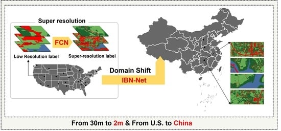
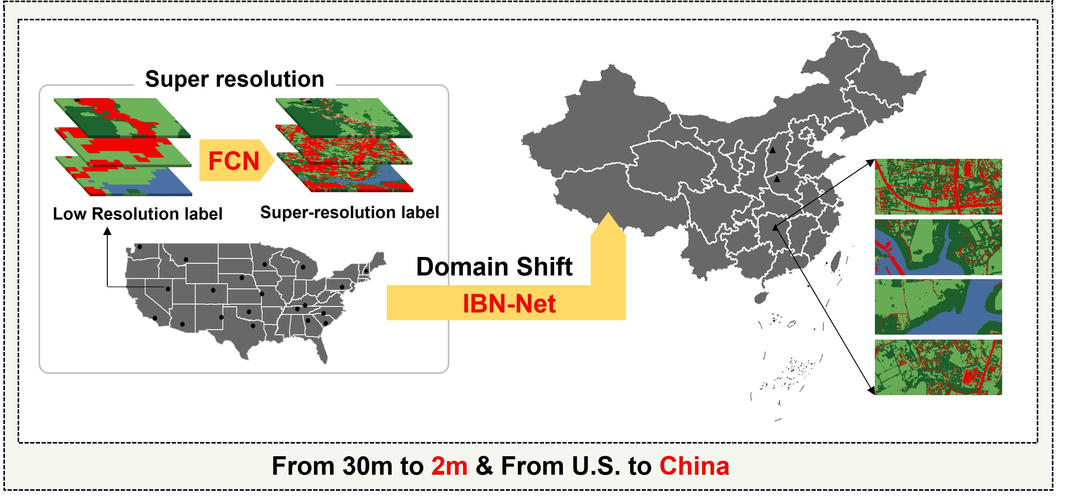
To address these challenges, this study introduces a novel approach for enhancing land cover mapping accuracy without matched labels. This novel methodology encompasses the integration of FCN for SR and IBN-Net for land cover mapping, capitalizing on HR Google Earth imagery and LR land cover products from the source domain. As a result, it yields finely detailed 2-m resolution land cover maps for the target domain without matching labels. The overall procedure of this study is depicted in Figure 1.
2. Materials and Methods
2.1. Study Area and Dataset
2.1.1. Data Acquisition
In this research, the United States and China were selected as the source and target domains, respectively. The study involved the selection of sample points across 23 distinct regions within each domain. These regions comprised three non-overlapping testing zones specifically designated for precision assessment, in addition to 20 training sample areas. These samples collectively encompass an estimated land area of 262,202.05 km2, encompassing a diverse range of landscapes. The spatial arrangement of these sample points in both the source and target domains is visually represented in Figure 2. In support of our experimental endeavors, we acquired several key datasets, as detailed in Table 1. While NLCD pertains to national-scale data, covering only the source domain, we procured the other global products for both the target and source domains. To ensure synchronization in a temporal context with the labeled data, 2.04-m Google Earth images for the respective time periods were obtained.
2.1.2. Reclassification
Five distinct land cover datasets were utilized in this experiment. To standardize the classification criteria and enhance the validation of the proposed methodology, a reclassification of sample labels was imperative. Owing to the absence of ice and snow across the chosen sample points, this specific land type is excluded from consideration. By harmonizing the label taxonomy, these classifications of all land cover products are amalgamated, culminating in the formation of four ultimate classes: water (W), low vegetation (LV), impervious surface (I), and forest (F). The detailed classification criteria are delineated in Table 2.
2.1.3. Preprocessing of Dataset
Bilinear interpolation resampling [31] was employed, by which LR labels underwent resampling to 2 m and were subsequently reprojected onto the WGS84 coordinate system, ensuring conformity with the Google Earth imagery. Utilizing a sliding window approach with a 0.2 overlap, both imagery and labels underwent cropping to generate an aligned dataset (4000 × 4000). To guarantee dataset quality, image tiles of subpar quality (with missing data, imaging abnormalities, and excessive cloud cover) were filtered out.
All processing was implemented using Python 3.9. Ultimately, for each of the five labels, this iterative process resulted in a total of 1442 training pairs for the target domain and 1994 training pairs for the source domain, respectively. The training pairs were further divided into training and validation sets, in a 9:1 ratio, respectively, used for training the model and determining the hyperparameters, as discussed in Section 2.2.1 and Section 2.2.2. An isolated extraction of 20% of the training pairs was manually re-annotated for accuracy assessment in Section 3.1. And the optimal land cover dataset generated in Section 2.2.1 was subsequently used to serve as training data for Section 2.2.2. For the testing region, the same approach as described above was employed, with the only difference being that the size of the testing images was 256 × 256. Ultimately, a total of 8020 and 8308 testing images were obtained from the test sites in the source and target domains, respectively, which were solely utilized for the evaluation (Section 3.2) of the model from Section 2.2.2. More details are shown in Table 3. In Section 2.2.2, the Maryland HR land cover map (https://planning.maryland.gov/Pages/OurWork/landuse.aspx) was utilized as supplementary data for assisting in the calculation of the loss function parameters; it was similarly cropped to a size of 4000 × 4000 to align with the LR label.
2.2. Methodology
2.2.1. Label Super-Resolution
Both the HR image and LR label are georeferenced, facilitating the calculation of the geospatial correspondences between the individual LR pixel and the numerous HR prediction pixels (Figure 3b). Consequently, the label SR method is contingent upon a distribution shared between the LR class categories and the more detailed HR land cover classes.
Due to the mosaic and LR nature of land cover datasets, there exists a risk of overfitting noisy labels when employing advanced networks featuring large receptive fields or encoder–decoder structures. To mitigate this concern, we adopt the FCN with a small receptive field as the core segmentation model for label SR [32]. The encoding process commences with the input image traversing five feature extraction layers. This involves the utilization of a stack containing 64 filters of 3 × 3 convolutions, along with ReLU and max-pooling layers. Subsequently, a classification layer employs a 1 × 1 convolution to predict scores corresponding to each class. To enrich the contextual information extraction from images, tile-by-tile algorithms are seamlessly integrated into the network [30] (Figure 3a). Ultimately, the network’s output feature map undergoes processing by the loss function.
The loss function proposed by [19] is referenced in this work. is utilized to define the LR labeling, while corresponds to the HR labeling. For a given LR label, k, the conjoint distribution is established. This distribution describes the frequency distribution of the HR class labels, denoted as n, within an LR block labeled as k (Figure 3c). The parameters governing this distribution are deduced from the Maryland HR land cover product [19] for the source and target domains. These parameters encompass both the label frequencies (), the anticipated percentage () for each target land cover class, and the associated standard deviation (). The probabilistic outcome of the core segmentation model, , is envisaged as the independent generation of labels for individual HR pixels within an HR input image. These labels are then aggregated through a label-counting layer module. To gauge the disparity between the two distributions, a statistics matching module is employed. This module quantifies the mismatch between the generated probabilistic labels and the labels derived from the conjoint distribution, D(, ). This disparity acts as an optimization criterion to enhance the core segmentation model’s performance, wherein the Kullback–Leibler (KL) divergence is employed to quantify the evaluation of the matching process (Figure 3c), that is
2.2.2. IBN-Net
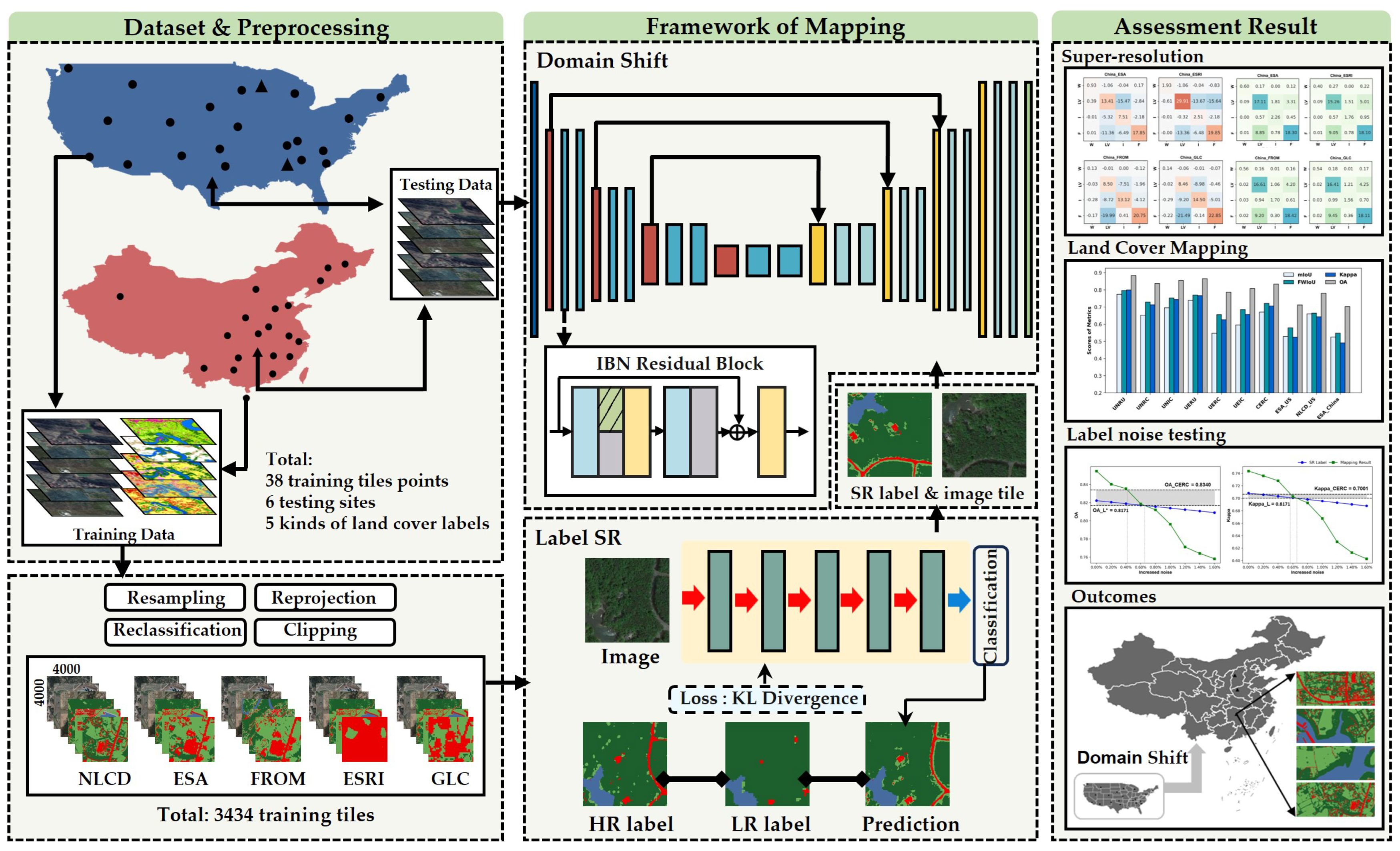
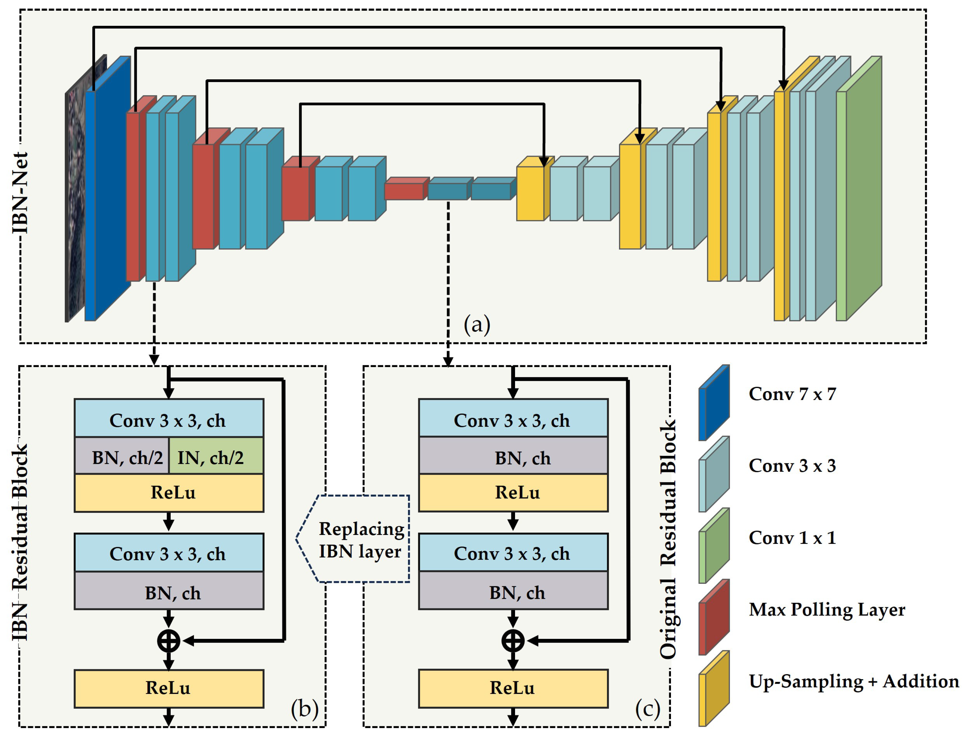
A discernible disparity in visual land features exists between the landscapes of the source and target domains. To effectively gain the precise land cover mapping in the target domain using labels from the source domain, an improved instance-batch normalization network (IBN-Net) was meticulously devised. The foundational model adopts the U-Net architecture, enriched with the ResNet-18 encode. This framework encompasses a foundational backbone network tasked with feature extraction, a bottleneck layer housing a pair of convolutional strata supplemented by dropout functionality, and a classifier engineered to forecast a coarse segmentation outcome from the highest-level feature stratum. Symmetry is maintained in both the encoding and decoding processes, bolstered by skip connections. The encoder module employs the ResNet-18 framework with four clusters of residual blocks, all dedicated to extracting salient features. Within each residual block, a sequence of two 3 × 3 convolutions is trailed by a ReLU activation function. Subsequently, the output undergoes up-sampling. The incorporation of a shortcut mechanism via ResNet-18 serves the dual purpose of mitigating gradient vanishing issues and expediting network convergence. In the decoder phase, the original U-Net decoding architecture is embraced (Figure 4a).
Applying an instance normalization (IN) module enhances the performance of the residual block (Figure 4b,c). The process involves segmenting the output of the convolutional layer and subsequently employing batch normalization (BN) for half of the channels, while the remaining channels undergo IN application after the initial convolutional layer. Following the separate calculation of the IN and BN layers, their outputs are amalgamated. Within the IN layer, normalization is executed on the mean and standard deviation of the RGB channels, serving to alleviate intricate variations in appearance. This results in improved visual and appearance invariance. The IN procedure utilizes individual sample statistics to normalize features, maintaining uniformity between training and inference processes. Conversely, BN, designed to preserve texture-related features, is commonly leveraged in image classification and semantic segmentation tasks. Furthermore, BN normalizes input data for each layer, lessening the scale disparity among the input characteristic values. This, in turn, magnifies the network’s gradient and mitigates the issue of gradient vanishing. Notably, shallow neural networks focus on surface-level attributes, while deeper counterparts convey richer semantic information [29]. To selectively retain a portion of the BN features, effectively reducing feature variance induced by appearance disparities in shallow layers, and simultaneously safeguarding content discrimination in deep layers, IN layers are exclusively added to the first three groups (conv2x-conv4x). The fourth group (conv5x) remains untouched to maintain its original configuration.
The loss function used by the model is the cross-entropy loss [33]. Assuming n is the total number of categories (), and i represents the category (). For each pixel, the loss function is defined as follows:
where is the loss value, is the value of class i in the true labels, and is the probability of class i in the model’s output.
2.3. Implementation Details
The proposed method was implemented in PyTorch 1.8 on a GeForce RTX 3080 GPU. The AdamW optimizer was applied for training. In the training process of label SR, every tile, where each includes 4000 × 4000 pixels, was randomly cropped into 100 patches with the size of 256 × 256. After obtaining the SR labels, the aligned dataset of 4000 × 4000 HR tiles was cropped into non-overlapping patches of size 256 × 256 as input for IBN-Net. The detailed parameters of the model are presented in Table 4 and the specific details regarding the involvement of different types of data from various land cover datasets have been elaborated in Section 2.1.3.
2.4. Comparison Methods
In the label SR section, a comparative evaluation was initially conducted on various land cover products to identify the optimal LR and SR labels (SR-B), which were than used in Section 2.2.2 and Section 3.2. This section not only compares the accuracy of the original LR land cover data across the source and target domains but also evaluates the changes in accuracy of the land cover data following label SR processing, as well as the differences between various SR datasets.
The land cover mapping section encompasses seven control group comparison methods designed to validate the performance of land cover mapping from SR endogenous (labels from the target area) and exogenous (labels from other areas) labels, along with a comparative analysis between domain-shift and non-domain-shift outcomes. Furthermore, a baseline assessment is conducted using an unmodified Resnet18-UNet. To ensure a fair evaluation, the configuration of these models adheres to the guidelines elucidated in Section 2.3. A comprehensive overview of the comparative experimental design and the explanation of abbreviations corresponding to the experiments are provided in Table 5.
2.5. Evaluation Metrics
This study utilizes established quantitative metrics for a comprehensive assessment of the research findings [34]. These metrics encompass the mean intersection over union (mIoU), the frequency-weighted intersection over union (FWIoU), the Kappa coefficient, and the overall accuracy (OA). Among these metrics, mIoU is a metric that evaluates the average overlap between predicted and actual target areas, providing insight into the model’s precision in spatial segmentation tasks. FWIoU enhances the mIoU by incorporating class frequency into the calculation, thereby giving more weight to more common classes and ensuring a balanced evaluation across varied class distributions. The Kappa coefficient measures the agreement between two sets of categorical data, accounting for the possibility of the agreement occurring by chance, which offers a robust indicator of the model’s classification accuracy beyond mere chance. Lastly, OA quantifies the proportion of correctly predicted observations to the total observations, offering a straightforward metric of the model’s performance across all categories.
For the datasets related to the source and target domains, 20% of the training and testing pairs were manually annotated. These annotated pairs are utilized as the ground truth for assessing the accuracy of label super-resolution and for the final evaluation of land cover prediction.
Assuming n is the total number of categories (), and i represents the category (). Define , , , and as representing true positives, true negatives, false positives, and false negatives, respectively. . The calculation formulas and descriptions are as follows:
3. Results and Analysis
3.1. Super Resolution
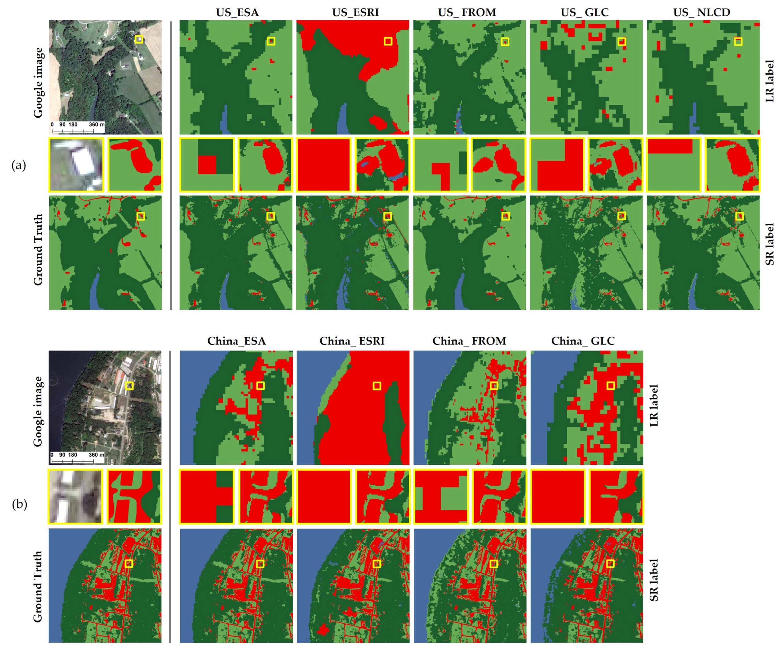
To assess the quantitative impact attributed to labeling errors and instances of category confusion within LR labels, as well as to gauge the enhancements brought about by SR, a confusion matrices comparison for the LR labels was undertaken (Figure 5a,b). Confusion between the forest and low vegetation categories occurs most frequently, with an average of . The improved matrix (Figure 5c) and visual result (Figure 6) demonstrates a substantial improvement in the classification accuracy of the classes following the application of label SR. This is due to the small receptive field of FCN for label SR, which successfully reduces the negative impacts of spatial blurring seen in the coarse labels. Notably, there are noteworthy increments observed in the detection of TP for both the forest and low vegetation categories, accompanied by corresponding reductions in FP and false negatives FN for these classes.
The IoU scores and OA for virtually all classes show improvement after label SR (Figure 7). The quality of various land cover products varies. The NLCD stands out as the label with the highest OA, while the ESA product emerges as the global product showcasing the optimal quality for the target region. While the presence of LR label noise is commonly observed at the edges, the substantial noise within the original LR labels due to factors such as resolution and mapping techniques hinders the clear differentiation of closely related land cover classes. Consequently, the application of these products with more noise proves unsuitable for the precise delineation of intricate land cover nuances. Subsequent land cover mapping will incorporate labels from US_NLCD, US_ESA, and China_ESA.
Figure 5.
Confusion matrices before and after label SR. (a) is the comparing confusion matrices for different land cover products before and after SR in source domain. (b) is comparing confusion matrices for different land cover products before and after SR in target domain. (c) is the improved confusion matrices after label SR depicting the transformation from LR label to SR. For (a,b), values on the diagonal represent the number of pixels that are correctly labeled. The improved matrix is obtained by subtracting (a) from (b).

Figure 6.
Visualized results of labeled SR. (a) is the visual comparison for different land cover products before and after SR in source domain; (b) is the visual comparison for different land cover products before and after SR in target domain.
Figure 6.
Visualized results of labeled SR. (a) is the visual comparison for different land cover products before and after SR in source domain; (b) is the visual comparison for different land cover products before and after SR in target domain.

Figure 7.
OA and IoU scores of each category for different labels. (a) shows the OA of LR and SR labels; (b) shows the IoU score of LR and SR labels in various land cover categories.
Figure 7.
OA and IoU scores of each category for different labels. (a) shows the OA of LR and SR labels; (b) shows the IoU score of LR and SR labels in various land cover categories.

3.2. Land Cover Mapping
Divergent land cover characteristics and distributions distinguish the source and target domains. To assess the efficacy of the proposed approach across diverse scenarios, a comprehensive comparative analysis, encompassing both visual and statistical aspects, was conducted.
3.2.1. Visualization and Qualitative Analysis
In order to provide a visualization comparison, typical land cover scenarios from the target domain and the source domain are presented in Figure 8 and Figure 9.
In Figure 8a–h and Figure 9a–t, the predicted outcomes derived from the model incorporating ESA labels are characterized by a noticeable coarseness and errors. In Figure 9i,j,m,n, there is an imprecise and intermittent recognition of continuous water boundaries. This could potentially be attributed to the images of water exhibiting characteristics similar to water vegetation. Consequently, in the LR ESA product, a substantial portion of W is classified as either LV or F, thus culminating in the subsequent misclassification of W through similar spectral imaging by models with ESA labels. The model with NLCD labels demonstrates a heightened degree of precision in the extraction of water body boundaries. Concurrently, all the experimental findings concur in unveiling the presence of varying levels of incongruous noise related to low vegetation. Furthermore, of note is the proximity of impervious surfaces derived from UNRU and UNIC to the ground truth. Notably, the capacity for detecting features of diminutive buildings within the LR product proves to be consistently subpar. However, a discernible improvement is observable within LR NLCD, where a multitude of modest structures situated within urban landscapes, alongside the foliage encompassing these buildings, are classified as impervious surfaces [35]. Consequently, this phenomenon enhances the efficacy of impervious surface mapping.
In comparison to land cover mapping within the source domain, the models employing SR NLCD and ESA data from the source domain yielded unsatisfactory outcomes when applied to the target domain directly, as evident in Figure 9a–d,i–l, among which, UERC exhibits its most pronounced shortcomings across various scenarios. Notably, disparities in land cover attributes between the target and source domains emerged, encompassing not only surface imaging characteristics, such as texture, color, and size of ground cover entities, but also the spatial distribution pattern of the ground cover [36]. The direct transfer of model frameworks trained on the source domain labels to the target domain revealed that, although models like UNRC produced results exhibiting precise boundaries, their performance remained lackluster concerning intricate land cover categories. This discrepancy culminated in predictions suffering from incongruous noise and a lack of fitting.
UNIC and UEIC, utilize labels originating from the source domain, the singular divergence of which lies in the presence of IBN layers within the model architecture. Specifically, scenarios 1 and 2 encompass a diverse array of dense structural formations, wherein diminutive edifices interlace with shrubbery and the canopies of trees. Within the subplots of Figure 9b,n, instances arise where shadows around the building are incorrectly identified as I class. In Figure 9a,i,j, the erroneous classification of roads and structures adjacent to them is apparent, with incorrect allocation to alternative land cover categories. In contrast to this, UNIC and UEIC, incorporating the IBN layer, demonstrate an augmented capacity for generalization, yielding a heightened efficacy in recognizing diverse land cover features and preserving a more intricate spectrum of land cover nuances.
Despite LR China_ESA exhibiting lower accuracy compared to LR US_ESA, the mapping effect of CEIC exceeds that of UEIC and UERC. After incorporating the IBN module, CEIC witnessed an improvement in the result, but it demonstrates limited efficacy in scenarios involving intricate land cover classes (e.g., Figure 9r,t fail to identify buildings and roads). Even CEIC with local labels (Figure 9e–h) does not overshadow the superiority exhibited by UNIC in qualitative comparisons.
3.2.2. Quantitative Analysis
For quantitative comparison, the computation of all metrics was predicated upon the HR ground references. To fortify the reliability of our comparative analysis, we present the IoU score heatmaps corresponding to distinct methods in Figure 10. After this, Figure 6 and Figure 11 juxtapose the mIoU, FWIoU, Kappa, and OA scores across all methods in all test sites.
As depicted in Figure 10, the classification of forest yields consistently favorable outcomes, with IoU values surpassing 0.7 in nearly all experiments. This trend may be attributed to the substantial availability of training samples for the forest category. In contrast, the performances of the “water” and “impervious surface” classes are markedly subpar. Within these categories, the IoU scores exhibit a comparatively limited range, spanning from 0.41 to 0.63 for water and from 0.46 to 0.64 for impervious surfaces, respectively.
The IoU scores from distinct experiments also exhibit variations in the classification of diverse land cover categories. During the execution of land cover classification within identical geographical extents, the IoU score trends of the experimental outcomes harmonize predominantly with those of the LR labels (Figure 7). Specifically, the IoU scores for each classification category within models with NLCD_US surpass those with ESA_US. Across varying geographical zones, even with the same labels, the IoU scores for individual classes deviate. It is evident that beyond the influence of training data on the efficacy of land cover classification, the attributes and distinguishability of the ground entities within the target area also exert an impact on the performance of mapping. In terms of overall performance, a balanced and robust outcome is observed in the case of UNRU and UNIC. This outcome stands out when juxtaposed with the alternative comparison methods used in both the source and target domains.
In the context of the Chinese testing data experiment, the inclusion of the IBN layer (from UNRC to UNIC, and from UERC to UEIC) yields a notable enhancement in the accuracy of all categories. Particularly noteworthy is the substantial advancement in the water class, demonstrating an average accuracy increase of 8% in comparison to models lacking the IBN layer. Nonetheless, discerning between related land cover classes remains a challenge, attributable to the exacerbation of label noise. This phenomenon compounds the adverse effect on the classification of analogous ground entities for UEIC [34].
While LR ESA_US exhibits superior IOU scores compared to LR ESA_China in the categories of impervious surface and forest, the effectiveness of the trained models (UERC and UEIC) in extracting each land cover type within the target domain falls short of that achieved by the model trained using Chinese local labels (CEIC). When applied within the target domain using NLCD labels, UNRC’s performance surpasses that of CEIC in the forest category but yields less favorable results in the remaining classes. Upon integration with the IBN layer (UNIC), the scores across all classes generally surpass those of CEIC, with the forest class achieving an IOU score of up to 0.8.
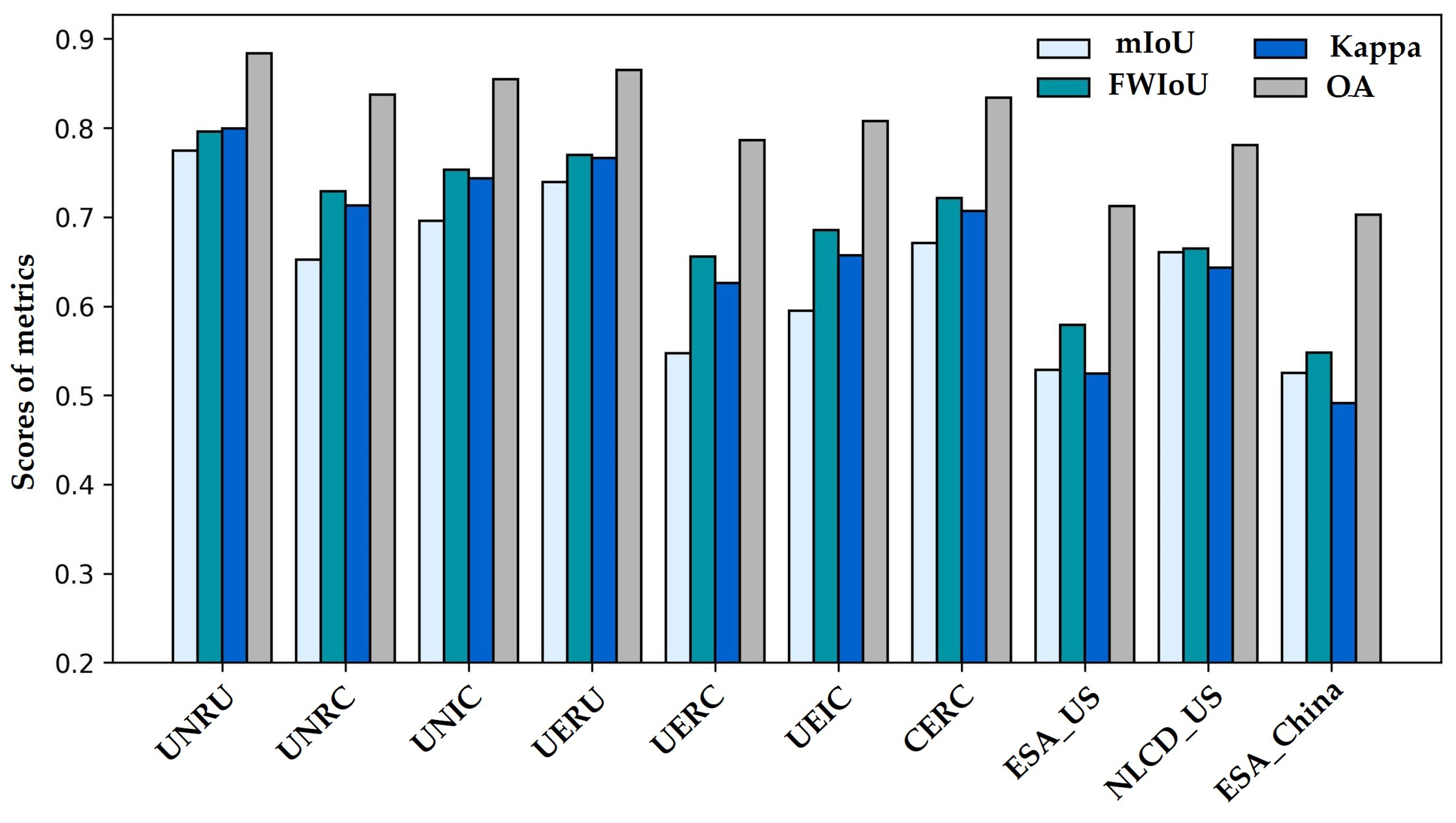
Through analysis of both Table 6 and Figure 11, a comprehensive evaluation of the metrics insensitive (mIoU and OA) and sensitive (FWIoU and Kappa) to category proportion reveals that the comparison methods yield closely aligned quantitative outcomes across distinct test plots. UERC exhibits the least favorable performance, exhibiting average FWIoU and Kappa values of 0.66 and 0.63, respectively, followed by UEIC. And UERC more closely approaches that of the LR labels. It is noteworthy that for land cover mapping in the target and source domains, models utilizing NLCD_US manifest the most favorable results across all metrics.
Due to the intricate architecture of the network, there may be excessive down-sampling. This, in turn, fosters congruence between predictions and the overarching coarse labels. However, it proves unsuitable for effectively capturing the intricate nuances of fine-grained land cover features, especially when dealing with a substantial volume of inaccurately annotated samples. Consequently, when employing an identical model, distinct labels yield disparate outcomes. Upon replacing the labels from the noise-laden ESA with the less noisy NLCD, a notable enhancement is observed, with the FWIoU and Kappa values exhibiting improvements ranging from 2.59% to 7.34% and 3.28% to 8.72%, respectively. However, compared with the noise caused by ESA_China, the dissimilarities in the visual characteristics of ground objects between the target and source domains exert a profound influence on the outcomes. Consequently, the performance of the model trained on ESA_US data is inferior when compared with CEIC. In comparison to CNRC, UNRC showcases slightly reduced IoU scores (0.59 and 0.56, respectively) for the water and impervious surface categories. Nonetheless, their FWIoU, Kappa, and OA scores surpass those of CNRC due to the relatively minor extent of the water and impervious surface categories within the region.
While convolutional neural networks possess a certain generalization capability, they encounter limitations in classification for images from distinct regions. In contrast, IBN-Net demonstrates superior generalization and enhanced capacity. The incorporation of the IBN layer into UNRC (from UNRC to UNIC) yields a remarkable enhancement, with an augmentation of 2.43–9.78% in FWIoU and 3.04–11.76% in Kappa. When contrasted with CEIC utilizing local labels, UNIC attains an average MIoU of approximately 0.6961 and an OA of 0.8548. For both the MIoU and OA metrics, this denotes enhancements of approximately 2.55% and 2.08%, respectively. Despite observable dissimilarities between the training and test datasets in terms of appearance, the models exhibit enhanced robustness towards appearance variations.
Summarizing from the qualitative and quantitative analyses, it is apparent that the effectiveness of methods employing noisy ESA labels is notably reduced. This leads to the production of mapping results marked by less distinct boundaries and the exclusion of intricate details. In contrast, models utilizing NLCD labels yield mapping outcomes with more accurate boundary delineation. Moreover, the incorporation of the IBN layer into the model bolsters its generalization capabilities, ultimately leading to improved precision in delimiting result boundaries.
4. Discussion
4.1. Comparison of Global Products
We present a subset of test regions within the target domain, encompassing diverse landscapes, such as rivers, buildings, forests, and farmlands. This presentation aims to illustrate the effectiveness of our proposed methodology in land cover mapping and to enable a comparative analysis with established global land cover mapping products, specifically, ESA WorldCover, FROM_GLC100, ESRI_LULC, and GLC_FCS. Upon examination of Figure 12, it becomes evident that our method consistently demonstrates robust and precise mapping capabilities across varied environments while enhancing resolution. Particularly noteworthy is the clear delineation of dense concentrations of buildings, along with improved fidelity in larger land cover categories, such as forests and croplands. Additionally, finer structures are accurately delineated, highlighting the significant advancements resulting from the combined use of label super-resolution and domain adaptation.
In the Introduction section, we highlighted that various factors influence the varying accuracies of different global land cover products across different regions. Particularly concerning our target domain (China), many land cover products exhibit lower accuracies, an assertion validated in Section 3.1 as well. By juxtaposing the results from the method proposed in this paper with global land cover products, it becomes evident that when the accuracy and resolution of global products fail to meet the need for finer land cover information, utilizing higher-accuracy products from other regions as reference labels can facilitate the generation of superior land cover maps.
4.2. Exogenous Label Noise Testing
The outcomes of our experiments highlight the potential for enhanced performance through the utilization of exogenous labels in model training. However, it is crucial to acknowledge that not all exogenous labels yield such benefits. Variations in image texture characteristics arise due to diverse factors, such as vegetation types, architectural styles, lighting conditions, and remote sensing image acquisition across different regions. Moreover, the texture features learned by deep learning models significantly impact their applicability within target areas. Consequently, under comparable levels of accuracy, outcomes derived from endogenous labels consistently outperform those from exogenous labels. Therefore, only exogenous labels attaining a certain level of accuracy with low noise have promise as training labels for domain shift.
In this section, to further investigate the impact of label noise and accuracy on domain shift with exogenous labels, different levels and types of noise were introduced to SR US_NLCD labels to assess the performance of the UNIC. Specifically, the noise was added at proportions ranging from 0.2% to 1.6%, relative to the TP of SR NLCD_US, and this noise augmentation was repeated across eight trials. The locations for introducing simulated label noise were randomly selected. For distinct classes, their corresponding confusion matrix columns, as outlined in Section 3.1, were employed to derive the likelihood of misclassification concerning other categories. This probability computation determined how noise was injected into each class. For instance, pixels initially classified as impervious surfaces were more likely to be mislabeled as low vegetation than as other classes.
Figure 13 illustrates the evaluation metrics of SR labels following noise augmentation, along with the land cover mapping achieved by models trained using exogenous labels with varying degrees of noise. With increase in the proportion of noise, both the accuracy of SR labels and the mapping performance of UNIC experience varying degrees of decline. However, once the noise exceeds 0.42%, the mapping outcomes of models trained with exogenous labels begin to fall behind those with endogenous labels (CEIC). At a noise augmentation level of 0.58%, while falling within the range indicated by the gray region, acceptable graphical outcomes can be achieved. However, all metrics about the proposed method exhibit values lower than those of CEIC. When noise levels escalate beyond 0.66%, the mapping performance experiences a degradation that even surpasses that for exogenous training labels. Under such circumstances, the utilization of coarse exogenous training labels is insufficient to facilitate effective land cover mapping within the target domain.
In conclusion, label noise exerts an influence on the domain shift of deep learning models. The proposed method with exogenous training labels with a low degree of noise can achieve commendable outcomes. When the label noise reaches a certain threshold, it becomes more beneficial to opt for endogenous labels with lower accuracy, as opposed to selecting higher-precision exogenous labels.
4.3. Research Constraints and Opportunities
While this study has yielded significant findings, it is imperative to acknowledge its limitations. The primary constraint lies in the imbalance of the training labels, wherein the distribution of different label categories within the dataset may be uneven. This imbalance has the potential to undermine the model’s performance on certain categories, thereby compromising the accuracy and reliability of the research outcomes. Despite efforts to diversify the sampled scenarios during selection, the issue of class imbalance remains inevitable. Addressing this challenge necessitates targeted adjustments to the dataset or the implementation of other strategies to balance category distributions, thereby enhancing the model’s generalization capability and overall performance. On another note, the methodology proposed in this paper primarily emphasizes a novel approach, with multi-class land cover mapping merely serving as a medium for illustrating this method. For tasks involving semantic segmentation or classification in other domains, the applicability of this method remains pertinent, for instance, for extraction of individual land features, such as forests, water bodies, or buildings. In such tasks targeting specific object classifications, concerns regarding sample balance become less pertinent.
While the domains selected for this study encompass only China and the United States, the methods proposed herein are not confined solely to these regions. Similarly, the applicability of endogenous labels for domain shift extends beyond NLCD. Regarding the target domain chosen for this study, although numerous research teams have previously generated high-resolution land cover maps for local regions within this area, the accuracy and utility of these maps, produced by individual teams, warrant careful consideration when compared to NLCD, a nationally authoritative land cover product. In this context, results generated using existing credible land cover products carry higher credibility. The primary objective of this research is to address the challenge of insufficient matching fine labels, which incur high annotation costs. However, it is worth noting that utilizing existing finely manually annotated labels can also yield effective outcomes for mitigating the lack of labels in the target domain, thus achieving better performance in handling domain shift.
In terms of models, although this study adopts simple models and makes minor modifications only to baseline models (FCN, U-Net, ResNet-18), it is noteworthy that this paper focuses on a novel approach from an unprecedented perspective. Specifically, through the innovative method of selecting higher-precision remote labels as non-algorithmic innovations, it addresses the issue of missing training labels in semantic segmentation. Particularly for tasks with high costs in land cover mapping label production, the proposed method in this paper offers a new approach to improving mapping effectiveness for such tasks. From another perspective, the models chosen in this paper may not be the most effective ones; they serve merely as a means to validate the feasibility of the proposed approach. However, if simple models can achieve the desired results and prove the feasibility of the proposed method, further improvements to the models or selection of better models in the future may yield unexpected benefits.
5. Conclusions
For land cover mapping, achieving highly precise semantic labels through manual interpretation is typically limited to small geographic areas. Consequently, models trained with such labels often lack generalizability when applied to diverse global regions. While global land cover products cover larger spatial scales, they often suffer from varying degrees of label noise. This article presents a novel HR land cover mapping approach utilizing deep learning, thereby eliminating the requirement for precisely matched labels. The methodology involves utilizing FCN for semantic label SR, followed by the application of IBN-Net for land cover mapping using SR labels.
A comprehensive series of experiments conducted on Google Earth images and NLCD datasets demonstrates the pronounced superiority of the proposed method. The outcomes of the land cover mapping experiments reveal that, compared to endogenous labels characterized by higher levels of noise, employing exogenous NLCD labels leads to superior mapping performance within the target domain. This augmentation results in an average OA increase of 2.55%, achieving 85.48%. The diversity between the source and target domains presents challenges for domain shift, while the noise and imprecision of labels significantly impact the SR of labels and interfere with the accuracy of land cover mapping results. This necessitates a choice between utilizing local labels with lower precision or non-local labels with higher precision. Indeed, in the absence of internally generated labels with high precision and the availability of externally annotated data with a certain level of accuracy, the utilization of external annotations proves to be a more advantageous approach for enhancing the accuracy of HR land cover mapping. This helps mitigate the impact of the object appearance gap on mapping to some extent, thereby paving the way for the integration of semantic segmentation models incorporating unmatched labels.
Author Contributions
Conceptualization, S.C. and D.M.; methodology, S.C. and D.M.; software, Y.T.; validation, S.C. and Y.T.; formal analysis, S.C.; investigation, S.C.; resources, S.C.; data curation, S.C.; writing—original draft preparation, S.C.; writing—review and editing, E.Y. and J.J.; visualization, S.C.; supervision, D.M.; project administration, D.M.; funding acquisition, D.M. and E.Y. All authors have read and agreed to the published version of the manuscript.
Funding
This research was funded by the Project Technology Innovation Plan Project of the Hunan Provincial Forestry Department under Grant XLK202108-8, and in part by the National Natural Science Foundation of China under Grant 32071682 and Grant 31901311.
Data Availability Statement
The data presented in this study are available on request from the corresponding author. The data are not publicly available due to confidentiality agreements with participating organizations and the sensitive nature of the information collected, which includes proprietary data and personal identifiable information.
Conflicts of Interest
The authors declare no conflict of interest.
References
- Huang, X.; Yang, D.; He, Y.; Nelson, P.; Low, R.; McBride, S.; Mitchell, J.; Guarraia, M. Land cover mapping via crowdsourced multi-directional views: The more directional views, the better. Int. J. Appl. Earth Obs. Geoinf. 2023, 122, 103382. [Google Scholar] [CrossRef]
- Jiang, J.; Xiang, J.; Yan, E.; Song, Y.; Mo, D. Forest-CD: Forest Change Detection Network Based on VHR Images. IEEE Geosci. Remote Sens. Lett. 2022, 19, 1–5. [Google Scholar] [CrossRef]
- Tong, X.Y.; Xia, G.S.; Zhu, X.X. Enabling country-scale land cover mapping with meter-resolution satellite imagery. ISPRS J. Photogramm. Remote. Sens. 2023, 196, 178–196. [Google Scholar] [CrossRef] [PubMed]
- Paris, C.; Bruzzone, L.; Fernández-Prieto, D. A novel approach to the unsupervised update of land-cover maps by classification of time series of multispectral images. IEEE Trans. Geosci. Remote Sens. 2019, 57, 4259–4277. [Google Scholar] [CrossRef]
- Gaur, S.; Singh, R. A comprehensive review on land use/land cover (LULC) change modeling for urban development: Current status and future prospects. Sustainability 2023, 15, 903. [Google Scholar] [CrossRef]
- Zhao, Z.; Islam, F.; Waseem, L.A.; Tariq, A.; Nawaz, M.; Islam, I.U.; Bibi, T.; Rehman, N.U.; Ahmad, W.; Aslam, R.W.; et al. Comparison of three machine learning algorithms using google earth engine for land use land cover classification. Rangel. Ecol. Manag. 2024, 92, 129–137. [Google Scholar] [CrossRef]
- Feizizadeh, B.; Omarzadeh, D.; Kazemi Garajeh, M.; Lakes, T.; Blaschke, T. Machine learning data-driven approaches for land use/cover mapping and trend analysis using Google Earth Engine. J. Environ. Plan. Manag. 2023, 66, 665–697. [Google Scholar] [CrossRef]
- Kakogeorgiou, I.; Karantzalos, K. Evaluating explainable artificial intelligence methods for multi-label deep learning classification tasks in remote sensing. Int. J. Appl. Earth Obs. Geoinf. 2021, 103, 102520. [Google Scholar] [CrossRef]
- Robinson, C.; Hou, L.; Malkin, K.; Soobitsky, R.; Czawlytko, J.; Dilkina, B.; Jojic, N. Large scale high-resolution land cover mapping with multi-resolution data. In Proceedings of the IEEE/CVF Conference on Computer Vision and Pattern Recognition, Long Beach, CA, USA, 15–20 June 2019; pp. 12726–12735. [Google Scholar]
- Liu, Y.; Zhong, Y.; Ma, A.; Zhao, J.; Zhang, L. Cross-resolution national-scale land-cover mapping based on noisy label learning: A case study of China. Int. J. Appl. Earth Obs. Geoinf. 2023, 118, 103265. [Google Scholar] [CrossRef]
- Li, Z.; Lu, F.; Zhang, H.; Yang, G.; Zhang, L. Change cross-detection based on label improvements and multi-model fusion for multi-temporal remote sensing images. In Proceedings of the 2021 IEEE International Geoscience and Remote Sensing Symposium IGARSS, Brussels, Belgium, 11–16 July 2021; pp. 2054–2057. [Google Scholar]
- Gong, P.; Wang, J.; Yu, L.; Zhao, Y.; Zhao, Y.; Liang, L.; Niu, Z.; Huang, X.; Fu, H.; Liu, S.; et al. Finer resolution observation and monitoring of global land cover: First mapping results with Landsat TM and ETM+ data. Int. J. Remote Sens. 2013, 34, 2607–2654. [Google Scholar] [CrossRef]
- Chen, J.; Chen, J.; Liao, A.; Cao, X.; Chen, L.; Chen, X.; He, C.; Han, G.; Peng, S.; Lu, M.; et al. Global land cover mapping at 30 m resolution: A POK-based operational approach. ISPRS J. Photogramm. Remote Sens. 2015, 103, 7–27. [Google Scholar] [CrossRef]
- Zanaga, D.; Van De Kerchove, R.; Daems, D.; De Keersmaecker, W.; Brockmann, C.; Kirches, G.; Wevers, J.; Cartus, O.; Santoro, M.; Fritz, S.; et al. ESA WorldCover 10 m 2021 v200. Zenodo 2022. [Google Scholar] [CrossRef]
- Mollick, T.; Azam, M.G.; Karim, S. Geospatial-based machine learning techniques for land use and land cover mapping using a high-resolution unmanned aerial vehicle image. Remote. Sens. Appl. Soc. Environ. 2023, 29, 100859. [Google Scholar] [CrossRef]
- Li, R.; Gao, X.; Shi, F.; Zhang, H. Scale Effect of Land Cover Classification from Multi-Resolution Satellite Remote Sensing Data. Sensors 2023, 23, 6136. [Google Scholar] [CrossRef]
- Priscila, S.S.; Rajest, S.S.; Regin, R.; Shynu, T. Classification of Satellite Photographs Utilizing the K-Nearest Neighbor Algorithm. Cent. Asian J. Math. Theory Comput. Sci. 2023, 4, 53–71. [Google Scholar]
- Song, L.; Estes, A.B.; Estes, L.D. A super-ensemble approach to map land cover types with high resolution over data-sparse African savanna landscapes. Int. J. Appl. Earth Obs. Geoinf. 2023, 116, 103152. [Google Scholar] [CrossRef]
- Malkin, K.; Robinson, C.; Hou, L.; Soobitsky, R.; Czawlytko, J.; Samaras, D.; Saltz, J.; Joppa, L.; Jojic, N. Label super-resolution networks. In Proceedings of the International Conference on Learning Representations, Vancouver, BC, Canada, 30 April–3 May 2018. [Google Scholar]
- Li, Z.; Zhang, H.; Lu, F.; Xue, R.; Yang, G.; Zhang, L. Breaking the resolution barrier: A low-to-high network for large-scale high-resolution land-cover mapping using low-resolution labels. ISPRS J. Photogramm. Remote Sens. 2022, 192, 244–267. [Google Scholar] [CrossRef]
- Karra, K.; Kontgis, C.; Statman-Weil, Z.; Mazzariello, J.C.; Mathis, M.; Brumby, S.P. Global land use/land cover with Sentinel 2 and deep learning. In Proceedings of the 2021 IEEE International Geoscience and Remote Sensing Symposium IGARSS, Brussels, Belgium, 11–16 July 2021; pp. 4704–4707. [Google Scholar]
- Kang, J.; Sui, L.; Yang, X.; Wang, Z.; Huang, C.; Wang, J. Spatial pattern consistency among different remote-sensing land cover datasets: A case study in Northern Laos. ISPRS Int. J. Geoinf. 2019, 8, 201. [Google Scholar] [CrossRef]
- Wickham, J.; Stehman, S.V.; Sorenson, D.G.; Gass, L.; Dewitz, J.A. Thematic accuracy assessment of the NLCD 2019 land cover for the conterminous United States. GIsci. Remote Sens. 2023, 60, 2181143. [Google Scholar] [CrossRef]
- Shinskie, J.L.; Delahunty, T.; Pitt, A.L. Fine-scale accuracy assessment of the 2016 National Land Cover Dataset for stream-based wildlife habitat. J. Wildl. Manag. 2023, 87, e22402. [Google Scholar] [CrossRef]
- Bruzzone, L.; Carlin, L. A multilevel context-based system for classification of very high spatial resolution images. IEEE Trans. Geosci. Remote Sens. 2006, 44, 2587–2600. [Google Scholar] [CrossRef]
- Tzeng, E.; Hoffman, J.; Zhang, N.; Saenko, K.; Darrell, T. Deep domain confusion: Maximizing for domain invariance. arXiv 2014, arXiv:1412.3474. [Google Scholar]
- Pan, Z.; Yu, W.; Wang, B.; Xie, H.; Sheng, V.S.; Lei, J.; Kwong, S. Loss functions of generative adversarial networks (GANs): Opportunities and challenges. IEEE Trans. Emerg Top. Comput Intell. 2020, 4, 500–522. [Google Scholar] [CrossRef]
- Pan, X.; Luo, P.; Shi, J.; Tang, X. Two at once: Enhancing learning and generalization capacities via ibn-net. In Proceedings of the European Conference on Computer Vision (ECCV), Munich, Germany, 8–14 September 2018; pp. 464–479. [Google Scholar]
- Pan, X.; Shi, J.; Luo, P.; Wang, X.; Tang, X. Spatial as deep: Spatial cnn for traffic scene understanding. Proc. AAAI Conf. Artif. Intell. 2018, 32, 1. [Google Scholar] [CrossRef]
- Malkin, N.; Ortiz, A.; Jojic, N. Mining self-similarity: Label super-resolution with epitomic representations. In Proceedings of the Computer Vision–ECCV 2020: 16th European Conference, Glasgow, UK, 23–28 August 2020; pp. 531–547. [Google Scholar]
- Smith, P. Bilinear interpolation of digital images. Ultramicroscopy 1981, 6, 201–204. [Google Scholar] [CrossRef]
- Zheng, S.; Lu, J.; Zhao, H.; Zhu, X.; Luo, Z.; Wang, Y.; Fu, Y.; Feng, J.; Xiang, T.; Torr, P.H.; et al. Rethinking semantic segmentation from a sequence-to-sequence perspective with transformers. In Proceedings of the IEEE/CVF Conference on Computer Vision and Pattern Recognition, Nashville, TN, USA, 20–25 June 2021; pp. 6881–6890. [Google Scholar]
- Zhang, Z.; Sabuncu, M. Generalized cross entropy loss for training deep neural networks with noisy labels. NeurIPS 2018, 31, 8778–8788. [Google Scholar]
- Rodriguez-Galiano, V.F.; Ghimire, B.; Rogan, J.; Chica-Olmo, M.; Rigol-Sanchez, J.P. An assessment of the effectiveness of a random forest classifier for land-cover classification. ISPRS J. Photogramm. Remote Sens. 2012, 67, 93–104. [Google Scholar] [CrossRef]
- Xian, G.; Homer, C. Updating the 2001 National Land Cover Database impervious surface products to 2006 using Landsat imagery change detection methods. Remote Sens. Environ. 2010, 114, 1676–1686. [Google Scholar] [CrossRef]
- Aryal, K.; Apan, A.; Maraseni, T. Comparing global and local land cover maps for ecosystem management in the Himalayas. Remote Sens. Appl. 2023, 30, 100952. [Google Scholar] [CrossRef]
Figure 1.
Procedural overview of the experimental process.

Figure 2.
Geospatial distribution of sampling sites for experimental data acquisition.

Figure 3.
Visual representation of label super-resolution. (a) is the structure diagram of FCN; (b,c) are schematic diagrams of the calculation principle of the joint distribution function.
Figure 3.
Visual representation of label super-resolution. (a) is the structure diagram of FCN; (b,c) are schematic diagrams of the calculation principle of the joint distribution function.

Figure 4.
Architecture of the improved IBN-Net. (a) is the structure diagram of IBN-Net; (b) is the basic composition of the IBN residual block; (c) is the basic composition of the original residual block.
Figure 4.
Architecture of the improved IBN-Net. (a) is the structure diagram of IBN-Net; (b) is the basic composition of the IBN residual block; (c) is the basic composition of the original residual block.

Figure 8.
Qualitative comparison of source domain mapping results in the sample area. (a–h) show the predictions of the UNRU and UERU in four scenarios.
Figure 8.
Qualitative comparison of source domain mapping results in the sample area. (a–h) show the predictions of the UNRU and UERU in four scenarios.

Figure 9.
Qualitative comparison of target domain mapping results in the sample area. (a–t) show the predictions of the UNRC, UERC, UEIC and CEIC in four scenarios.
Figure 9.
Qualitative comparison of target domain mapping results in the sample area. (a–t) show the predictions of the UNRC, UERC, UEIC and CEIC in four scenarios.

Figure 10.
Heatmap of average IOU score of all land cover classes.

Figure 11.
Statistical histograms of mean values of different experimental evaluation indicators.

Figure 12.
Statistical Comparison of Global Products with UNIC. The yellow, orange, blue and green rectangles represent the details of the four scenes in the sample area respectively.
Figure 12.
Statistical Comparison of Global Products with UNIC. The yellow, orange, blue and green rectangles represent the details of the four scenes in the sample area respectively.

Figure 13.
The impact of introduced exogenous label noise on land cover mapping (L represents the intersection of the polyline of SR label and mapping result).
Figure 13.
The impact of introduced exogenous label noise on land cover mapping (L represents the intersection of the polyline of SR label and mapping result).


Table 1.
Datasets description and access information.
| Datasets | Year | Scale | URLs |
|---|---|---|---|
| NLCD (level II) | 2019 | National (U.S.) | https://www.mrlc.gov/data/nlcd-2019-land-cover-conus |
| ESA WorldCover v100 | 2020 | Global | https://esa-worldcover.org |
| FROM-GLC10 | 2017 | Global | https://data-starcloud.pcl.ac.cn/zh |
| ESRI-LULC | 2020 | Global | https://livingatlas.arcgis.com/landcover/ |
| GLC_FCS30 | 2015 | Global | https://doi.org/10.5281/zenodo.3986872 |
Table 2.
Reclassification protocols and category merging for LR land cover products. The numbers in the table represent different land class IDs. For more details, please refer to the corresponding URLs in Table 1.
Table 2.
Reclassification protocols and category merging for LR land cover products. The numbers in the table represent different land class IDs. For more details, please refer to the corresponding URLs in Table 1.
| NLCD | ESA | FROM | ESRI | GLC | Target Classes | ||||||
|---|---|---|---|---|---|---|---|---|---|---|---|
 | 11 |  | 80 |  | 60 |  | 1 |  | 210 |  | W |
 | 23 |  | 50 |  | 80 |  | 7 |  | 190 |  | I |
 | 24 | ||||||||||
 | 62 | ||||||||||
 | 60 | ||||||||||
 | 61 | ||||||||||
 | 80 | ||||||||||
 | 41 |  | 81 | ||||||||
 | 42 |  | 10 |  | 20 |  | 2 |  | 82 |  | F |
 | 43 |  | 50 | ||||||||
 | 71 | ||||||||||
 | 70 | ||||||||||
 | 72 | ||||||||||
 | 90 | ||||||||||
 | 11 | ||||||||||
 | 51 |  | 10 | ||||||||
 | 52 |  | 202 | ||||||||
 | 72 |  | 200 | ||||||||
 | 71 |  | 30 |  | 153 | ||||||
 | 22 |  | 20 |  | 40 |  | 4 |  | 152 | ||
 | 21 |  | 100 |  | 30 |  | 11 |  | 130 | ||
 | 73 |  | 90 |  | 10 |  | 5 |  | 150 |  | LV |
 | 74 |  | 95 |  | 90 |  | 8 |  | 140 | ||
 | 95 |  | 40 |  | 180 | ||||||
 | 90 |  | 60 |  | 20 | ||||||
 | 81 |  | 121 | ||||||||
 | 82 |  | 122 | ||||||||
 | 31 |  | 120 | ||||||||
 | 201 | ||||||||||
Table 3.
Details of preprocessed data.
| Source Domains | Target Domains | |||
|---|---|---|---|---|
| Training | Testing | Training | Testing | |
| Size | 4000 × 4000 | 256 × 256 | 4000 × 4000 | 256 × 256 |
| Quantity | 1994 | 8020 | 1442 | 8308 |
| Dataset * | NLCD, ESA, FROM, ESRI, GLC | ESA, FROM, ESRI, GLC | ||
* NLCD only covers the source domain.
Table 4.
Details of experiment set.
| Parameters | Label SR | Land Cover Mapping |
|---|---|---|
| Input Size | 4000 × 4000 | 256 × 256 |
| Batch Size | 16 | 8 |
| Weight Decay | 0.005 | 0.005 |
| Iteration Number | 10 | 20 |
| Initial Learning Rate | 1 × 10⁻³ | 1 × 10⁻⁴ |
Table 5.
Detailed configuration of comparative experiments.
| Experiment | Training Pairs | Framework | Predicted Site |
|---|---|---|---|
| UNRU | Resnet18-Unet | US | |
| UNRC | US_NLCD (data from US) | Resnet18-Unet | China |
| UNIC | IBN-Resnet18-Unet | China | |
| UERU | Resnet18-Unet | US | |
| UERC | US_SR-B (data from US) | Resnet18-Unet | China |
| UEIC | IBN-Resnet18-Unet | China | |
| CEIC | China_SR-B (training data from China) | IBN-Resnet18-Unet | China |
Table 6.
Quantitative comparison of land cover mapping results from different experiments.
| Metric | Site | Experiment | LR Label | ||||||||
|---|---|---|---|---|---|---|---|---|---|---|---|
| UNRU | UNRC | UNIC | UERU | UERC | UEIC | CEIC | ESA_US | NLCD_US | ESA_China | ||
| MIoU | 1 | 0.7507 | 0.6512 | 0.6862 | 0.7313 | 0.5780 | 0.5977 | 0.6680 | 0.5286 | 0.6606 | 0.5250 |
| 2 | 0.7568 | 0.6479 | 0.6979 | 0.7288 | 0.5616 | 0.6257 | 0.6801 | ||||
| 3 | 0.8149 | 0.6573 | 0.7043 | 0.7571 | 0.5012 | 0.5607 | 0.6642 | ||||
| Avg. | 0.7742 | 0.6522 | 0.6961 | 0.7391 | 0.5469 | 0.5947 | 0.6707 | ||||
| FWIoU | 1 | 0.7797 | 0.7278 | 0.7501 | 0.7643 | 0.6644 | 0.6889 | 0.7219 | 0.5791 | 0.6645 | 0.5480 |
| 2 | 0.7974 | 0.7280 | 0.7544 | 0.7601 | 0.6639 | 0.6955 | 0.7249 | ||||
| 3 | 0.8106 | 0.7310 | 0.7553 | 0.7856 | 0.6383 | 0.6727 | 0.7181 | ||||
| Avg. | 0.7959 | 0.7289 | 0.7533 | 0.7700 | 0.6555 | 0.6857 | 0.7216 | ||||
| Kappa | 1 | 0.7780 | 0.7117 | 0.7395 | 0.7071 | 0.6404 | 0.6610 | 0.7071 | 0.5244 | 0.6431 | 0.4915 |
| 2 | 0.7967 | 0.7120 | 0.7450 | 0.7553 | 0.6374 | 0.6730 | 0.7102 | ||||
| 3 | 0.8230 | 0.7158 | 0.7463 | 0.8368 | 0.6001 | 0.6371 | 0.7023 | ||||
| Avg. | 0.7992 | 0.7131 | 0.7436 | 0.7664 | 0.6260 | 0.6570 | 0.7065 | ||||
| OA | 1 | 0.8722 | 0.8369 | 0.8527 | 0.8619 | 0.7937 | 0.8101 | 0.8343 | 0.7123 | 0.7810 | 0.7029 |
| 2 | 0.8843 | 0.8372 | 0.8556 | 0.8585 | 0.7926 | 0.8158 | 0.8361 | ||||
| 3 | 0.8938 | 0.8391 | 0.8560 | 0.8757 | 0.7719 | 0.7972 | 0.8316 | ||||
| Avg. | 0.8834 | 0.8377 | 0.8548 | 0.8654 | 0.7861 | 0.8077 | 0.8340 | ||||
Disclaimer/Publisher’s Note: The statements, opinions and data contained in all publications are solely those of the individual author(s) and contributor(s) and not of MDPI and/or the editor(s). MDPI and/or the editor(s) disclaim responsibility for any injury to people or property resulting from any ideas, methods, instructions or products referred to in the content. |
© 2024 by the authors. Licensee MDPI, Basel, Switzerland. This article is an open access article distributed under the terms and conditions of the Creative Commons Attribution (CC BY) license (https://creativecommons.org/licenses/by/4.0/).
Share and Cite
MDPI and ACS Style
Cao, S.; Tang, Y.; Yan, E.; Jiang, J.; Mo, D. Bridging Domains and Resolutions: Deep Learning-Based Land Cover Mapping without Matched Labels. Remote Sens. 2024, 16, 1449. https://doi.org/10.3390/rs16081449
AMA Style
Cao S, Tang Y, Yan E, Jiang J, Mo D. Bridging Domains and Resolutions: Deep Learning-Based Land Cover Mapping without Matched Labels. Remote Sensing. 2024; 16(8):1449. https://doi.org/10.3390/rs16081449
Chicago/Turabian StyleCao, Shuyi, Yubin Tang, Enping Yan, Jiawei Jiang, and Dengkui Mo. 2024. "Bridging Domains and Resolutions: Deep Learning-Based Land Cover Mapping without Matched Labels" Remote Sensing 16, no. 8: 1449. https://doi.org/10.3390/rs16081449
Note that from the first issue of 2016, this journal uses article numbers instead of page numbers. See further details here.