

Combining Multitemporal Optical and Radar Satellite Data for Mapping the Tatra Mountains Non-Forest Plant Communities


Department of Geoinformatics, Cartography and Remote Sensing, Faculty of Geography and Regional Studies, University of Warsaw, 00-927 Warsaw, Poland
*
Author to whom correspondence should be addressed.
Remote Sens. 2024, 16(8), 1451; https://doi.org/10.3390/rs16081451
Submission received: 9 March 2024
/
Revised: 17 April 2024
/
Accepted: 18 April 2024
/
Published: 19 April 2024
(This article belongs to the Special Issue Remote Sensing for Mountain Ecosystems II)
Abstract
:Climate change is significantly affecting mountain plant communities, causing dynamic alterations in species composition as well as spatial distribution. This raises the need for constant monitoring. The Tatra Mountains are the highest range of the Carpathians which are considered biodiversity hotspots in Central Europe. For this purpose, microwave Sentinel-1 and optical multi-temporal Sentinel-2 data, topographic derivatives, and iterative machine learning methods incorporating classifiers random forest (RF), support vector machines (SVMs), and XGBoost (XGB) were used for the identification of thirteen non-forest plant communities (various types of alpine grasslands, shrublands, herbaceous heaths, mountain hay meadows, rocks, and scree communities). Different scenarios were tested to identify the most important variables, retrieval periods, and spectral bands. The overall accuracy results for the individual algorithms reached RF (0.83–0.96), SVM (0.87–0.93), and lower results for XGBoost (0.69–0.82). The best combination, which included a fusion of Sentinel-1, Sentinel-2, and topographic data, achieved F1-scores for classes in the range of 0.73–0.97 (RF) and 0.66–0.95 (SVM). The inclusion of topographic variables resulted in an improvement in F1-scores for Sentinel-2 data by one–four percent points and Sentinel-1 data by 1%–9%. For spectral bands, the Sentinel-2 10 m resolution bands B4, B3, and B2 showed the highest mean decrease accuracy. The final result is the first comprehensive map of non-forest vegetation for the Tatra Mountains area.
Keywords:
mountain ecosystem; biodiversity; Sentinel-2; Sentinel-1; classification; machine learning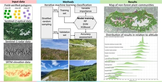
1. Introduction
Mountainous plant communities are made up of highly specialised plant species, resulting in distinct and biodiverse ecosystems [1]. These ecosystems provide a refuge for a wide range of wildlife [2] including many endemic plant species that have developed their specific habitats located in differentiated belts, which depend strictly on the elevation, aspects, and slopes. The documented results of climate change have highlighted dynamic alterations in mountain ecosystems. One of the most visible impacts is the increased rates of green-up [3], which is the phenomenon of vegetation greening earlier in the spring. Additionally, biotic change, which refers to changes in the distribution and abundance of plant species within an ecosystem, is also becoming more apparent in mountain summits [4]. These changes have far-reaching consequences for ecosystem stability, functioning, species richness, and biodiversity in different vegetation belts [5] and change soil and hydrological conditions [6]. Furthermore, this phenomenon is having a direct impact on pasture management [7]. Mountain ecosystems are sensitive to disturbance, so monitoring of plant communities is a focal indicator of ongoing alterations. For this reason, as well as the fact that various habitats are close to each other, e.g., tundra and valley ecosystems, high mountain areas are the best indicators of global changes. Changes occur more rapidly in non-forest communities, making continuous monitoring necessary, as traditional vegetation maps quickly become outdated. It is therefore necessary to develop solutions by using remote sensing methods to produce accurate maps of mountain vegetation.
Remote sensing technologies play an integral role in vegetation studies, enabling the monitoring of large swaths of land. However, depending on the research object and the character of the analyses, there is a trade-off between remote sensing platforms, sensors, and potential implementation. High performance is provided by aerial hyperspectral data for distinguishing detailed spectral and radiometric characteristics and also UAV data, which offer high spatial accuracy, have been successfully used [8]. However, due to the method of data acquisition, this makes it difficult to apply them on a large scale focusing on local case studies. Additionally, it is difficult to carry out repeatable surveys and continuous monitoring of vegetation, which is a key element in understanding the dynamics and character of the ongoing changes [9]. Therefore, satellite data are more effectively used in vegetation monitoring, providing large-area coverage and constant revisit time ensuring capture of ongoing changes. For high-resolution data, Hubert-Moy et al. [10] applied SPOT-7 data to mapping marsh communities, achieving F1-scores of 0.77–0.99, followed by WorldView-2, while Greaves et al. [11] based on airborne lidar, 20 cm RGBN imagery and Random Forest achieved 86% overall accuracy for tundra vegetation, and Meng et al. [12], using Gaofen-1 satellite for alpine grassland communities, obtained producer accuracy between 67 and 96%. However, with the reduced number of spectral bands of high-resolution satellites, it is limited to identify plant communities with unique spectral characteristics [13].
Therefore, the use of open satellite data from Landsat or Sentinel-2 satellites allows for more frequent revisits and more spectral bands with a decrease in spatial resolution. Rapinel et al. [14] concluded that Sentinel-2 data can be used effectively to map numerous plant communities of Natura 2000 sites to obtain F1-scores ranging from 0.31 to 0.99 depending on vegetation type. Additionally, using imagery compositions acquired from different dates, Le Dez et al. [15] managed to classify with the random forest algorithm 39 riparian habitats, achieving an overall accuracy of 76% for single date to 99% for multi-temporal dates. Likewise, Hubert-Moy et al. [16], using multi-temporal Sentinel-2 data to classify four heath habitats with similar spectral characteristics, obtained results with a wide range of user accuracy of 20–85%, UA of 50–79%, and producer, showing that the use of additional data is also necessary, especially for communities where the species mix. As vegetation is closely linked to habitat factors, it is useful to use environmental and bioclimatic variables [17]. One of the difficulties in applying this is the transferability of the solution due to the lack of harmonisation and consistency of data collected in different regions of the world. To achieve improved results in mountainous areas, where vegetation is closely linked through altitudinal zonation, Waśniewski et al. [18] demonstrated that the use of digital elevation model (DEM) data increased results by 22% in overall accuracy for mapping land cover classes over a complex mountain area. In coastal and mountainous areas, where there are few optical scenes acquired with satellites due to the abundance of cloud cover, radar data, which retrieve data independent of atmospheric conditions and time of day, provides complementary information on vegetation structure. Xiao et al. [19] demonstrated that Sentinel-1 open radar data combined with Sentinel-2 data successfully mapped mangrove forests with a high accuracy F1-score of 0.89–0.97. The most commonly used and best-performing machine learning classification algorithms are random forest and support vector machines [20], as well as XGBoost, being applied successfully to environmental parameter modelling with satellite data [21]. Despite using various methodologies over satellite data, there is a significant lack of detailed vegetation mapping at a phytosociological level [22].
To summarise the overview of the aforementioned research, there is a notable lack of detailed vegetation mapping compiled at a phytosociological level instead of basing it solely on common land cover classes, which prevents more complex studies such as habitat delineation for individual wildlife or complex botanical studies. However, mapping individual species is not effective information, while investigating characteristic combinations of plant co-occurrences, i.e., communities, more closely reflects the variety of the area and is a more effective indicator of change and biodiversity. Also, the potential of radar data in classifying non-forested mountain communities has not been well investigated, especially individual components such as orbits and polarisations. Thus, Sentinel-1 captures features such as structure and surface roughness and Sentinel-2 spectral features. The frequent cloud cover over mountain areas and the short growing season makes limited access to the number of high-quality optical satellite images, thus radar data can provide additional input.
Therefore, this study presents an approach for mapping non-forest vegetation with iterative machine learning techniques. Plant communities were classified in a high-value natural area with complex terrain using a fusion of Sentinel-2 optical and Sentinel-1 microwave data, and topographic variables. The testing of numerous classification scenarios as well as the importance of individual spectral bands determined the most relevant variables for the identification of mountain vegetation, and through the application of iterative methods, the accuracy ranges that the classes achieved were obtained. Based on the trained algorithms, the first coherent map of the non-forest vegetation of the Tatra Mountains was produced.
2. Materials and Methods
2.1. Study Area
The study area includes the Tatra Mountains, which are a UNESCO Transboundary Biosphere Reserve covering 95,000 ha of Polish and Slovak National Parks (Figure 1). The area is characterised by varied topography with elevations ranging from 700 to 2655 m a.s.l. and steep slopes. High topographic diversity and significant denivelations, which mean variable of water vapour content in the height profile, directly influence the amount of sun radiation reaching the plants, forcing a need for defence mechanisms, e.g., waxes covering the leaves, an increased share of protective chlorophyll pigments (e.g., carotenoids and xanthophylls), as well as smaller leaf surface, which are additionally exposed to drying, also by cold winds, hence the change in plant morphology and physiology with the altitude gradient. Mean annual air temperature varies from +4 °C in the lowest parts to −2 °C in the highest parts) and from the 1980s, it began to increase at a rate of 0.5 °C per decade [23]. Extreme weather with vast temperature variations, strong winds, long snow cover duration, and high UV radiation causes a series of adjustments of the vegetation, resulting in unique plant communities with high biodiversity (Figure 2). However, the vegetation is exposed to several risks including excessive tourism and anthropogenic factors [24], causing trampling, and decreasing the health of the plants [25]. Non-forest plant communities are also threatened by invasive species [26] and overgrowth of natural mountain meadows by forests and shrubs [27]. This results in a high need for continuous and repeated monitoring of mountain non-forest plant communities.
2.2. Satellite Data
For the analyses, three datasets were used: optical Sentinel-2 data, Sentinel-1 radar data, and Shuttle Radar Topographic Mission (SRTM) elevation data. The Sentinel-1 mission provides data from a dual-polarisation VV + VH (VV–vertical transmit and vertical receive; vertical transmit and horizontal receive) C-band synthetic aperture radar instrument. Sentinel-1 data were processed in the Google Earth Engine cloud environment [28]. Ground range detected (GRD) ready-to-use products of backscatter coefficient expressed in units of decibels (dB) with a pixel size of 10 m were obtained. The imagery was acquired for the Tatra area for 2019–2022 from May to November (7 months), which included four relative orbits. Due to the failure of the Sentinel-1B satellite [29], there has been a reduction in the number of available scenes in 2022 (Table 1). The monthly median composition was calculated [30]. Sentinel-1 data were split into ascending and descending orbits during processing because this is a mountainous area and the acquisition of a different local incidence angle has an impact on the discrepancy in backscatter coefficient values. Then, Sentinel-1 pixel grids were aligned with Sentinel-2 pixel grids.
Sentinel-2 level 2A optical data including 12 spectral bands were acquired for 2019–2022 for a total of 20 dates (Figure 3) with a cloud cover of less than 5% over the study area. The cloudless images acquired for the year were between four and six. The area included two tiles (34UDV, 34UCV) located in orbits 079 and 036. The data were processed by European Space Agency SNAP 8.0 software, where the bands were resampled to a uniform resolution of 10 m. Due to the character of the mountainous area, the prevailing cloud cover prevents the acquisition of high-quality images, most of which are available from November and September.
For the acquisition of elevation data, the 1 Arc-Second Global (~30 m pixel size) derived from the Shuttle Radar Topography Mission was utilised [31]. Topographic derivatives, including slope and aspect maps represented in degree values, were computed from the SRTM digital elevation model. The topographic feature data were resampled and aligned with the Sentinel-2 pixel grid. Topographic derivatives based on SRTM were integrated with both Sentinel-2 optical and Sentinel-1 radar imagery into one raster stack, which was used by selecting layers for specific classification scenarios.
2.3. Reference Dataset
The locations of plant communities were collected using a GNSS (global navigation satellite system) receiver during field campaigns carried out between 2021 and 2023, during which a total of 968 polygons were acquired during different parts of the growing season to more effectively distinguish communities through variable phenology and discolouration. Thirteen plant community classes and two background classes were distinguished (Table 2). The focus was on the level of detail of the association (Ass.) units, which were aggregated into larger alliance (All.) units due to the small areas and transitional nature of some communities.
2.4. Classification, Accuracy Assessment, and Variable Importance
For the classification, random forest [32], support vector machines [33], and XGBoost [34] algorithms were used due to the high performance achieved in machine learning applications in remote sensing [20]. To minimise the impact of variability of heterogeneous vegetation patches, the classification process was based on field-verified polygons, which allowed for the acquisition of randomised generated pixels representing training and verification pixel sets for classification in a 50:50 ratio using stratified random sampling method, so that pixels from one polygon could only be in one of the sets to maintain the independence condition [35]. This procedure was repeated 100 times, allowing us to determine the range of classification accuracies representing different habitats in each iteration. The classification results were presented in the form of box plots to capture a diversity of the outcomes, and the optimal training sets (the highest median F1-score) for the final classifications. The median F1-score values (Q2) were used to select the optimal sets of analysed image data (Sentinel-1, Sentinel-2, topographic derivatives), and the classifier for identifying plant communities. The statistical data allowed us to obtain the ranges of accuracies that the classes achieve giving a wider insight into the results (Figure 4).
The assessment of classification accuracy is mainly based on the overall accuracy (OA), while the F1-score is the harmonic mean of producer accuracy (PA) and user accuracy (UA), providing low-biased results. For calculating the variable importance of individual Sentinel-2 spectral bands to test their significance on the classification results, commonly used measures of mean decrease accuracy and mean decrease Gini were used. Before the classifications, tuning of the algorithm hyperparameters was performed using a grid search method that was used together with a 10-fold cross-validation for each scenario due to the different number of input variables (Table 3). In the case of random forest, a fixed value of ntree = 500 was used, and the parameter mtry was adjusted. In the case of SVM, the radial basis function (RBF) kernel was selected due to the best performance [36] and the cost and gamma parameters were tested.
The classification by scenario was then carried out by checking the effect of each variable on the accuracy of results. Based on the highest results of the mean F1-measure for all classes, a prediction of the resulting maps was carried out. The resulting rasters were then filtered with a 3 × 3 median filter for noise reduction, preparing the final vegetation maps of the Tatra Mountains.
3. Results
The result of the work is a map of dominant non-forest communities in the high-mountain area of the Tatra Transboundary Biosphere Reserve (UNESCO M&B), which, along with the Alps, Pyrenees, Scandinavian Mountains, and the Caucasus, is among the most valuable high-mountain areas in Europe with a developed alpine zone and high-mountain tundra. The obtained results confirmed the usefulness of available Sentinel satellite data and open-source machine learning algorithms, which will allow monitoring changes taking place in various parts of Europe with an accuracy oscillating around 90% (overall accuracy), but it is required to develop common legend units for vegetation maps.
3.1. Overall Results of Individual Classifiers and Acquisition Dates
In the first stage, the random forest, support vector machines, and XGBoost algorithms (Figure 5) were tested on datasets with the highest information potential. The best overall accuracy results were obtained by RF (82–97%) which was selected for detailed analyses, and SVM (88–94%), while poorer results were obtained by XGBoost (78–83%), so it was decided not to use it for further analyses and detailed scenarios because the achieved accuracy results were significantly lower (by 12% on average).
Analysing the individual scenarios for the random forest classifier based on the average F1-measure calculated for all classes (Figure 6), it can be observed that the best results are obtained by fusing optical and radar data with topographic data (0.88). Also, performing highly is the combination of optical data with topographic data (0.86), as well as with radar data itself (0.84). For Sentinel-2 data only, the accuracies are high (0.83), while for radar data, the results are much lower (0.59) even when combined with topographic variables (0.68). In terms of optical Sentinel-2 data acquisition, the best month on average was September (0.61), while the lowest results were obtained in November (0.50). Slight differences can be seen between the ascending and descending orbits of the radar data (by 0.02) as well as the VV and VH polarisations (by 0.01). By contrast, the lowest scores are achieved with Sentinel-1 data acquired for one year (0.40–0.48).
3.2. Results for Individual Vegetation Classes
Analysis of the mean F1-score values for each class (Table 4) resulted in values of 0.73–1.00 for random forest and 0.66–0.99 for support vector machines. Regarding Sentinel-2 optical data, this difference is better for SVM (0.69–0.99) relative to RF (0.51–0.99), but already, the addition of topographic variables changes the difference in favour of RF (0.74–0.99) to SVM (0.69–0.99). It can be seen that topographic variables increase the classification results by an average of 5%. The classes that increase the results the most are Adenostylion alliariae (+0.25), Arrhenatherion and Polygono-Trisetion (+0.09), Rubetum idaei (+0.08), and other non-forest (+0.07). For Sentinel-1 radar data, results are, however, obtained with a wide range for the algorithms: RF (0.19–0.95) as well as SVM (0.36–0.96). In the case of classes, Arrhenatherion and Polygono–Trisetion (0.76) and also other non-forest communities (0.88) are well classified. For the other classes, the radar data F1-score is low (average 0.67) and these performances cannot be considered satisfactory. Analysing the results obtained for the individual classes, it can be seen that the classes included in the broadly defined alpine grasslands average high scores of 0.84 for the best scenario. The highest values are achieved by Luzuletum alpino-pilosae (0.92), as well as Festuco versicoloris-Agrostietum alpinae (0.89), and those with slightly lower scores are Calamagrostion (0.87) and Nardion (0.86). For Festuco versicoloris-Seslerietum tatrae and Oreochloo distichae-Juncetum trifidi, the scores are lower, 0.78 and 0.73, respectively. Regarding the low shrubs type classes, the average for the best scenario is 0.83. The best-scoring class consists of Vaccinietum myrtilli (0.88) and also Rubetum idaei (0.86), followed by the slightly lower Empetro-Vaccinietum (0.81) and weaker Adenostylion alliariae (0.78). Other classes not included in the broader groups score high with other non-forest (0.91) and rocks and scree communities (0.97), except the class Arrhenatherion and Polygono-Trisetion, which scores lower (0.78). Background class scores are high (above 0.95), which shows that it does not mix with the target classes and has been well differentiated and masked. Although some classes in the analysis recognised that they scored lower, this should still be considered to be high in the overall context as it is above the 0.73 F1-score.
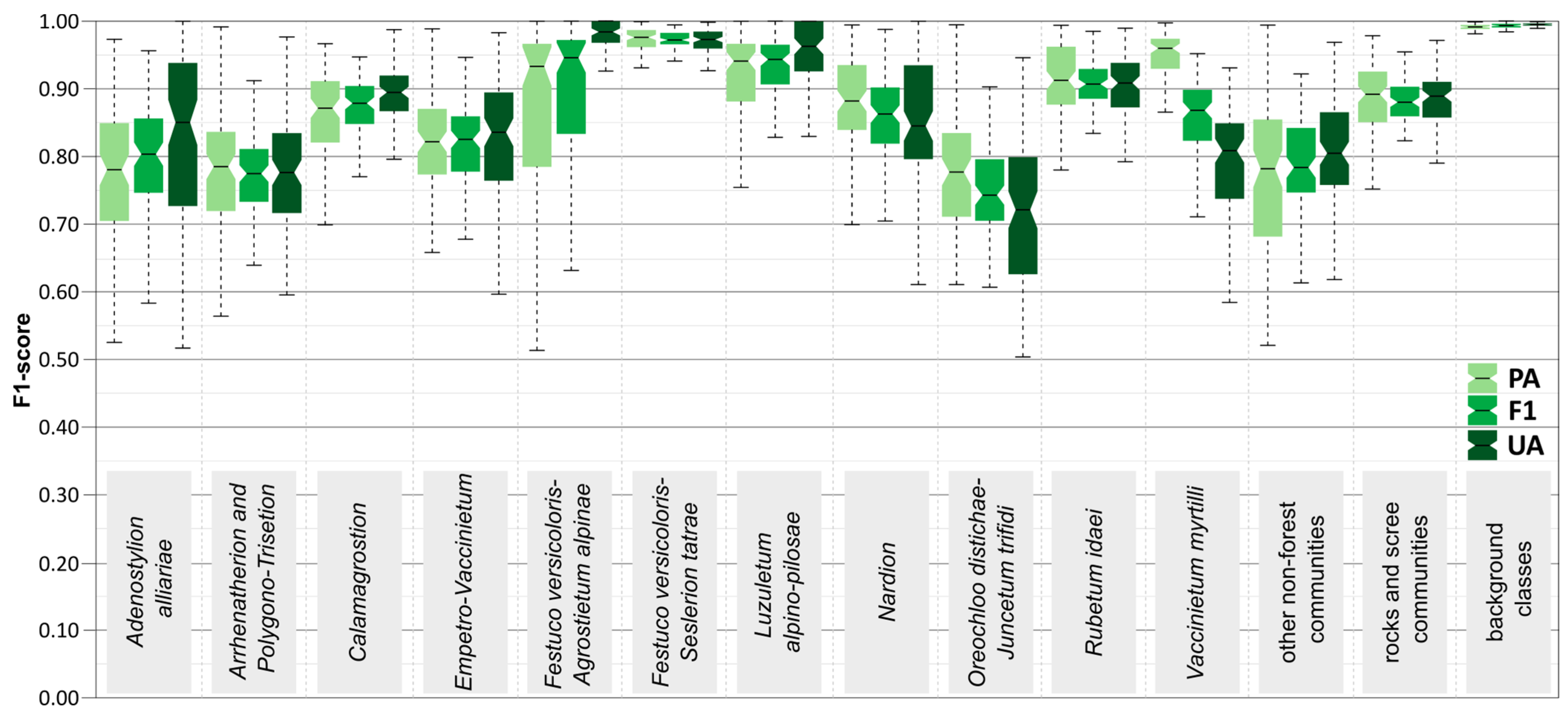
From an analysis of the distribution of random forest classifier scores (Figure 7), it can be observed that the median F1-score is above 0.73 for all classes, with ten classes scoring above 0.80 and five above 0.90. Some of the highest scores and at the same time with the narrowest interquartile range (IQR) are obtained for Festuco versicoloris–Seslerietum tatrae (0.98), as well as Luzuletum alpino-pilosae (0.93) and Rubetum idaei (0.96). Lower scores are obtained for the classes Oreochloo distichae–Juncetum trifidi (0.73) and Adenostylion alliariae (0.81), which are also characterised by a wide interquartile range. In the class examples analysed, the largest difference between UA and PA was achieved for the class Vaccinietum myrtilli, where the median producer accuracy for the class was 97% and the median user accuracy was 81%; this means that although 97% of the reference areas of this class were correctly identified, only 81% of the areas identified in the classification as Vaccinietum myrtilli were, in fact, this class. The opposite trend is for the class Adenostylion alliariae, where the median accuracy value of the producer is lower than the user accuracy by 8%, meaning that there were more areas of the class Adenostylion alliariae than were identified (Figure 6).
3.3. Relevance of Input Data
Based on the variable importance results (Figure 8), it can be seen that both in the case of mean decrease accuracy and mean decrease Gini, the most informative bands are B4, B3, and B2, which are associated with the 10 m Sentinel-2 bands. The spectral bands B4, B3, and B2 of the Sentinel-2 satellite imagery correspond to specific wavelengths within the visible and near-infrared spectrum. Band 2 is particularly valuable for discriminating soil and vegetation; this band is absorbed by chlorophyll, resulting in darker appearances of vegetation. In contrast, Band 3 predominantly reflects green light, making it essential for discerning different types of vegetation. Band 4, on the other hand, is highly reflective of dead foliage and aids in the identification of vegetation types. By emphasizing the significance of these bands, it becomes apparent that they contain crucial information necessary for the intended analysis or application. In the case of topographic variables, the digital elevation model and slope proved to be the most informative, while exposure is a less important factor.
3.4. Maps of Non-Forest Vegetation Occurrence
Based on random forest achieving the highest results, a first coherent map of non-forest vegetation was prepared for the Tatra area (Figure A1), as well as a comparison of classifiers (Figure 9) for selected 1.5 × 1.5 km areas of the Park in areas of high heterogeneity to test the effectiveness of the classification. In the case of SVM, there is a minor overestimation of the less frequent classes in favour of common classes. With RF, there is greater generalisation and a focus on large classes and overall characteristics.
4. Discussion
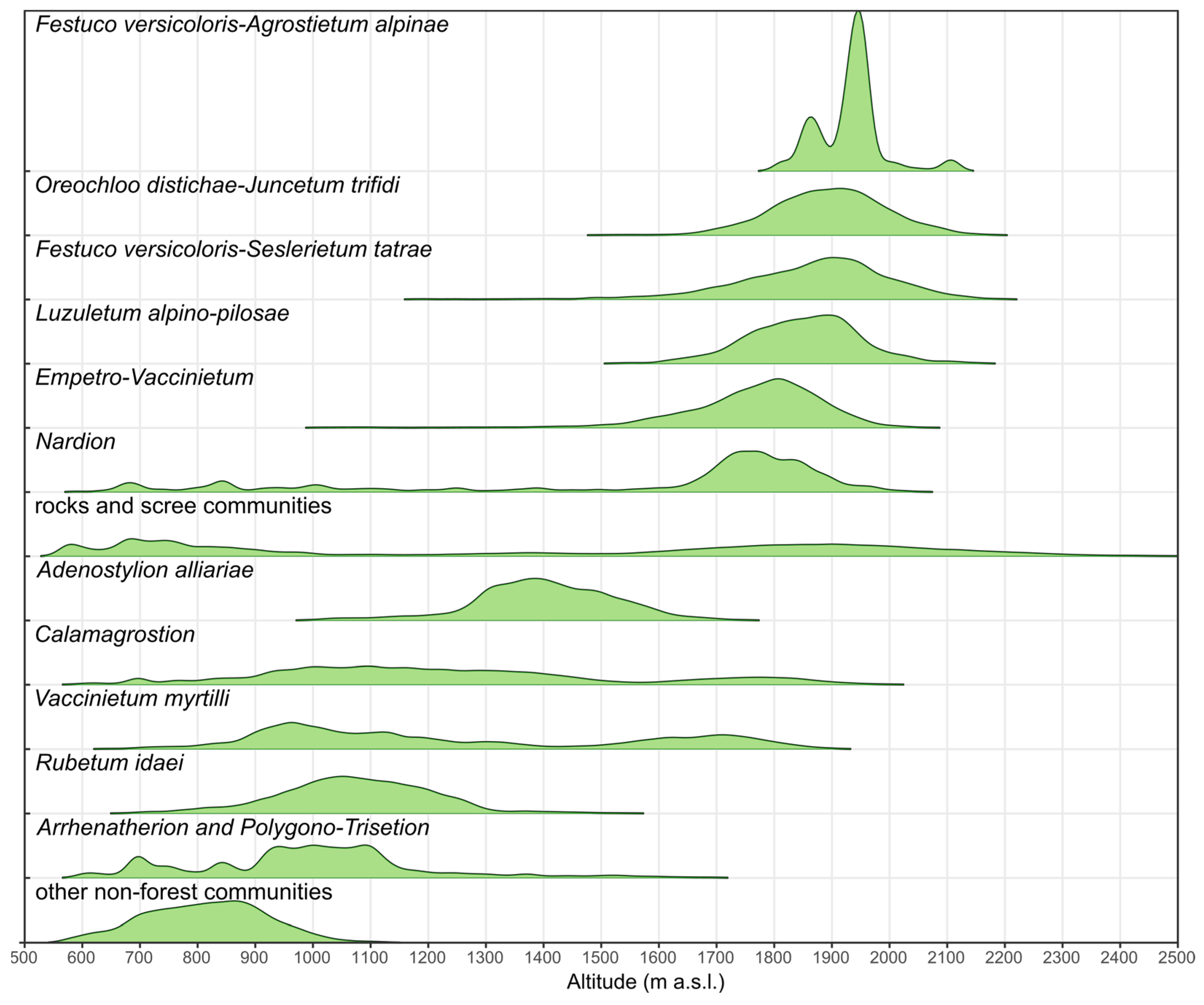
Achieved accuracy results are considered satisfactory (overall accuracy 93–97%), enabling the preparation of accurate vegetation maps for the entire Tatra area. Comparison of the location of individual classes based on the best-case scenario to the digital elevation model (Figure 10) shows the relationship of location to altitude. Consistent with the general occurrence, the class Vaccinetum myrtylii is lower and Emperto-Vaccinetum occupies higher positions. The lowest positions are occupied by other non-forest vegetation and low Rubetum idaei, which is mainly at the forest level, as well as hay meadows (Arrhenatherion and Polygono–Trisetion), alpine grassland classes that occupy some of the highest altitudes, covering areas of 1600–2200 m a.s.l. Due to the complex nature of the Tatra Mountains, the resolution of SRTM data may not be as accurate due to the steep slopes and sharp ridges present; therefore, results may vary. Also, patches of vegetation with a small area covered by shade may not have been detected especially those occurring in the highest parts of the mountains.
Analysing the results for individual years shows that despite a similar number of scenes (4–6), there is a large difference in the results obtained between years (by 0.10 F1-score), indicating that the date of acquisition is of great importance due to phenology and vegetation discolouration and the capture of spectral features. In the case of years where there is a little time gap, as in 2020 (F1-score: 0.68), scenes were only acquired between August and September, and also 2021 (F1-score: 0.70) the scenes from August to November were captured. For the wider range of acquired scenes in 2022 (F1-score: 0.78) from May to November and 2019 (F1-score: 0.74) from July to November, higher scores were obtained. Thereby, it reveals the importance of providing not only the number of images but also the time interval between images in which more spectral variation appears, enabling the capture of the characteristics of the plant communities considered. This was also proven by Macintyre et al. [37] for mapping the vegetation of low shrubs and trees on the multitemporal Sentinel-2, where a strong influence of phenology and the spectral response of the target classes for the autumn and spring seasons was observed. The Sentinel-2 multi-temporal optical data proved to be the most effective in classification (mean F1-score: 0.83), while the addition of topographic features in the area of varied terrain improved the results by 3%.
The radar data on impact by itself does not achieve high performance (mean F1-score: 0.59), but its addition to the optical data as a support allows for a 2% improvement in results. Radar data in the mountains are especially important, as acquisition from two ascending and descending orbits allows information to be captured from slopes that can often be covered by shadows on optical imagery. The beneficial impact of radar data was also confirmed by Dobrinić et al. [38] for land cover mapping, obtaining the highest results for the combination of S-1 with S-2 (OA: 92%), but lower for S2 (OA: 89%) and S1 (OA: 79%) alone. For Sentinel-1 data, the reduced number of radar scenes as a result of Sentinel-1B failure in 2022 did not affect classification accuracy. The year 2022 turned out to be a good year for classification where the number of scenes halved, achieving accuracies (mean F1-score: 0.43) comparable to other years (0.41–0.47) of S1, which shows that this number of images is sufficient.
In the classification undertaken with iterative machine learning methods, algorithms such as random forest and support vector machines performed well. Due to the spatial resolution of 10 m and the high heterogeneity of the classes, the input for classification was based solely on pixel values and not contextual neighbourhood information. For this reason, deep learning algorithms based on spatial relationship information between classes were not chosen. This was also confirmed by Heydari and Mountrakis [39], who used the support vector machine algorithm to obtain comparable results (OA: 65–98%) to deep learning methods (OA: 64–98%) on a diverse set of study sites. Investigating the impact of variable importance, it can be seen that the digital elevation model proves to be the most useful, which is also confirmed by Dobrinić et al. [38] in an analysis of mean decrease accuracy. Regarding Sentinel-2 spectral bands, blue (B2), red (B3), and green (B4) were found to be the most informative, which have the highest spatial resolution of 10 m in the Sentinel-2. It is related to the high discontinuity and patchwork of the occurring classes, thereby discriminating them for the bands with the highest resolution.
By considering the results for individual plant communities, it is important to take into account the region, the number of communities, their homogeneity, and the size of vegetation patches, as well as the co-occurrence of similar vegetation classes that can mix spectrally. Vegetation classification is most often subjected to Natura 2000 sites due to legal directives imposing reporting obligations, through which numerous methodologies have been developed to achieve high (>85% OA) accuracy results [40,41]. Wetland areas with abundant plant communities are also of great research interest [42]. Here, radar data are most often used due to the strong interaction of microwaves with water, allowing to obtain high accuracies of 90.0% ± 0.5% OA [43].
A limited number of studies focus on the mapping of specific plant communities in mountain areas. By comparing the results obtained to other mountain areas, the use of additional data and techniques is particularly important, as single Sentinel-2 imagery does not achieve high results and is not able to compete with hyperspectral data. Kupková et al. [44], for the mountain areas, obtained high scores (84%) for hyperspectral data but low scores (OA: 58%) for a single Sentinel-2 imagery from August based on the SVM classifier. Individual classes scored lower by a dozen to several dozen points of F1-score, such as Vaccinium vegetation (0.54; our result: 0.88), Alpine heathlands (0.40; our result: 0.81), Calamagrostis villosa stands (0.37; our result: 0.87), and Nardus stricta stands (0.50; our result: 0.86). Marcinkowska-Ochtyra et al. [45] confirmed the importance of APEX hyperspectral data and SVM classifier for 21 high-mountain non-forest classes (74.39% OA), while eight generalized vegetation types achieved 90.72% (APEX), and 78.25% (EnMAP simulated data). For the Himalayan area as well, multi-temporal Landsat 8 data resulted in an overall accuracy of 89% for mapping alpine grassland cover [46]. For mountainous areas, the use of topographic variables is valuable and has been shown to increase accuracy results by 3–5% OA. This was also confirmed by Mishra et al. [47] who mapped Sentinel-2 mountain vegetation using the random forest for the western Himalayan foothills using SRTM data with calculated topographic variables, achieving 70–87% overall accuracy.
Concerning the applied method of iterative classifications using machine learning algorithms, multi-sensor and multi-temporal remote sensing data as well as polygons acquired and verified in the field, it enables an effective statistical estimation of the results of the individual classes. A pilot study on a small fragment of Tatra Mountains [48] proved that the applied method shows a robust improvement, where an increase in accuracy of classes such as Calamagrostietum (0.86 now 0.87), Luzuletum alpino-pilosae (0.85 to 0.92 in this study), and Festuco versicoloris–Agrostietum alpinae (0.75 to 0.89 in this study). Only the class Oreochloo distichae–Juncetum trifidi is lower (0.83 to 0.73 in this study), but the number of distinguished plant communities has increased which has resulted in a stronger mixing of classes. The method used is transferable and also allows the mapping of other vegetation types with high accuracy, such as woody species. This is confirmed by Kluczek et al. [49], who classified 13 woody species (six broadleaves and seven coniferous) based on Sentinel-2’s dense multi-temporal dataset (more than 20 images) as well as SRTM elevation data. This has resulted in accuracies of more than 0.80 F1-score for each class. The method was also implemented in another study area (the Karkonosze mountain range) with satisfactory results (F1-score 0.67–0.91 for four tree species) [50]. It was also used to map the occurrence of individual invasive species such as goldenrod (Solidago spp.) with a high-performance F1-score of 0.85–0.95 [51]. Most relevant is the application of satellite imagery acquired at different dates, which enables the capture of individual unique spectral features of vegetation that vary spectrally over time through discrete phenological characteristics. This enables effective classification of different vegetation types in individual pixels of satellite images, even in areas of high heterogeneity, where it is not possible to distinguish the shapes of patches of vegetation types.
5. Conclusions
Mountain non-forest plant communities in an area with varied terrain and high-class heterogeneity can be mapped with high accuracy (0.87 mean F1-score; 97% overall accuracy) using a multi-temporal fusion of Sentinel-2 optical data with Sentinel-1 radar and topographic variables using iterative machine learning methods. Research has shown that topographic information has a high impact on classification accuracy, increasing individual class scores by up to 0.39 F1-score. For Sentinel-2 spectral bands, the most important are those with high resolution (10 m), that is red (B4), green (B3), and blue (B2).
The most important period for obtaining optical images with high scores is September, during which there is a very strong discolouration and pigmentation of the mountain vegetation, while the lowest scores are obtained in November when the vegetation is severely desiccated and no longer displays a high spectral variability. The random forest and support vector machines machine learning algorithms achieved high scores comparable to each other outperforming each other in individual scenarios.
For Sentinel-1 radar data, this does not achieve high accuracies, but it allows for maximising classification results. Nevertheless, radar data components such as individual polarisations or orbits are not relevant. The fusion of data acquired in one year for Sentinel-1 and Sentinel-2 together with topographic features is promising (0.84 in 2019; 0.83 in 2022), showing that data acquired in one year can be comparable to long time series, yielding results a few percent lower.
The iterative machine learning methods applied provided insight into the range of accuracy values achieved by each class, giving a more comprehensive insight and a better understanding of the performance characteristics of the classes; This indicates that in the case of wide interquartile distributions, it is essential to provide diverse training data that reflects the complexity of the distribution and facilitates effective mapping. In the future perspective, it is necessary to introduce monitoring based on the transferability of the trained algorithms to the following years as well as studies of occurring changes and processes, linking these to the specific environmental and bioclimatic variables.
Identifying and mapping vegetation in non-forest mountain areas can help in biodiversity conservation efforts. National park decision makers can use this information to monitor the distribution, fragmentation, and health of plant communities, and can implement conservation practices such as habitat restoration and invasive species control. Information on the distribution of different types of vegetation can help design tourist traffic so that it does not negatively affect valuable natural areas and strongly associated animal species, such as black grouse with non-forest habitats.
Author Contributions
Conceptualization, M.K. (Marcin Kluczek), B.Z. and M.K. (Marlena Kycko); methodology, M.K. (Marcin Kluczek) and B.Z.; software, M.K. (Marcin Kluczek); validation, M.K. (Marcin Kluczek), B.Z. and M.K. (Marlena Kycko); formal analysis, M.K. (Marcin Kluczek); investigation, M.K. (Marcin Kluczek); resources, M.K. (Marcin Kluczek), B.Z. and M.K. (Marlena Kycko); data curation, M.K. (Marcin Kluczek) and M.K. (Marlena Kycko); writing—original draft preparation, M.K. (Marcin Kluczek), B.Z. and M.K. (Marlena Kycko); writing—review and editing, M.K. (Marcin Kluczek), B.Z. and M.K. (Marlena Kycko); visualisation, M.K. (Marcin Kluczek); supervision, B.Z.; project administration, B.Z.; funding acquisition, B.Z. All authors have read and agreed to the published version of the manuscript.
Funding
The field campaign costs were covered by the Faculty of Geography and Regional Studies, University of Warsaw, grant no. SWIB 46/2022.
Data Availability Statement
Satellite data are publicly available online: Sentinel-1 and Sentinel- 2 images were acquired from the Copernicus Open Access Hub (https://scihub.copernicus.eu/; accessed on 1 August 2022) and SRTM elevation data from the EarthExplorer (https://earthexplorer.usgs.gov/; accessed on 1 August 2022). Reference polygons were acquired during field mapping by all authors, and the digital version was prepared by Marcin Kluczek.
Acknowledgments
The authors are grateful to the Tatra National Park for providing data and permitting us to conduct field research in the park.
Conflicts of Interest
The authors declare no conflicts of interest.
Appendix A
Figure A1.
Map of occurrence of non-forest communities in Tatra Mountains. Classification based on multi-temporal Sentinel-2 and Sentinel-1 data combined with topographic derivatives (digital elevation model, and slope and aspect maps) and random forest classifier.
Figure A1.
Map of occurrence of non-forest communities in Tatra Mountains. Classification based on multi-temporal Sentinel-2 and Sentinel-1 data combined with topographic derivatives (digital elevation model, and slope and aspect maps) and random forest classifier.

References
- Schuchardt, M.A.; Berauer, B.J.; Duc, A.L.; Ingrisch, J.; Niu, Y.; Bahn, M.; Jentsch, A. Increases in functional diversity of mountain plant communities is mainly driven by species turnover under climate change. Oikos 2023, 2023, e09922. [Google Scholar] [CrossRef]
- Inouye, D.W. Effects of climate change on alpine plants and their pollinators. Ann. N. Y. Acad. Sci. 2020, 1469, 26–37. [Google Scholar] [CrossRef] [PubMed]
- Choler, P.; Bayle, A.; Carlson, B.Z.; Randin, C.; Filippa, G.; Cremonese, E. The tempo of greening in the European Alps: Spatial variations on a common theme. Glob. Change Biol. 2021, 27, 5614–5628. [Google Scholar] [CrossRef] [PubMed]
- Steinbauer, M.; Grytnes, J.-A.; Jurasinski, G.; Kulonen, A.; Lenoir, J.; Pauli, H.; Rixen, C.; Winkler, M.; Bardy-Durchhalter, M.; Barni, E.; et al. Accelerated increase in plant species richness on mountain summits is linked to warming. Nature 2018, 556, 231–234. [Google Scholar] [CrossRef] [PubMed]
- Peringer, A.; Frank, V.; Snell, R.S. Climate change simulations in Alpine summer pastures suggest a disruption of current vegetation zonation. Glob. Ecol. Conserv. 2022, 37, e02140. [Google Scholar] [CrossRef]
- Kabir, R.; Pomeroy, J.; Whitfield, P. Are the effects of vegetation and soil changes as important as climate change impacts on hydrological processes? Hydrol. Earth Syst. Sci. 2019, 23, 4933–4954. [Google Scholar] [CrossRef]
- Zheng, L.; Li, D.; Xu, J.; Xia, Z.; Hao, H.; Chen, Z. A twenty-years remote sensing study reveals changes to alpine pastures under asymmetric climate warming. ISPRS J. Photogramm. Remote Sens. 2022, 190, 69–78. [Google Scholar] [CrossRef]
- Laporte-Fauret, Q.; Castelle, B.; Michalet, R.; Marieu, V.; Bujan, S.; Rosebery, D. Morphological and ecological responses of a managed coastal sand dune to experimental notches. Sci. Total Environ. 2021, 782, 146813. [Google Scholar] [CrossRef] [PubMed]
- Fassnacht, F.E.; Müllerová, J.; Conti, L.; Malavasi, M.; Schmidtlein, S. About the link between biodiversity and spectral variation. Appl. Veg. Sci. 2022, 25, e12643. [Google Scholar] [CrossRef]
- Hubert-Moy, L.; Fabre, E.; Rapinel, S. Contribution of SPOT-7 multi-temporal imagery for mapping wetland vegetation. Eur. J. Remote Sens. 2020, 53, 201–210. [Google Scholar] [CrossRef]
- Greaves, H.E.; Eitel, J.U.H.; Vierling, L.A.; Boelman, N.T.; Griffin, K.L.; Magney, T.S.; Prager, C.M. 20 cm resolution mapping of tundra vegetation communities provides an ecological baseline for important research areas in a changing Arctic environment. Environ. Res. Commun. 2019, 1, 105004. [Google Scholar] [CrossRef]
- Meng, B.; Yang, Z.; Yu, H.; Qin, Y.; Sun, Y.; Zhang, J.; Chen, J.; Wang, Z.; Zhang, W.; Li, M.; et al. Mapping of Kobresia pygmaea Community Based on Umanned Aerial Vehicle Technology and Gaofen Remote Sensing Data in Alpine Meadow Grassland: A Case Study in Eastern of Qinghai–Tibetan Plateau. Remote Sens. 2021, 13, 2483. [Google Scholar] [CrossRef]
- Sun, C.; Li, J.; Liu, Y.; Liu, Y.; Liu, R. Plant species classification in salt marshes using phenological parameters derived from Sentinel-2 pixel-differential time-series. Remote Sens. Environ. 2021, 256, 112320. [Google Scholar] [CrossRef]
- Rapinel, S.; Rozo, C.; Delbosc, P.; Bioret, F.; Bouzillé, J.-B.; Hubert-Moy, L. Contribution of free satellite time-series images to mapping plant communities in the Mediterranean Natura 2000 site: The example of Biguglia Pond in Corse (France). Mediterr. Bot. 2020, 41, 181–191. [Google Scholar] [CrossRef]
- Le Dez, M.; Robin, M.; Launeau, P. Contribution of Sentinel-2 satellite images for habitat mapping of the Natura 2000 site ‘Estuaire de la Loire’ (France). Remote Sens. Appl. Soc. Environ. 2021, 24, 100637. [Google Scholar] [CrossRef]
- Hubert-Moy, L.; Rozo, C.; Perrin, G.; Bioret, F.; Rapinel, S. Large-scale and fine-grained mapping of heathland habitats using open-source remote sensing data. Remote Sens. Ecol. Conserv. 2022, 8, 448–463. [Google Scholar] [CrossRef]
- Zeferino, L.B.; Souza, L.F.T.; Amaral, C.H.; Filho, E.I.F.; Oliveira, T.S. Does environmental data increase the accuracy of land use and land cover classification? Int. J. Appl. Earth Obs. Geoinf. 2020, 91, 102128. [Google Scholar] [CrossRef]
- Waśniewski, A.; Hościło, A.; Aune-Lundberg, L. The impact of selection of reference samples and DEM on the accuracy of land cover classification based on Sentinel-2 data. Remote Sens. Appl. Soc. Environ. 2023, 32, 101035. [Google Scholar] [CrossRef]
- Xiao, H.; Su, F.; Fu, D.; Lyne, V.; Liu, G.; Pan, T.; Teng, J. Optimal and robust vegetation mapping in complex environments using multiple satellite imagery: Application to mangroves in Southeast Asia. Int. J. Appl. Earth Obs. Geoinf. 2021, 99, 102320. [Google Scholar] [CrossRef]
- Subedi, M.R.; Portillo-Quintero, C.; Kahl, S.S.; McIntyre, N.E.; Cox Robert, R.D.; Perry, G. Leveraging NAIP Imagery for Accurate Large-Area Land Use/land Cover Mapping: A Case Study in Central Texas. Photogramm. Eng. Remote Sens. 2023, 89, 547–560. [Google Scholar] [CrossRef]
- Wieland, R.; Kuhls, K.; Lentz, H.K.H.; Conraths, F.; Kampen, H.; Werner, D. Combined climate and regional mosquito habitat model based on machine learning. Ecol. Modell. 2021, 452, 109594. [Google Scholar] [CrossRef]
- Kattenborn, T.; Eichel, J.; Fassnacht, F.E. Convolutional Neural Networks enable efficient, accurate and fine-grained segmentation of plant species and communities from high-resolution UAV imagery. Sci. Rep. 2019, 9, 17656. [Google Scholar] [CrossRef] [PubMed]
- Łupikasza, E.; Szypuła, B. Vertical climatic belts in the Tatra Mountains in the light of current climate change. Theor. Appl. Climatol. 2019, 136, 249–264. [Google Scholar] [CrossRef]
- Adach, S.; Wojtkowska, M.; Religa, P. Consequences of the accessibility of the mountain national parks in Poland. Environ. Sci. Pollut. Res. 2023, 30, 27483–27500. [Google Scholar] [CrossRef]
- Kycko, M.; Zagajewski, B.; Zwijacz-Kozica, M.; Cierniewski, J.; Romanowska, E.; Orłowska, K.; Ochtyra, A.; Jarocińska, A. Assessment of Hyperspectral Remote Sensing for Analyzing the Impact of Human Trampling on Alpine Swards. Mt. Res. Dev. 2017, 37, 66–74. [Google Scholar] [CrossRef]
- Kiełtyk, P.; Delimat, A. Impact of the alien plant Impatiens glandulifera on species diversity of invaded vegetation in the northern foothills of the Tatra Mountains, Central Europe. Plant. Ecol. 2019, 220, 1–12. [Google Scholar] [CrossRef]
- Palaj, A.; Kollár, J.; Michalová, M. Changes in the Nardus grasslands in the (Sub)Alpine Zone of Western Carpathians over the last decades. Biologia 2023, 79, 1081–1090. [Google Scholar] [CrossRef]
- Gorelick, N.; Hancher, M.; Dixon, M.; Ilyushchenko, S.; Thau, D.; Moore, R. Google Earth Engine: Planetary-scale geospatial analysis for everyone. Remote Sens. Environ. 2017, 202, 18–27. [Google Scholar] [CrossRef]
- Potin, P.; Colin, O.; Pinheiro, M.; Rosich, B.; O’Connell, A.; Ormston, T.; Gratadour, J.-B.; Torres, R. Status and Evolution of the Sentinel-1 Mission. In Proceedings of the IEEE International Geoscience and Remote Sensing Symposium, Kuala Lumpur, Malaysia, 17–22 July 2022; Volume 2022, pp. 4707–4710. [Google Scholar] [CrossRef]
- Luo, C.; Liu, H.; Lu, L.; Liu, Z.; Kong, F.; Zhang, X. Monthly composites from Sentinel-1 and Sentinel-2 images for regional major crop mapping with Google Earth Engine. J. Integr. Agric. 2021, 20, 1944–1957. [Google Scholar] [CrossRef]
- Farr, T.G.; Rosen, P.A.; Caro, E.; Crippen, R.; Duren, R.; Hensley, S.; Kobrick, M.; Paller, M.; Rodriguez, E.; Roth, L.; et al. The Shuttle Radar Topography Mission. Rev. Geophys. 2007, 45, RG2004. [Google Scholar] [CrossRef]
- Breiman, L. Random Forests. Mach. Learn. 2001, 45, 5–32. [Google Scholar] [CrossRef]
- Vapnik, V.N. The Nature of Statistical Learning Theory; Springer: New York, NY, USA, 1995; Volume 314. [Google Scholar] [CrossRef]
- Chen, T.; Guestrin, C. XGBoost: A Scalable Tree Boosting System. In Proceedings of the 22nd ACM SIGKDD International Conference on Knowledge Discovery and Data Mining, San Francisco, CA, USA, 13–17 August 2016; Association for Computing Machinery: New York, NY, USA, 2016; pp. 785–794. [Google Scholar] [CrossRef]
- Stehman, S.V.; Foody, G.M. Key issues in rigorous accuracy assessment of land cover products. Remote Sens. Environ. 2019, 231, 111199. [Google Scholar] [CrossRef]
- Tharwat, A. Parameter investigation of support vector machine classifier with kernel functions. Knowl. Inf. Syst. 2019, 61, 1269–1302. [Google Scholar] [CrossRef]
- Macintyre, P.; Niekerk, A.; Mucina, L. Efficacy of multi-season Sentinel-2 imagery for compositional vegetation classification. Int. J. Appl. Earth Obs. Geoinf. 2020, 85, 101980. [Google Scholar] [CrossRef]
- Dobrinić, D.; Gašparović, M.; Medak, D. Sentinel-1 and 2 Time-Series for Vegetation Mapping Using Random Forest Classification: A Case Study of Northern Croatia. Remote Sens. 2021, 13, 2321. [Google Scholar] [CrossRef]
- Heydari, S.; Mountrakis, G. Effect of classifier selection, reference sample size, reference class distribution and scene heterogeneity in per-pixel classification accuracy using 26 Landsat sites. Remote Sens. Environ. 2018, 204, 648–658. [Google Scholar] [CrossRef]
- Raab, C.; Stroh, H.G.; Tonn, B.; Meißner, M.; Rohwer, N.; Balkenhol, N.; Isselstein, J. Mapping semi-natural grassland communities using multi-temporal RapidEye remote sensing data. Int. J. Remote Sens. 2018, 39, 5638–5659. [Google Scholar] [CrossRef]
- Jarocińska, A.; Kopeć, D.; Niedzielko, J.; Wylazłowska, J.; Halladin-Dąbrowska, A.; Charyton, J.; Piernik, A.; Kamiński, D. The utility of airborne hyperspectral and satellite multispectral images in identifying Natura 2000 non-forest habitats for conservation purposes. Sci. Rep. 2023, 13, 4549. [Google Scholar] [CrossRef] [PubMed]
- Bhatnagar, S.; Gill, L.; Regan, S.; Naughton, O.; Johnston, P.; Waldren, S.; Ghosh, B. Mapping Vegetation Communities Inside Wetlands Using Sentinel-2 Imagery in Ireland. Int. J. Appl. Earth Obs. Geoinf. 2020, 88, 102083. [Google Scholar] [CrossRef]
- Peng, K.; Jiang, W.; Hou, P.; Wu, Z.; Ling, Z.; Wang, X.; Niu, Z.; Mao, D. Continental-scale wetland mapping: A novel algorithm for detailed wetland types classification based on time series Sentinel-1/2 images. Ecol. Indic. 2023, 148, 110113. [Google Scholar] [CrossRef]
- Kupková, L.; Cervená, L.; Suchá, R.; Jakešová, L.; Zagajewski, B.; Brezina, S.; Albrechtová, J. Classification of tundra vegetation in the Krkonoše Mts. National park using APEX, AISA dual and Sentinel-2A data. Eur. J. Remote Sens. 2017, 50, 29–46. [Google Scholar] [CrossRef]
- Marcinkowska-Ochtyra, A.; Zagajewski, B.; Ochtyra, A.; Jarocińska, A.; Wojtuń, B.; Rogass, C.; Mielke, C.; Lavender, S. Subalpine and Alpine Vegetation Classification based on Hyperspectral APEX and Simulated EnMAP images. Int. J. Remote Sens. 2017, 38, 1839–1864. [Google Scholar] [CrossRef]
- Pandey, A.; Singh, G.; Palni, S.; Chandra, N.; Rawa, J.; Singh, A.P. Application of remote sensing in alpine grasslands cover mapping of western Himalaya, Uttarakhand, India. Environ. Monit. Assess. 2021, 193, 166. [Google Scholar] [CrossRef] [PubMed]
- Mishra, A.P.; Rai, I.D.; Pangtey, D.; Padalia, H. Vegetation Characterization at Community Level Using Sentinel-2 SatelliteData and Random Forest Classifier in Western Himalayan Foothills, Uttarakhand. J. Indian Soc. Remote Sens. 2021, 49, 759–771. [Google Scholar] [CrossRef]
- Kluczek, M.; Zagajewski, B.; Kycko, M. Airborne HySpex Hyperspectral Versus Multitemporal Sentinel-2 Images for Mountain Plant Communities Mapping. Remote Sens. 2022, 14, 1209. [Google Scholar] [CrossRef]
- Kluczek, M.; Zagajewski, B.; Zwijacz-Kozica, T. Mountain Tree Species Mapping Using Sentinel-2, PlanetScope, and Airborne HySpex Hyperspectral Imagery. Remote Sens. 2023, 15, 844. [Google Scholar] [CrossRef]
- Zagajewski, B.; Kluczek, M.; Raczko, E.; Njegovec, A.; Dabija, A.; Kycko, M. Comparison of Random Forest, Support Vector Machines, and Neural Networks for Post-Disaster Forest Species Mapping of the Krkonoše/Karkonosze Transboundary Biosphere Reserve. Remote Sens. 2021, 13, 2581. [Google Scholar] [CrossRef]
- Zagajewski, B.; Kluczek, M.; Zdunek, K.B.; Holland, D. Sentinel-2 versus PlanetScope Images for Goldenrod Invasive Plant Species Mapping. Remote Sens. 2024, 16, 636. [Google Scholar] [CrossRef]
Figure 1.
Location of the study area the core and buffer zone of Tatra Transboundary Biosphere Reserve (red box on the left image; satellite image for Poland area: Sentinel-2 RGB median composition for June–August 2023; generated using Google Earth Engine; satellite image for the Tatras area: Sentinel-2 RGB 2020-08-22).

Figure 2.
Species adaptations of physiological and morphological processes allow the identification of spectral features recorded in multitemporal and multispectral satellite data of individual plant communities (view from the Kasprowy Wierch (location: 49°13′57″N, 19°58′53″E) towards the Western Tatras, photo credit: Bogdan Zagajewski).

Figure 3.
Sentinel-2 acquisition dates with the distribution of mean cloud cover based on the metadata of all available satellite scenes.
Figure 3.
Sentinel-2 acquisition dates with the distribution of mean cloud cover based on the metadata of all available satellite scenes.

Figure 4.
Iterative classification method scheme.

Figure 5.
Overall accuracy results of different scenarios (Explanation: S1–Sentinel-1, S2–Sentinel-2, TF–topographic features including digital elevation model, slope and aspect maps).
Figure 5.
Overall accuracy results of different scenarios (Explanation: S1–Sentinel-1, S2–Sentinel-2, TF–topographic features including digital elevation model, slope and aspect maps).

Figure 6.
Mean F1-score for classes based on acquisition date based on 100 iterations (explanation: S1—Sentinel-1, S2—Sentinel-2, TF—topographic features including digital elevation model, slope and aspect maps, ASC—ascending orbit, DSC—descending orbit).
Figure 6.
Mean F1-score for classes based on acquisition date based on 100 iterations (explanation: S1—Sentinel-1, S2—Sentinel-2, TF—topographic features including digital elevation model, slope and aspect maps, ASC—ascending orbit, DSC—descending orbit).

Figure 7.
Variation of the F1-score, producer accuracy (PA), and user accuracy (UA) values for classes based on 100 iterations using random forest algorithm and combined Sentinel-1 with Sentinel-2 and topographic features. For each box plot, the lower quartile (Q1) is the lower edge of the box, the median is the bar in the box, and the upper quartile (Q3) is the upper edge of the box.

Figure 8.
Variable importance on Sentinel-2 bands (mean decrease accuracy: digital elevation model = 18.0, slope = 9.7, aspect = 3.6; mean decrease Gini: digital elevation model = 9.7, slope = 2.9, aspect = 0.8).
Figure 8.
Variable importance on Sentinel-2 bands (mean decrease accuracy: digital elevation model = 18.0, slope = 9.7, aspect = 3.6; mean decrease Gini: digital elevation model = 9.7, slope = 2.9, aspect = 0.8).

Figure 9.
Comparison of obtained classification maps based on random forest and support vector machines with high-resolution orthophoto map (geographic coordinates represent centroids of polygons).
Figure 9.
Comparison of obtained classification maps based on random forest and support vector machines with high-resolution orthophoto map (geographic coordinates represent centroids of polygons).

Figure 10.
Ridgeline plots of mountain vegetation communities classification results (frequency) in relation to altitude based on the digital elevation model.
Figure 10.
Ridgeline plots of mountain vegetation communities classification results (frequency) in relation to altitude based on the digital elevation model.


Table 1.
Number of Sentinel-1 acquisitions per year.
| S1A | S1B | |||||
|---|---|---|---|---|---|---|
| ASC | DSC | ASC | DSC | Total | Mean Scenes per Month | |
| 2019 | 35 | 34 | 54 | 34 | 157 | 22 |
| 2020 | 36 | 35 | 52 | 35 | 158 | 23 |
| 2021 | 35 | 34 | 54 | 35 | 158 | 23 |
| 2022 | 35 | 33 | 0 | 0 | 68 | 10 |
Table 2.
Definitions of the considered classes for mountain vegetation mapping.
| Class | Description | No. of Sentinel-2 Pixels | No. of Polygons |
|---|---|---|---|
| Adenostylion alliariae | Low shrubs, mountain herbs | 405 | 22 |
| Arrhenatherion and Polygono-Trisetion | Mountain hay meadows | 1898 | 63 |
| Calamagrostion | Alpine grasslands | 1965 | 39 |
| Empetro-Vaccinietum | Low shrubs, heath communities | 527 | 27 |
| Festuco versicoloris-Agrostietum alpinae | Alpine calcareous grasslands | 163 | 12 |
| Festuco versicoloris-Seslerietum tatrae | Alpine calcareous grasslands | 730 | 29 |
| Luzuletum alpino-pilosae | Alpine grasslands | 102 | 18 |
| Nardion | Alpine grasslands | 355 | 28 |
| Oreochloo distichae-Juncetum trifidi | Siliceous alpine grasslands | 412 | 42 |
| Rubetum idaei | Shrubs with domination of raspberry | 920 | 56 |
| Vaccinietum myrtilli | Low shrubs with domination of Vaccinium myrtillus | 1394 | 50 |
| Other non-forest | Initial and degraded plant communities | 3215 | 63 |
| Rocks and scree communities | Vegetation and lichens growing on a loose bedrock or bare rock | 4116 | 75 |
| Forest (background) | Coniferous and deciduous forests plant communities | 21,674 | 430 |
| Water (background) | Stream and mountain lake waters | 9519 | 14 |
| Total | 47,395 | 968 |
Table 3.
Variables for classification scenarios with hyperparameters for random forest (RF) and support vector machines (SVMs).
Table 3.
Variables for classification scenarios with hyperparameters for random forest (RF) and support vector machines (SVMs).
| One Year | 2019–2022 | |||||||
|---|---|---|---|---|---|---|---|---|
| Dataset | No. of Variables | RF mtry | SVM Cost | SVM Gamma | No. of Variables | RF mtry | SVM Cost | SVM Gamma |
| S1 | 28 | 5 | 1 | 0.10 | 112 | 15 | 10 | 0.01 |
| S1 + TF | 31 | 5 | 1 | 0.10 | 115 | 15 | 10 | 0.01 |
| S2 | 48–72 | 7 | 1 | 0.10 | 240 | 25 | 100 | 0.01 |
| S2 + TF | 51–75 | 7 | 1 | 0.10 | 243 | 25 | 100 | 0.01 |
| S1 + S2 | 76–100 | 10 | 100 | 0.01 | 352 | 40 | 100 | 0.01 |
| S1 + S2 + TF | 79–103 | 10 | 100 | 0.01 | 355 | 40 | 100 | 0.01 |
Table 4.
Mean F1-score of classes for different scenarios.
| Class | S1 + S2 + TF | S1+ S2 | S2 + TF | S2 | S1 + TF | S1 | ||||||
|---|---|---|---|---|---|---|---|---|---|---|---|---|
| RF | SVM | RF | SVM | RF | SVM | RF | SVM | RF | SVM | RF | SVM | |
| Adenostylion alliariae | 0.78 | 0.70 | 0.59 | 0.68 | 0.76 | 0.82 | 0.51 | 0.77 | 0.41 | 0.41 | 0.25 | 0.36 |
| Arrhenatherion and Polygono–Trisetion | 0.77 | 0.75 | 0.70 | 0.74 | 0.79 | 0.77 | 0.71 | 0.76 | 0.71 | 0.76 | 0.63 | 0.71 |
| Calamagrostion | 0.87 | 0.82 | 0.87 | 0.82 | 0.87 | 0.88 | 0.86 | 0.88 | 0.51 | 0.67 | 0.49 | 0.65 |
| Empetro–Vaccinietum | 0.81 | 0.70 | 0.80 | 0.70 | 0.80 | 0.80 | 0.79 | 0.79 | 0.52 | 0.52 | 0.47 | 0.50 |
| Festuco versicoloris–Agrostietum alpinae | 0.89 | 0.95 | 0.89 | 0.95 | 0.88 | 0.96 | 0.88 | 0.96 | 0.88 | 0.86 | 0.74 | 0.82 |
| Festuco versicoloris–Seslerietum tatrae | 0.78 | 0.66 | 0.77 | 0.65 | 0.78 | 0.75 | 0.76 | 0.75 | 0.58 | 0.60 | 0.46 | 0.56 |
| Luzuletum alpino-pilosae | 0.92 | 0.77 | 0.92 | 0.76 | 0.88 | 0.80 | 0.88 | 0.80 | 0.58 | 0.60 | 0.19 | 0.51 |
| Nardion | 0.86 | 0.86 | 0.85 | 0.86 | 0.84 | 0.89 | 0.84 | 0.89 | 0.70 | 0.72 | 0.64 | 0.69 |
| Oreochloo distichae–Juncetum trifidi | 0.73 | 0.67 | 0.72 | 0.68 | 0.74 | 0.69 | 0.73 | 0.69 | 0.64 | 0.54 | 0.53 | 0.54 |
| Rubetum idaei | 0.86 | 0.86 | 0.79 | 0.85 | 0.86 | 0.91 | 0.77 | 0.90 | 0.55 | 0.70 | 0.50 | 0.66 |
| Vaccinietum myrtilli | 0.88 | 0.84 | 0.87 | 0.84 | 0.87 | 0.86 | 0.85 | 0.86 | 0.61 | 0.72 | 0.57 | 0.66 |
| Other non-forest | 0.91 | 0.89 | 0.88 | 0.88 | 0.91 | 0.89 | 0.87 | 0.88 | 0.84 | 0.88 | 0.77 | 0.83 |
| Rocks and scree communities | 0.97 | 0.82 | 0.97 | 0.82 | 0.97 | 0.92 | 0.96 | 0.92 | 0.83 | 0.83 | 0.74 | 0.79 |
| Forest (background) | 0.99 | 0.99 | 0.99 | 0.99 | 0.99 | 0.99 | 0.99 | 0.99 | 0.94 | 0.96 | 0.93 | 0.96 |
| Water (background) | 1.00 | 0.95 | 1.00 | 0.95 | 0.99 | 0.99 | 0.99 | 0.99 | 0.97 | 0.96 | 0.95 | 0.95 |
Disclaimer/Publisher’s Note: The statements, opinions and data contained in all publications are solely those of the individual author(s) and contributor(s) and not of MDPI and/or the editor(s). MDPI and/or the editor(s) disclaim responsibility for any injury to people or property resulting from any ideas, methods, instructions or products referred to in the content. |
© 2024 by the authors. Licensee MDPI, Basel, Switzerland. This article is an open access article distributed under the terms and conditions of the Creative Commons Attribution (CC BY) license (https://creativecommons.org/licenses/by/4.0/).
Share and Cite
MDPI and ACS Style
Kluczek, M.; Zagajewski, B.; Kycko, M. Combining Multitemporal Optical and Radar Satellite Data for Mapping the Tatra Mountains Non-Forest Plant Communities. Remote Sens. 2024, 16, 1451. https://doi.org/10.3390/rs16081451
AMA Style
Kluczek M, Zagajewski B, Kycko M. Combining Multitemporal Optical and Radar Satellite Data for Mapping the Tatra Mountains Non-Forest Plant Communities. Remote Sensing. 2024; 16(8):1451. https://doi.org/10.3390/rs16081451
Chicago/Turabian StyleKluczek, Marcin, Bogdan Zagajewski, and Marlena Kycko. 2024. "Combining Multitemporal Optical and Radar Satellite Data for Mapping the Tatra Mountains Non-Forest Plant Communities" Remote Sensing 16, no. 8: 1451. https://doi.org/10.3390/rs16081451
Note that from the first issue of 2016, this journal uses article numbers instead of page numbers. See further details here.