Wind Profile Reconstruction Based on Convolutional Neural Network for Incoherent Doppler Wind LiDAR

 , , and
Abstract
:
1. Introduction
2. Methods
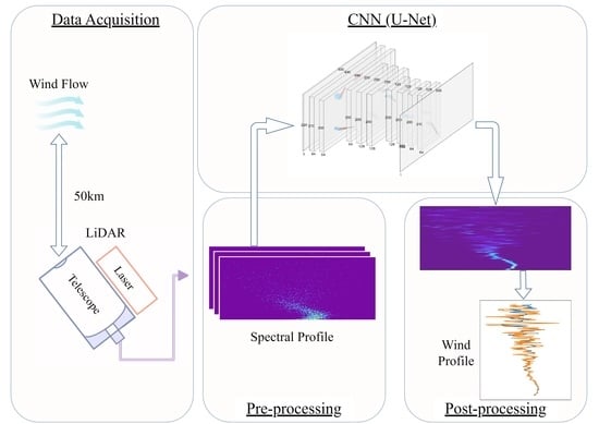
2.1. Data Acquisition
2.1.1. Measurement from ICDL
2.1.2. ECMWF: ERA5 Dataset
2.2. Simulation of Wind Profile Reconstruction
2.2.1. Error Calculation
2.2.2. Wind Perturbation
2.2.3. Wind Profile Reconstruction
2.3. Machine Learning
2.3.1. CNN Structure
2.3.2. Pre-Processing
2.3.3. Post-Processing
3. Results
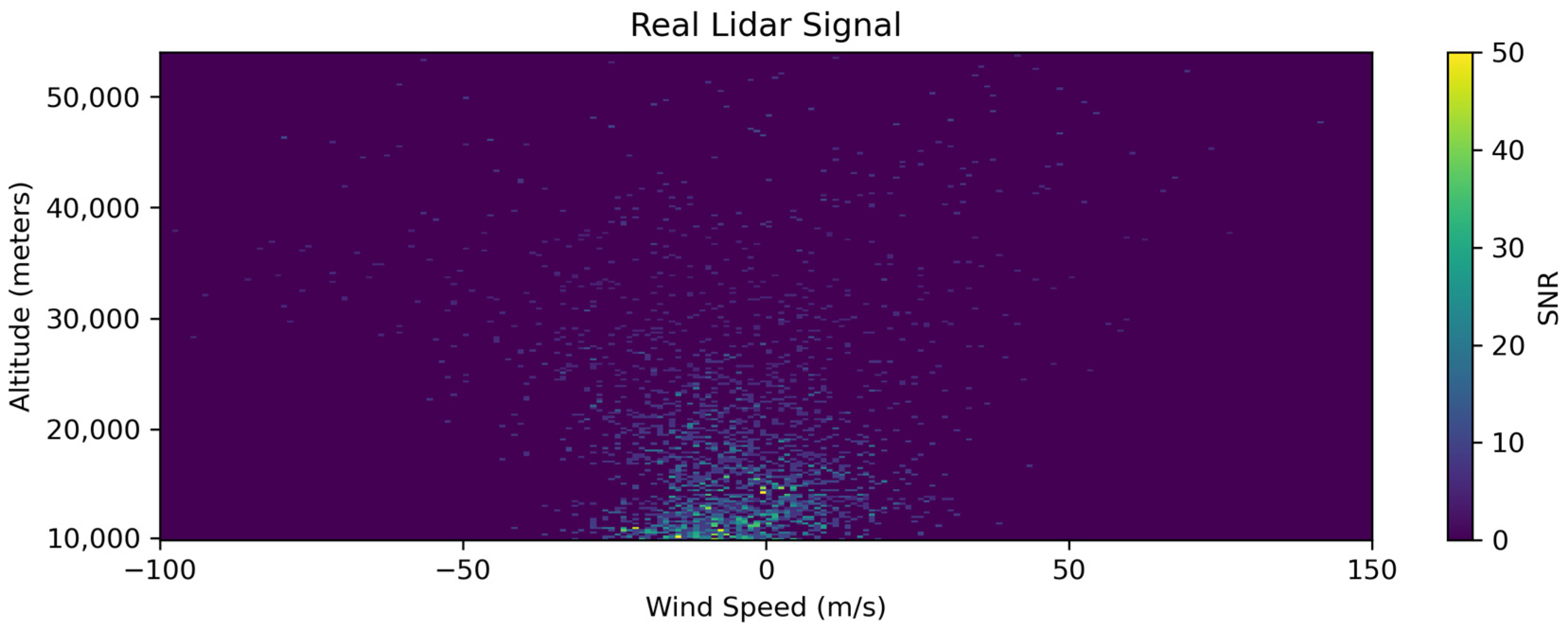
3.1. CNN Outputs
3.2. Wind Profile Evaluation for Simulated Signal
3.2.1. Low SNR Scenario
3.2.2. High SNR (Near Field) and Low SNR (Far Field) Region Reanalysis
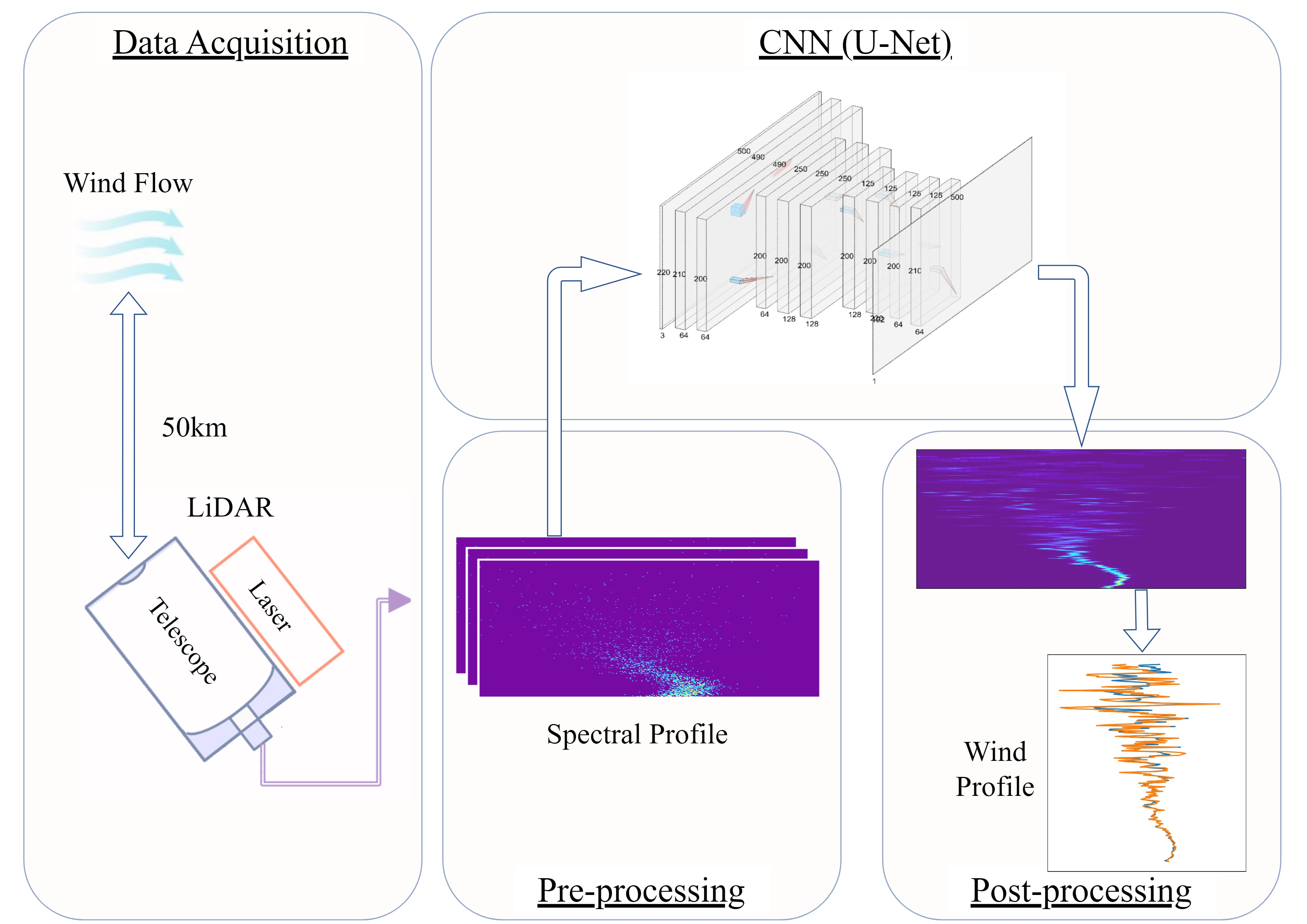
3.3. Wind Profile Evaluation for Real LiDAR Data
4. Discussion
5. Conclusions
Author Contributions
Funding
Data Availability Statement
Acknowledgments
Conflicts of Interest
References
- Krizhevsky, A.; Sutskever, I.; Hinton, G.E. Imagenet classification with deep convolutional neural networks. Adv. Neural Inf. 2012, 60, 1097–1105. [Google Scholar] [CrossRef]
- LeCun, Y.; Bengio, Y.; Hinton, G. Deep learning. Nature 2015, 521, 436–444. [Google Scholar] [CrossRef] [PubMed]
- He, K.Z.; Zhang, X.; Ren, S.; Sun, J. Deep Residual Learning for Image Recognition. In Proceedings of the 2016 IEEE Conference on Computer Vision and Pattern Recognition (CVPR), Las Vegas, NV, USA, 27–30 June 2016; pp. 770–778. [Google Scholar]
- Hu, J.; Shen, L.; Albanie, S.; Sun, G.; Wu, E. Squeeze-and-Excitation Networks. In Proceedings of the IEEE Conference on Computer Vision and Pattern Recognition, Salt Lake City, UT, USA, 18–23 June 2018; pp. 7132–7141. [Google Scholar]
- Iandola, F.N.; Han, S.; Moskewicz, M.W.; Ashraf, K.; Dally, W.J.; Keutzer, K. SqueezeNet: AlexNet-level accuracy with 50x fewer parameters and <0.5 MB model size. arXiv 2016, arXiv:1602.07360. [Google Scholar]
- Howard, A.; Pang, R.; Adam, H.; Le, Q.; Sandler, M.; Chen, B.; Wang, W.; Chen, L.C.; Tan, M.; Chu, G.; et al. Searching for MobileNetV3. In Proceedings of the IEEE/CVF International Conference on Computer Vision, Seoul, Republic of Korea, 27 October–2 November 2019; pp. 1314–1324. [Google Scholar]
- Szegedy, C.; Liu, W.; Jia, Y.; Sermanet, P.; Reed, S.; Anguelov, D.; Erhan, D.; Vanhoucke, V.; Rabinovich, A. Going deeper with convolutions. In Proceedings of the 2015 IEEE Conference on Computer Vision and Pattern Recognition (CVPR), Boston, MA, USA, 7–12 June 2015; pp. 1–9. [Google Scholar]
- Devlin, J.; Chang, M.-W.; Lee, K.; Toutanova, K. BERT: Pre-training of Deep Bidirectional Transformers for Language Understanding. arXiv 2018, arXiv:1810.04805. [Google Scholar]
- Radford, A.; Wu, J.; Child, R.; Luan, D.; Amodei, D.; Sutskever, I. Language models are unsupervised multitask learners. OpenAI Blog 2019, 1, 8. [Google Scholar]
- Brown, T.B.; Mann, B.; Ryder, N.; Subbiah, M.; Kaplan, J.; Dhariwal, P.; Neelakantan, A.; Shyam, P.; Sastry, G.; Askell, A.; et al. Language Models are Few-Shot Learners. Adv. Neural Inf. Process. Syst. 2020, 33, 1877–1901. [Google Scholar]
- Vaswani, A.; Shazeer, N.; Parmar, N.; Uszkoreit, J.; Jones, L.; Gomez, A.N.; Kaiser, Ł.; Polosukhin, I. Attention is all you need. In Proceedings of the Advances in Neural Information Processing Systems, Long Beach, CA, USA, 4–9 December 2017. [Google Scholar]
- Kliebisch, O.; Uittenbosch, H.; Thurn, J.; Mahnke, P. Coherent Doppler wind lidar with real-time wind processing and low signal-to-noise ratio reconstruction based on a convolutional neural network. Opt. Express 2022, 30, 5540–5552. [Google Scholar] [CrossRef] [PubMed]
- Mohandes, M.A.; Rehman, S. Wind Speed Extrapolation Using Machine Learning Methods and LiDAR Measurements. IEEE Access 2018, 6, 77634–77642. [Google Scholar] [CrossRef]
- Song, Y.; Su, Z.; Chen, C.; Sun, D.; Chen, T.; Xue, X. Denoising coherent Doppler lidar data based on a U-Net convolutional neural network. Appl. Opt. 2024, 63, 275–282. [Google Scholar] [CrossRef]
- Huffaker, R.M.; Hardesty, R.M. Remote sensing of atmospheric wind velocities using solid-state and CO2 coherent laser systems. Proc. IEEE 1996, 84, 181–204. [Google Scholar] [CrossRef]
- Huffaker, R.M.; Jelalian, A.V.; Thomson, J.A.L. Laser-Doppler system for detection of aircraft trailing vortices. Proc. IEEE 1970, 58, 322–326. [Google Scholar] [CrossRef]
- Baumgarten, K.; Gerding, M.; Lübken, F.-J. Seasonal variation of gravity wave parameters using different filter methods with daylight lidar measurements at midlatitudes. J. Geophys. Res. Atmos. 2017, 122, 2683–2695. [Google Scholar] [CrossRef]
- Dou, X.; Han, Y.; Sun, D.; Xia, H.; Shu, Z.; Zhao, R.; Shangguan, M.; Guo, J. Mobile Rayleigh Doppler lidar for wind and temperature measurements in the stratosphere and lower mesosphere. Opt. Express 2014, 22, A1203–A1221. [Google Scholar] [CrossRef] [PubMed]
- Chanin, M.L.; Garnier, A.; Hauchecorne, A.; Porteneuve, J. A Doppler lidar for measuring winds in the middle atmosphere. Geophys. Res. Lett. 1989, 16, 1273–1276. [Google Scholar] [CrossRef]
- Besson, A.; Canat, G.; Lombard, L.; Valla, M.; Durécu, A.; Besson, C. Long-range wind monitoring in real time with optimized coherent lidar. Opt. Eng. 2017, 56, 031217. [Google Scholar] [CrossRef]
- Baumgarten, G.; Fiedler, J.; Hildebrand, J.; Lübken, F.J. Inertia gravity wave in the stratosphere and mesosphere observed by Doppler wind and temperature lidar. Geophys. Res. Lett. 2015, 42, 10929–10936. [Google Scholar] [CrossRef]
- Ehard, B.; Kaifler, B.; Kaifler, N.; Rapp, M. Evaluation of methods for gravity wave extraction from middle-atmospheric lidar temperature measurements. Atmos. Meas. Tech. 2015, 8, 4645–4655. [Google Scholar] [CrossRef]
- Yamashita, C.; Chu, X.; Liu, H.L.; Espy, P.J.; Nott, G.J.; Huang, W. Stratospheric gravity wave characteristics and seasonal variations observed by lidar at the South Pole and Rothera, Antarctica. J. Geophys. Res. Atmos. 2009, 114. [Google Scholar] [CrossRef]
- Duck, T.J.; Whiteway, J.A.; Carswell, A.I. The gravity wave–Arctic stratospheric vortex interaction. J. Atmos. Sci. 2001, 58, 3581–3596. [Google Scholar] [CrossRef]
- Chane-Ming, F.; Molinaro, F.; Leveau, J.; Keckhut, P.; Hauchecorne, A. Analysis of gravity waves in the tropical middle atmosphere over La Reunion Island (21 S, 55 E) with lidar using wavelet techniques. Ann. Geophys. 2000, 18, 485–498. [Google Scholar] [CrossRef]
- Mzé, N.; Hauchecorne, A.; Keckhut, P.; Thétis, M. Vertical distribution of gravity wave potential energy from long-term Rayleigh lidar data at a northern middle-latitude site. J. Geophys. Res. Atmos. 2014, 119, 12069–12083. [Google Scholar] [CrossRef]
- Alexander, M.; Geller, M.; McLandress, C.; Polavarapu, S.; Preusse, P.; Sassi, F.; Sato, K.; Eckermann, S.; Ern, M.; Hertzog, A. Recent developments in gravity-wave effects in climate models and the global distribution of gravity-wave momentum flux from observations and models. Q. J. R. Meteorol. Soc. 2010, 136, 1103–1124. [Google Scholar] [CrossRef]
- Flesia, C.; Korb, C.L. Theory of the double-edge molecular technique for Doppler lidar wind measurement. Appl. Opt. 1999, 38, 432–440. [Google Scholar] [CrossRef] [PubMed]
- Ronneberger, O.; Fischer, P.; Brox, T. U-Net: Convolutional Networks for Biomedical Image Segmentation. In Proceedings of the Medical Image Computing and Computer-Assisted Intervention—MICCAI 2015, Munich, Germany, 5–9 October 2015. [Google Scholar] [CrossRef]
- Chen, C.; Zhang, N. Wind Observations of USTC Rayleigh Doppler Lidar in 2019 (Xinjiang); Science Data Bank: Beijing, China, 2022. [Google Scholar] [CrossRef]
- Zhang, N.; Sun, D.; Han, Y.; Chen, C.; Wang, Y.; Zheng, J.; Liu, H.; Han, F.; Zhou, A.; Tang, L. Zero Doppler correction for Fabry–Pérot interferometer-based direct-detection Doppler wind LIDAR. Opt. Eng. 2019, 58, 054101. [Google Scholar] [CrossRef]
- Chen, C.; Xue, X.; Sun, D.; Zhao, R.; Han, Y.; Chen, T.; Liu, H.; Zhao, Y. Comparison of Lower Stratosphere Wind Observations From the USTC’s Rayleigh Doppler Lidar and the ESA’s Satellite Mission Aeolus. Earth Space Sci. 2022, 9, e2021EA002176. [Google Scholar] [CrossRef]
- Chanin, M.L.; Hauchecorne, A. Lidar observation of gravity and tidal waves in the stratosphere and mesosphere. J. Geophys. Res. Ocean. 1981, 86, 9715–9721. [Google Scholar] [CrossRef]
- Garnier, A.; Chanin, M.L. Description of a Doppler rayleigh LIDAR for measuring winds in the middle atmosphere. Appl. Phys. B 1992, 55, 35–40. [Google Scholar] [CrossRef]
- Zhao, R.; Dou, X.; Sun, D.; Xue, X.; Zheng, J.; Han, Y.; Chen, T.; Wang, G.; Zhou, Y. Gravity waves observation of wind field in stratosphere based on a Rayleigh Doppler lidar. Opt. Express 2016, 24, A581–A591. [Google Scholar] [CrossRef] [PubMed]
- Hersbach, H.; Bell, B.; Berrisford, P.; Hirahara, S.; Horányi, A.; Muñoz-Sabater, J.; Nicolas, J.; Peubey, C.; Radu, R.; Schepers, D.; et al. The ERA5 global reanalysis. Q. J. R. Meteorol. Soc. 2022, 146, 1999–2049. [Google Scholar] [CrossRef]
- ERA5: Data Documentation-Copernicus Knowledge Base-ECMWF Confluence Wiki. Available online: https://confluence.ecmwf.int/display/CKB/ERA5%3A+data+documentation#ERA5:datadocumentation-Observations (accessed on 9 March 2023).
- Sun, D.; Zhong, Z.; Zhou, J.; Hu, H.; Kobayashi, T. Accuracy Analysis of the Fabry–Perot Etalon Based Doppler Wind Lidar. Opt. Rev. 2005, 12, 409–414. [Google Scholar] [CrossRef]
- Korb, C.L.; Gentry, B.M.; Weng, C.Y. Edge technique: Theory and application to the lidar measurement of atmospheric wind. Appl. Opt. 1992, 31, 4202–4213. [Google Scholar] [CrossRef]
- Baumgarten, K.; Gerding, M.; Baumgarten, G.; Lübken, F.J. Temporal variability of tidal and gravity waves during a record long 10-day continuous lidar sounding. Atmos. Chem. Phys. 2018, 18, 371–384. [Google Scholar] [CrossRef]
- Senf, F.; Achatz, U. On the impact of middle-atmosphere thermal tides on the propagation and dissipation of gravity waves. J. Geophys. Res. Atmos. 2011, 116. [Google Scholar] [CrossRef]
- Eckermann, S.D.; Marks, C.J. An idealized ray model of gravity wave-tidal interactions. J. Geophys. Res. Atmos. 1996, 101, 21195–21212. [Google Scholar] [CrossRef]
- Alexander, M.; Holton, J. On the spectrum of vertically propagating gravity waves generated by a transient heat source. Atmos. Chem. Phys. 2004, 4, 923–932. [Google Scholar] [CrossRef]
- Holton, J.R. The Influence of Gravity Wave Breaking on the General Circulation of the Middle Atmosphere. J. Atmos. Sci. 1983, 40, 2497–2507. [Google Scholar] [CrossRef]
- Kreyszig, E.; Stroud, K.; Stephenson, G. Advanced engineering mathematics. Integration 2008, 9, 1045. [Google Scholar]
- Vadas, S.L.; Fritts, D.C.; Alexander, M.J. Mechanism for the Generation of Secondary Waves in Wave Breaking Regions. J. Atmos. Sci. 2003, 60, 194–214. [Google Scholar] [CrossRef]
- Andreassen, Ø.; Wasberg, C.E.; Fritts, D.C.; Isler, J.R. Gravity wave breaking in two and three dimensions: 1. Model description and comparison of two-dimensional evolutions. J. Geophys. Res. Atmos. 1994, 99, 8095–8108. [Google Scholar] [CrossRef]
- Fritts, D.C.; Isler, J.R.; Andreassen, Ø. Gravity wave breaking in two and three dimensions: 2. Three-dimensional evolution and instability structure. J. Geophys. Res. Atmos. 1994, 99, 8109–8123. [Google Scholar] [CrossRef]
- Agarap, A.F. Deep Learning using Rectified Linear Units (ReLU). arXiv 2019, arXiv:1803.08375. [Google Scholar]
- Nagi, J.; Ducatelle, F.; Di Caro, G.A.; Ciresan, D.; Meier, U.; Giusti, A.; Nagi, F.; Schmidhuber, J.; Gambardella, L.M. Max-pooling convolutional neural networks for vision-based hand gesture recognition. In Proceedings of the 2011 IEEE International Conference on Signal and Image Processing Applications, ICSIPA 2011, Kuala Lumpur, Malaysia, 16–18 November 2011. [Google Scholar]
- Kingma Diederik, B.J. Adam: A Method for Stochastic Optimization. In Proceedings of the International Conference on Learning Representations, Banff, AB, Canada, 14–16 April 2014. [Google Scholar]
- Zhao, R.; Dou, X.; Xue, X.; Sun, D.; Han, Y.; Chen, C.; Zheng, J.; Li, Z.; Zhou, A.; Han, Y.; et al. Stratosphere and lower mesosphere wind observation and gravity wave activities of the wind field in China using a mobile Rayleigh Doppler lidar. J. Geophys. Res. Space Phys. 2017, 122, 8847–8857. [Google Scholar] [CrossRef]


| Method | Mean | Max. | Min. |
|---|---|---|---|
| AMCNN | 0.0126 | 0.5564 | −0.5051 |
| SCCNN | 0.6141 | 0.8232 | 0.3119 |
| SCR | −0.1680 | 0.5530 | −0.9087 |
| GSSC | 0.4702 | 0.7779 | 0.0241 |
| Time | SCCNN | GSSC |
|---|---|---|
| 31 October, 9:00 p.m. | 0.4536 | 0.3068 |
| 10:00 p.m. | 0.4669 | 0.3676 |
| 11:00 p.m. | 0.3312 | 0.2336 |
| 1 November, 00:00 a.m. | 0.0985 | 0.1552 |
| 1:00 a.m. | −0.0429 | −0.5710 |
| 2:00 a.m. | 0.7653 | 0.6915 |
| 3:00 a.m. | 0.1371 | 0.0010 |
| Mean | 0.3157 | 0.1693 |
Disclaimer/Publisher’s Note: The statements, opinions and data contained in all publications are solely those of the individual author(s) and contributor(s) and not of MDPI and/or the editor(s). MDPI and/or the editor(s) disclaim responsibility for any injury to people or property resulting from any ideas, methods, instructions or products referred to in the content. |
© 2024 by the authors. Licensee MDPI, Basel, Switzerland. This article is an open access article distributed under the terms and conditions of the Creative Commons Attribution (CC BY) license (https://creativecommons.org/licenses/by/4.0/).
Share and Cite
Li, J.; Chen, C.; Han, Y.; Chen, T.; Xue, X.; Liu, H.; Zhang, S.; Yang, J.; Sun, D. Wind Profile Reconstruction Based on Convolutional Neural Network for Incoherent Doppler Wind LiDAR. Remote Sens. 2024, 16, 1473. https://doi.org/10.3390/rs16081473
Li J, Chen C, Han Y, Chen T, Xue X, Liu H, Zhang S, Yang J, Sun D. Wind Profile Reconstruction Based on Convolutional Neural Network for Incoherent Doppler Wind LiDAR. Remote Sensing. 2024; 16(8):1473. https://doi.org/10.3390/rs16081473
Chicago/Turabian StyleLi, Jiawei, Chong Chen, Yuli Han, Tingdi Chen, Xianghui Xue, Hengjia Liu, Shuhua Zhang, Jing Yang, and Dongsong Sun. 2024. "Wind Profile Reconstruction Based on Convolutional Neural Network for Incoherent Doppler Wind LiDAR" Remote Sensing 16, no. 8: 1473. https://doi.org/10.3390/rs16081473