
Kinematic and Dynamic Structure of the 18 May 2020 Squall Line over South Korea

1
Department of Atmospheric Sciences, Center for Atmospheric REmote Sensing, Kyungpook National University, Daegu 41944, Republic of Korea
2
Department of Atmospheric Sciences, Chinese Culture University, Taipei 11114, Taiwan
3
Institute for Earth, Computing, Human and Observing (ECHO), Chapman University, Orange, CA 92866, USA
*
Author to whom correspondence should be addressed.
Remote Sens. 2024, 16(8), 1474; https://doi.org/10.3390/rs16081474
Submission received: 16 February 2024
/
Revised: 1 April 2024
/
Accepted: 13 April 2024
/
Published: 22 April 2024
(This article belongs to the Section Atmospheric Remote Sensing)
Abstract
:The diagonal squall line that passed through the Korean Peninsula on the 18 May 2020 was examined using wind data retrieved from multiple Doppler radar synthesis focusing on its kinematic and dynamic aspects. The low-level jet, along with warm and moist air in the lower level, served as the primary source of moisture supply during the initiation and formation process. The presence of a cold pool accompanying the squall line played a role in retaining moisture at the surface. As the squall line approached the Korean Peninsula, the convective bands in the northern segment (NS) and southern segment (SS) of the squall line exhibited distinct evolutionary patterns. The vertical wind shear in the NS area was more pronounced compared to that in the SS. The ascending inflow associated with the tilted updraft in the NS reached an altitude of 7 km, whereas it was only up to 4 km in the SS. The difference was caused by the strong descending rear flow, which obstructed the ascending inflow and let to significant updraft in the SS.
1. Introduction
Mesoscale linear convective systems, known as squall lines or quasi-linear convective systems (QLCSs), exhibit a notable organization and longevity, spanning in a horizontal range of 20 to 200 km and persisting for several hours. They have the capacity to generate various severe conditions, including tornadoes, thunderstorms, strong winds, hail, heavy precipitation, and other potentially catastrophic weather events [1,2,3,4,5]. Nowadays, the frequency and intensity of robust convective weather events have experienced a discernible surge. This escalation presents a substantial threat to the daily lives of those inhabiting regions affected by such events [6]. Understanding the interconnection of severe weather and its multifaceted impact on lives, economies, and the environment [7] underscores the importance of proactive measures in disaster preparedness, response, and recovery.
The structure of a squall line is influenced by various factors, including atmospheric stability, moisture availability, wind shear, topography, and synoptic-scale weather patterns [8,9]. Synoptic-scale weather patterns, exemplified by the existence of frontal systems or upper-level disturbances, can influence the arrangement and duration of squall lines. These expansive features generate the favorable conditions for the initiation and sustenance of squall lines. Subsequently, examining the impact of environmental wind shear becomes crucial for understanding squall line dynamics [4,9,10]. An environment with pronounced wind shear at the leading edge is important in creating the necessary conditions for storms to organize efficiently, maintain longevity, and potentially escalate into severe weather systems [4,8,9,10,11,12]. Additionally, the presence of a cold pool at the surface strengthens the development and duration of the system [9,13,14] emerging as a fundamental determinant in the intricate dynamics of squall line development. A prominent cold pool and topography among the various convective forces, resulting from processes such as precipitation evaporation or water loading, repeatedly triggers the initiation of convection development [15,16,17].
Previous studies have extensively examined the structure of mid-latitude squall lines [18,19,20,21]. The precise structure and characteristics of mid-latitude squall lines can vary depending on atmospheric conditions, geographical location, and other contributing factors. Utilizing three-dimensional radar reflectivity proves essential in depicting the intricate structure of these squall lines [19,20,22]. This method aids in studying the life cycle of the system, along with analyzing its convective and stratiform regions. Refs. [11,23] identified updrafts in the convective area, which interacts with incoming moist environmental air near the leading edge. Typically, the updraft tilts backward and extends into upper levels along the stratiform region. Ref. [24] pointed out that the structural features of squall lines in the northwest of Taiwan exhibited similarities with the general feature of squall lines. Across the frontal side, there was prevailing front-to-rear flow at all altitudes, coupled with shallow rear-to-front flow on the opposite side. Additionally, convective downdrafts were observed trailing behind the main cells [14].
The utilization of radar composites is important for convective system propagation. Ref. [25] identified the significant portion of stratiform precipitation during convective systems in the West Africa. Additionally, the result also indicated the region with the rainfall production from the propagating convection system. The radar composite is also a good starting point to depict how the convection system evolves. High-resolution reflectivity analyses can also be essential features in the process of assimilating data into convective-scale numerical weather models over extensive geographic domains [26]. Since the weather radar can provide high temporal and spatial observation data, some studies regarding convection system mechanism and structure have been conducted [21,23,24,27]. To observe the kinematic characteristics of the convection system, retrieval of winds from multiple Doppler radar synthesis is carried out [28]. Recently, a new scheme of synthesis of retrieved winds was employed to undertake a comprehensive analysis of three-dimensional precipitation and wind fields over the topography in Pyeongchang, Republic of Korea [29]. It is integrated with the radar measurement, sounding, model forecasts, and additional sources, such as the surface observation.
The importance of Automatic Weather Stations (AWSs) in depicting the change in surface parameters should be considered in the analysis. The Korea Meteorological Administration (KMA) manages an extensive surface observational network that includes AWSs in Republic of Korea. Ref. [30] systematically characterized the surface properties of the cold pool within the region influenced by the MCS. The investigation revealed that the existence of the cold pool was a significant factor influencing alterations in various surface parameters. The cold pool’s presence exhibited a discernible impact on the local surface conditions, leading to noteworthy changes in the studied parameters.
The study employs an analysis technique that involves utilizing soundings to investigate the environmental sounding. Ref. [31] examined a sounding released ~4 km ahead of the squall line gust front, revealing the presence of a moist unstable layer within a rapidly ascending environment. Furthermore, as the squall line moved towards the sites of the sounding, there was a noticeable increase in both low-level and deep-layer vertical wind shear measurements. This underscores the dynamic changes in atmospheric conditions associated with the squall line’s development.
Considering that most of the recent research focuses on the model simulation of squall lines, it is useful to obtain the information of the squall line structure from high-resolution observation data. Therefore, this study focused on the development and structure of a diagonal squall line that occurred in the Korean Peninsula on 18 May 2020 using retrieved winds from multiple Doppler radar synthesis. Despite notable advancements in comprehending the kinematic and dynamic structure of squall lines, further study is still needed to provide a more detailed examination of the complex structural features inherent in the squall lines, especially the characteristics of segments. In this paper, we analyzed the event by analyzing the large-scale weather pattern to observe how the system initiated, revealing the environmental factor that influenced the system structure, and enabling us to examine the kinematic and dynamic features along the segments in squall lines to identify the distinct structure in different geographical locations (such as ocean, coast, and inland).
The subsequent sections of the paper are structured as follows: Section 2 presents the data sources and analysis procedures. Section 3 presents the case overview, including the evolution process and movement of the squall line. Section 4 articulates our findings regarding comprehensive analysis from kinematic and dynamic perspectives, and a concise summary and additional discussion are presented in Section 5.
2. Data Sources and Analysis Procedures
2.1. Data Sources
The study focused on analyzing a specific occurrence of a diagonal squall line that occurred in the transitional period between spring and summer. The KMA operates S-band dual-polarization radars that provide the radar reflectivity field (Z). The horizontal and vertical resolution of the data are 500 m and 50 m, respectively. For further details on the locations, scanning strategies, and specifications of these radars, refer to [32,33]. The Wind Synthesis System Using Doppler Measurements (WISSDOM) is employed to represent the wind field component, and its application in the Korea region has been documented by [29]. WISSDOM is known for providing optimal wind information, offering a more precise depiction of the flow field over varied topography. This dataset includes estimates of horizontal and vertical wind components, as well as vorticity and divergence, with a horizontal grid resolution of 1 km and a vertical resolution spanning from 0 to 10 km altitude. For further details on WISSDOM, refer to [29].
Radiosonde observations are used to provide concise details about the environmental conditions in the vertical profile over specific layers. The outcomes of these observations serve to characterize the upper air state in the vicinity by selecting two stations closely situated to the convective system formation location, namely Baekryeongdo (47102) and Osan (47122). Observations at these stations are conducted twice daily at 0000 UTC (09:00 LST) and 1200 UTC (21:00 LST). In this particular case study, selected time was directed towards 0000 UTC (3 h prior to the system occurrence), given that the convection system initiated in the early afternoon. The study calculated radiosonde parameters, which include temperature, dew point, pressure, and wind profile, to determine Convective Available Potential Energy (CAPE) and bulk wind shear. Ref. [34] employed both parameters as a reliable method for distinguishing between severe thunderstorms of significant impact and those of lesser severity. Surface meteorological observations from 969 KMA Automatic Weather Stations (AWSs) are essential datasets for discerning the presence of a cold pool at the surface. Selecting parameters from the Incheon and Seoul stations, including precipitation, surface pressure, wind, and equivalent potential temperature [35], was anticipated to assist in conducting surface analysis.
2.2. Analysis Procedures
The research area for this study encompasses a significant portion of the Korean mainland, as illustrated in Figure 1, spanning coordinates 124 130°E and 34 38.5°N. The Korean mainland is known for its mountainous terrain, with the Taebaek Mountains extending down the eastern side and the Sobaek Mountains to the south. Meanwhile, the western and southern coasts are the location of the majority of coastal plains. The selection of this study area aligns with the geographic extent of the data to assess the relative importance of radar variables. The chosen region of interest facilitates a comprehensive examination of the system’s morphology, and it allows for the utilization of gridded AWS observations to depict the spatial distribution to support the analysis. The kinematic and dynamic result is examined through a vertical cross-section in each selected time at different stages, which represent geographical location (over ocean, coastal, and inland), shown in Figure 1. The area of analysis was divided into two segments along 125 128.5°E for each with the criteria: one is the northern segment (NS), which covers an area of 36.5 38°N, and the other is the southern segment (SS), which covers an area of 35 36.5°N.
The investigation into the spatial distribution and evolution of the squall line involves utilizing the Constant-Altitude Plan Position Indicator (CAPPI) product obtained from S-band composite radars. After selecting the specific case under examination, the squall lines diagonally traversing the Korean mainland were manually identified. Reflectivity (Z) datasets were examined to recognize squall line patterns based on previously criteria defined [2]. The criteria include identifying continuous areas where reflectivity values reach or exceed 40 dBZ, spanning a minimum range of 100 km and lasting less than 3 h. The ideal reflectivity area exhibits a frequently observed leading edge and a linear shape at 40 dBZ. Based on the previously described criteria, this study aimed to show how the squall line evolves and propagates by depicting the hourly reflectivity in the zonal distribution.
The calculation of the squall line’s movement was scrutinized to ascertain a nearly constant speed and direction. Determining storm motion allows the estimation of the storm’s heading with a velocity close to that of the mean wind over the storm’s depth. In terms of storm motion, calculations were performed to track the primary convective band within the line and its propagation due to the triggering of new convective bands. It is important to note that the average storm motion is determined by the environmental wind, assuming no external forcing. Environmental wind calculations span from near-surface to 6 km altitudes [36], with increments having a height of 200 m. Storm-relative winds are then calculated by directly subtracting storm motion from environmental winds at each of the aforementioned heights [37], using the following formula below:
where is storm-relative winds (,w), is environmental winds, is the storm motion, and units are in m s−1. Utilizing WISSDOM, the vertical wind shear can be calculated by examining the spatial and temporal variations of u and v wind components between near-surface and 3 km altitudes.
The temperature () and pressure () from AWS data are used at each site to determine the equivalent potential temperature (), as the following formula below:
where is a reference pressure (1000 hPa), is the gas constant for dry air (287 J kg−1 K−1), and is the specific heat capacity of dry air at constant pressure (1005 J kg−1 K−1). For each spatial point, the calculation of the perturbation of equivalent potential temperature () can be defined as:
where is the reference equivalent potential temperature, obtained from the average value of at particular time.
3. A Case Overview
3.1. Evolution of Squall Line
The composite radar reflectivity reveals the evolution of the squall line, showing some single convective bands with reflectivity exceeding 35 dBZ over the Yellow Sea (the western part of the Korea mainland) in Figure 2a (stage I). The early developed bands were shown at around 0400 UTC, and showed a cluster-like distribution and back-building convective storm characteristics. The process occurred as a new convective band formed in the southern portion and interacted with the pre-existing band. This interaction caused the squall line to develop in a backward pattern, where a new convective band eventually formed behind the early developed convective system, merged with the older convective band ahead, and consequently expanded the convection area.
From 0400 to 0500 UTC, the system was in the developing stage, with the convective band continuing to propagate eastward and intensify. Figure 2b illustrates the mature stage, where the system intensified and evolved into a squall line at 0500 UTC, as seen in domains I and IV. The radar reflectivity showed a well-defined narrow band oriented in the northeast–southwest direction, propagating eastward with a dense reflectivity contour and well-defined structure. The strong convective band showed a maximum reflectivity of 62 dBZ and continued to intensify as it moved toward the mainland. By 0600 UTC, the squall line had reached the mainland via the NS (domain II), while the SS of the squall line remained over domain IV, as shown in Figure 2c. In the following hour, initial fragmentation within the SS was observed at the boundary between domains IV and V. During this time, squall line had an asymmetric structure, with a broad northern part and a narrower, more fractured southern part (Figure 2d).
Figure 2e,f reveal the prominent broken structure in the SS as the system approached the coastline (domain V). Meanwhile, the convective band in the NS maintained its structure, having already reached domain III (inland). The propagation of the convective band in the NS was faster than that in the SS. During the dissipation stage from 1000 UTC, the convective band structure in the NS exhibited a comma pattern with an observed reflectivity of 45 dBZ, extending beyond the boundary of domain III (Figure 2g). In contrast, the convective band in the SS exhibited a broken pattern with multiple discrete convective bands within domain V. By the time 1100 UTC, the dissipation stage of the squall line became distinctly evident for both NS and SS. The reflectivity distribution showed a discernible decrease, signifying a decline in convective activity within the squall line.
3.2. Movement of Squall Line
Figure 3a illustrates the trajectory of the leading edge of the squall line throughout the observational period, spanning from 0400 to 0920 UTC. It shows the location of the leading edge represented by the 35 dBZ contour, using a series of 2 km reflectivity data collected during this time frame. The primary objective of this movement was to understand the squall line’s progression from its initiation area to the mainland. The squall line’s directional movement is highlighted by arrows in Figure 3a, indicating the movement vectors and the leading edge’s trajectory over time. The highest speed recorded was 12.41 m s−1 between 0500 to 0600 UTC, illustrating the rapid advance of the leading edge from the ocean towards the coastline. Overall, from 0400 to 1100 UTC, the leading edge of the squall line showed an eastward movement with varying speeds, and the slowest was observed at 11:00 UTC during the system’s dissipation phase.
The reflectivity greater than 35 dBZ over time shows the spatial and temporal evolution of the squall line (Figure 3b). At 0500 UTC, the squall line reached its maximum length of approximately 367.4 km, indicating that the system was in its mature stage over the ocean. In the NS, the convective band maintained its structure and continued its eastward movement, while in the SS it began showing a fractured structure from 0700 UTC. Reflectivity greater than 35 dBZ persisted in the NS up to the dissipation stage at 1100 UTC. In contrast, as the squall line approached the mainland in the SS around 0800 UTC, the region having greater than 35 dBZ had already disappeared. Figure 3c presents the time series analysis correlating the mean reflectivity with the area greater than 35 dBZ. The analysis begins at 0300 UTC when the convective band initiated with the mean reflectivity at 30 dBZ and a relatively small area under 8000 km2. As the convective band progressed into the development stage around 0400 UTC, a gradual increase in mean reflectivity to 33 dBZ was observed. The most significant change of the pattern observed during the mature stage (0500 0600 UTC) over the ocean and coast, showcasing a peak mean reflectivity of approximately 38 dBZ. This aligns seamlessly with a considerable expansion of the area of between 14,000 and 16,000 km2. Following the squall line’s arrival on the mainland by 0700 UTC, both mean reflectivity and the corresponding area exhibited a decline, indicating the influence of complex terrain.
However, a noteworthy deviation occurred around 0800 UTC, marked by a subtle increase in both mean reflectivity and area. This can be attributed to the sustained deep convective structure in the NS, which persisted despite the fragmentation structure in the SS, lasting until 0920 UTC. After 0920 UTC, a discernible decline in reflectivity suggested the weakening of convective activities in the squall line during the dissipation stage. Throughout the observation period, Figure 3c consistently demonstrates a positive correlation between the mean reflectivity and the area, highlighting the interdependence of these two parameters in illustrating the evolving dynamics of the squall line. An interesting observation during the development stage is that the area of the squall line expanded before an increase in mean reflectivity was noted. However, a decline in reflectivity occurred prior to any reduction in the area, aligning with expectations given the squall line’s convective structure. Yet, in the final phase of this specific squall line, the area started to contract before any decrease in convective strength was detected. This indicates the dissipation of the convective region in the SS, accompanied by a re-intensification in the convective line of the NS.
4. Comprehensive Analysis of Squall Line Dynamics and Environmental Influences
4.1. Synoptic-Scale Weather Pattern
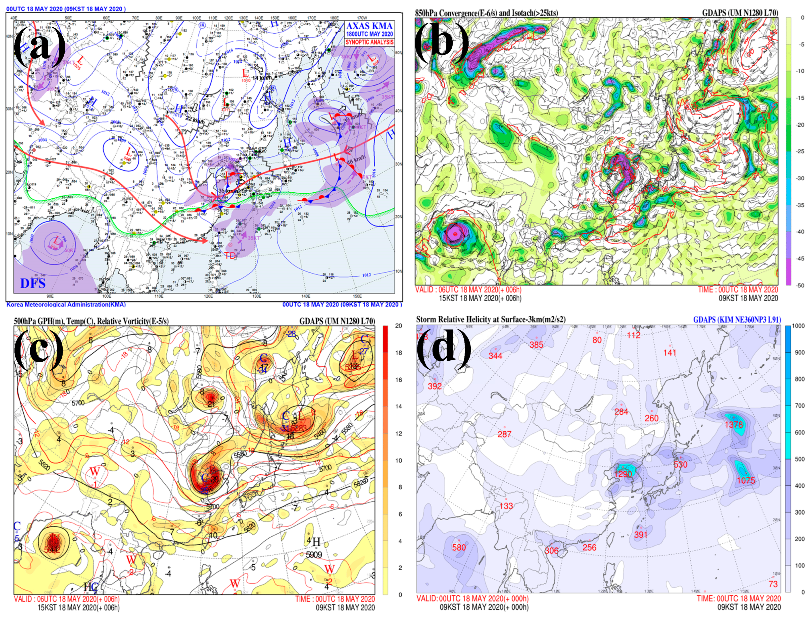
The synoptic conditions preceding the squall line formation are visually represented in Figure 4. The figure provides a comprehensive overview of the atmospheric conditions and large-scale weather patterns leading up to the initiation of the squall line. The surface weather map indicates the presence of a low-pressure system (LPS) over mainland China, moving eastward with a center sea level pressure of 997 hPa at 0000 UTC (Figure 4a). The weak stationary fronts and strong eastward-moving jet at 30 knots were also observed at the lower levels. The presence of LPS at the surface was linked with warm and humid conditions due to the convergence zone (Figure 4b), facilitating the influx of warm and moist air, which is crucial for the initiation of the convection system. The convergence area signifies a substantial influx of the amount of water vapor, serving as the primary source for moisture for the developing convective systems. The convergence of moist air in the lower troposphere, supported by both jet streams and the convergence zone, created favorable conditions for convective initiation, with the first convective band forming within this area, indicated by the purple shading.
The synoptic pattern at 500 hPa showed a deep trough over mainland China, associated with the area of larger positive vorticity (20 × 10−5 s−1), as shown in Figure 4c. This feature likely caused the convection that developed in the afternoon over the Yellow Sea. This deep trough formed close to the convection system’s initial location at 0000 UTC and became more pronounced by 0400 UTC, aiding in the uplift of warm and moist air and the subsequent formation of the convection system. Low vortexes and the development of convection systems are favored by an environment with a high storm-relative helicity (SRH) [38]. The higher SRH showed up in the convergence zone and LPS at 0000 UTC, contributing to the upward motion and created lifting mechanisms (Figure 4d). Additionally, a high SRH indicated a wind shear condition that is favorable to the creation of a convection system [39]. Such synoptic conditions played an important role in fostering an unstable atmosphere with significant large-scale vertical motion, creating an environment ripe for convection.
4.2. Upper Air Sounding Analysis
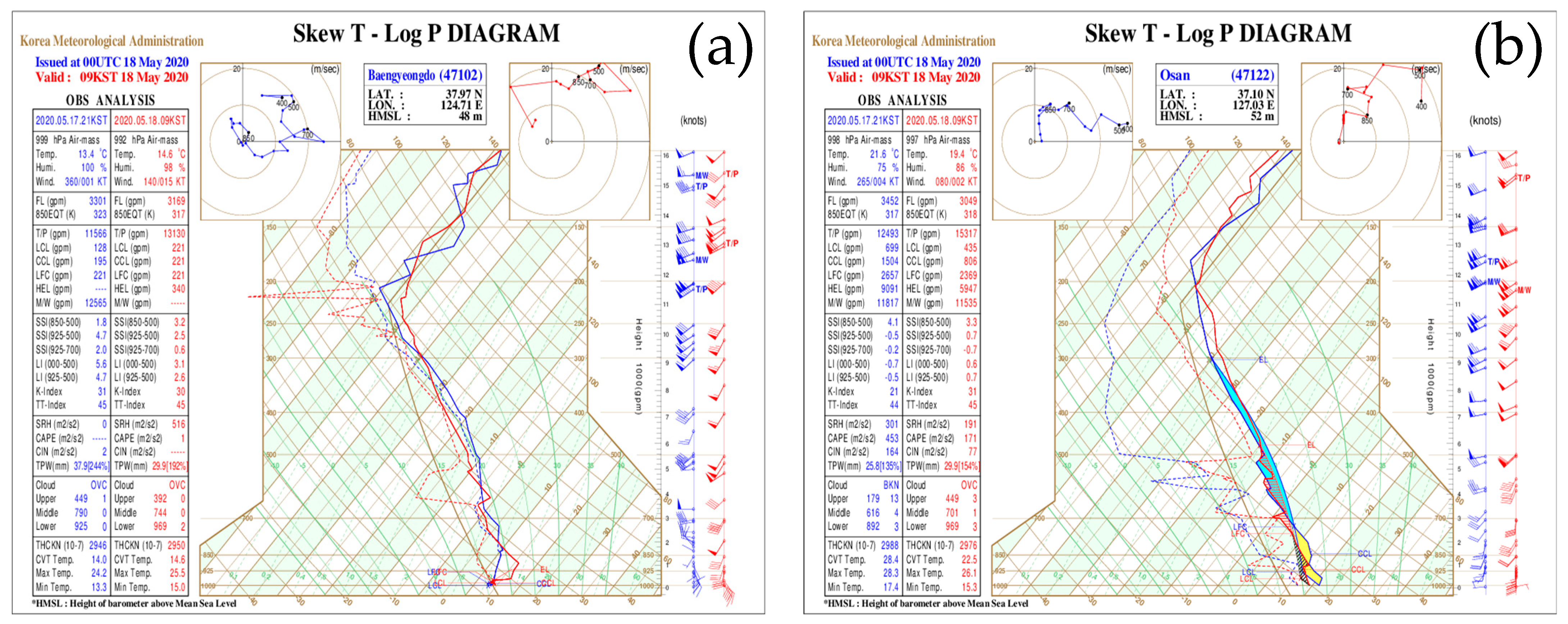
Radiosonde observations at Baekryeongdo and Osan sites were examined to investigate upper air conditions, as shown in Table 1. This sounding was specifically chosen to examine the thermodynamic and kinematic profiles preceding the formation of the convection system. Table 1 provides the information on observed bulk shear 0 6 km () values which exceed 18 m s−1, with the highest value recorded at Osan, reaching 30.9 m s−1. The increase in bulk shear is indicative of the significant vertical wind shear (see Figure 5). The conditions observed at these sounding sites were favorable for the formation of the convection system.
The thermodynamic profile prior to the convection system’s formation was taken at 0000 UTC on 18 May 2020, as shown in Figure 5. The observations from the sites showed the warm air above the 950 hPa level. At the Baekryeongdo site, both the level of free convection (LFC) and equilibrium level (EL) were observed to be around 925 hPa. In contrast, at Osan sites, the values of LFC and EL were about 730 hPa and 475 hPa, respectively. Notably, the LFC was relatively low at Baekryeongdo, whereas at Osan, it was significantly higher. However, the magnitude of Convective Available Potential Energy (CAPE) at both sites was recorded below 200 J kg−1, which was considerably lower than the CAPE values associated with squall line environments in previous studies, which typically exceeded 1200 1500 J kg−1 [3]. Despite these low CAPE values, convective weather events can still occur within an unstable atmospheric environment, which is often characterized by warm (dry) air at the low (middle) altitudes. This condition aligns with the large-scale weather pattern.
4.3. Cold Pool Characteristics
The spatial distribution perturbation of equivalent potential temperature obtained from AWS on 18 May 2020 is illustrated in Figure 6. The presence of a cold pool is inferred from the equivalent potential temperature, pressure, and surface wind field. Prior to the squall line reaching the mainland around 0600 UTC, the equivalent potential temperature exhibited positive values, indicating the presence of warm and moist air at the surface [40]. As the squall line moved near to the coast, there was a decrease in the equivalent potential temperature, as marked by the areas of blue shading. Concurrently, the depiction of reflectivity greater than 35 dBZ is outlined by the green shaded contour. The leading edge was depicted by the thick dashed line, which is located ahead of the reflectivity area. The gradual decrease in equivalent potential temperature indicated the expansion of a cold pool near surface. As seen in Figure 6, the cold pool strengthened and expanded southward after 0700 UTC.
Figure 7 illustrates the change in surface parameters recorded at the Incheon and Seoul weather stations. Initially, the equivalent potential temperature values remained in the positive values. However, a noteworthy shift occurred at the Incheon site, with a value of −8 K dropped in equivalent potential temperature observed around 0610 UTC, coinciding with the squall line nearing the coast. Within the next 40 min, by 0650 UTC, the Seoul site also experienced a sharp decrease in equivalent potential temperature of −6 K. Before the arrival of the squall line, the wind remained as a relatively steady southeasterly flow at around 3 5 m s−1. As the squall line arrived on the mainland, the wind direction shifted westerly at both locations and became calmer. Pressure perturbation showed with a gradual increase at both sites after the squall line’s arrival, with values rising by approximately 2 3 hPa. As the squall line reached the Incheon site, precipitation started at 0620 UTC, peaking at approximately 60.6 mm h−1 around 0630 UTC. Subsequently, the precipitation gradually decreased at a slower rate. Similarly, in the Seoul site, precipitation occurred 30 min later by starting at 0650 UTC with a value of 3 mm h−1. The peak value of 51 mm h−1 was observed at around 0710 UTC; that is, the heavy precipitation started as the squall line reached the sites, and transitioned into moderate or light precipitation when the squall line propagated away.
The strengthening of the cold pool contributed to the concentration of precipitation within a specific area [41]. The condition showed the existence of the cold pool resulting from evaporation cooling, whereas it contributed to maintaining the near-surface equivalent potential temperature and preserving moisture for convection.
4.4. Vertical Wind Shear
Figure 8 shows the spatial distribution of vertical wind shear and its significant variations, highlighting its distinct effects on different segments of the squall line. The figure focuses on the shear pattern in the front of the leading edge (red dashed line). The fast-moving squall line is associated with the development of strong vertical wind shear along its leading edge, affecting the organization of convective cells and the overall structure of the squall line [4,8].
At 0400 UTC, the higher vertical wind shear was apparently observed in front of the leading edge, extending eastward. The highest shear was seen at domain I in the NS and approximately reached 45 m s−1, aligning closely with the leading edge. In a higher shear environment, it is often associated with the reinforcing effects of the rear-inflow jet at the leading edge [42]. During the mature stage at 0500 UTC, the higher shear was clearly seen at domain II and the direction shear remained to the east (Figure 8b). At this time, the weaker shear was observed at the rear of the leading edge. During the propagation to the mainland, the vertical wind shear showed a decrease compared to the vertical shear over the ocean. This reduction became more apparent by 0700 UTC as the squall line made landfall. At this point, the shear’s influence appeared less pronounced across both segments, indicating a diminishing role of shear in the squall line’s dynamics as it progressed inland.
The increase in lower-level vertical wind shear leads to the vertically erected convective cells [42]. The condition will shape the structure of vertical motion at the leading edge, and, consequently, the overall structure of the squall line. While this study does not demonstrate a significant difference between the vertical shear pattern in the NS and SS, the observed case offers the important role of moderate to strong shear in sustaining the squall line’s longevity [8].
4.5. Vertical Structure of the Squall Line
4.5.1. Characteristics of the Squall Line in the Northern Segment
The initial analysis at 0500 UTC focuses on the convective band over the domain I (over the ocean), where a relatively narrow band of high reflectivity reached 35 dBZ. Figure 9a shows the storm-relative flow at 2 km altitudes, and indicates a southerly flow in the front of convective band. This indicates a substantial inward movement of air toward the convective system. In the rear part of the convective band, a strong westerly storm-relative flow was observed. At this stage, the estimation speed of the convective band was ~9.62 m s−1 slower than the typical squall line’s propagation speed in the previous research (~15.5 m s−1) [24].
At 0610 UTC in domain II (Figure 9b), a predominant southeasterly flow was observed, with the inflow pattern shifting as the system approached the coast. In the northern portion of the rear part of the primary convective band, the flow transitioned to westerly and converged with the few southeasterly outflows from the band, while a predominated westerly flow was located in the southern portion. The leading edge featured a stratiform area, although it was narrower than those observed in other squall line cases [2,3,4]. The last observation at 0920 UTC in domain III revealed a prevailing easterly inflow over the inland region (Figure 9c). The primary storm-relative winds were easterly upstream of the convective band, followed by a weakened flow to the rear. Compared to previous stages, the easterly flow at the rear was less pronounced during the dissipation stage.
A vertical cross-section in the NS (domains I, II, and III) was examined to depict the vertical structure of the squall line (Figure 10a f). At stage I, the convective band displayed significant reflectivity, with the 35 dBZ contour reaching heights up to approximately 8 km within the main band (Figure 10a), which is significantly higher than in the previous research [43]. There was a significant ascending front-to-rear flow that peaked at a velocity of 24.2 m s−1 below 4 km (Figure 10d). Such a strong inflow observed at the lower altitudes is crucial for the development and maintenance of a convective system [23], particularly during the mature stage as it approaches the mainland. In particular, in domain I, an elevated rear-to-front flow was noticeable and pronounced at 4 km (middle altitude) upwards. Concurrently, a strong frontward outflow was evident at higher altitude.
The dominant airflow pattern when the squall line arrived at the coastal line (domain II) exhibited the front-to-rear flow ascending to 8 km in altitude (see Figure 10e). A rearward-tilted main front-to-rear flow was observed at this period, with a decrease in reflectivity in the convective region. Although the 35 dBZ contour extended up to 8 km, similar to domain I, the 45 dBZ was reached up to 4 km in altitude and was considerably broader than domain I (Figure 10b). At this domain, the pronounced descending rear-to-front flow was observed from mid to low altitudes [44], maintaining the squall line activity. A narrow stratiform region was observed at the upstream region. Storm-relative flow during domain II showed noticeable differences compared to domain I, particularly in the tilted front-to-rear flow, which is in a good agreement with findings from previous studies [1,2,3,15]. Overturning flow at the convective region produced a gentle downdraft at the mid-level, and this created the stratiform convection in the upstream region.
At 0920 UTC, domain III provided the information on the convective band from observations over the inland (Figure 10c). The vertical extent of reflectivity maintained its structure, and the stratiform region expanded compared to the earlier stage. The reflectivity was much weaker, with a narrow band of 35 dBZ extending only up to 4 km. The stratiform region appeared in downstream, and the rear-to-front descending flow became more pronounced and expanded. Figure 10f showed that the front-to-rear ascending inflow was stronger in the middle altitude with intensities up to 15 m s−1. This enhancement of the front-to-rear flow in the convective region may be attributed to orographic lifting.
4.5.2. Characteristics of the Squall Line in the Southern Segment
In the SS, the initial analysis was examined at 0530 UTC (domain IV), where the presence of the first convective band occurred with noticeable fragmented cells (Figure 11a). Similar to the case of domain I, Figure 11a indicates the presence of a southeasterly flow in the upstream region of the convective band, which was stronger from the coast but much weaker near to the convective band. The northwesterly flow pattern was consistent, extending to the rear part of the convective band, and was much stronger in the north portion. The convective region was much narrower compared to domain I.
Domain V showed the storm-relative flows, and it was similar to domain IV over the ocean. The predominant northerly flow was dominated to the rear part (Figure 11b). A strong southeasterly from the coast was observed in the front of the convective band. By the time the convective band reached the coast, the reflectivity structure appeared fragmented and weakened, marking a clear difference from the more intact structure observed during domain II. By this point, there was a clear difference between domains II and V in the convective band reaching the coast, with the convective band still maintaining its structure at domain II. This distinction underscores the significant structural changes the convective band underwent by domain V upon approaching the coast, in contrast to its maintained integrity at domain II.
The pattern at 1050 UTC displayed only minor differences from earlier domains (see Figure 11c), with a predominantly southeasterly flow along the convective bands. It was evident that the structure of the convective band had already broken and dispersed. Unlike the flow pattern at domains IV and V, there was no deflection pattern flow over domain VI. This change, characterized by the broken structure and the absence of deflection flow, may be associated with local factors, including topography. Topographic features such as mountains can act as barriers to or channels for airflow. Topographic features can affect the airflow dynamics within a squall line. When encountering the terrain, the squall line may be forced to ascend up-slope or descend down-slope, altering its convective behavior and potentially causing fragmentation or breakage in its structure.
Figure 12a–c reveal that the band structure in domains IV VI was relatively narrower compared to in domains I III, which the reflectivity band region expanded. Domain IV showed that the 35 dBZ reflectivity contour of the convective band reached a height of 9 km on the inner side, which was much higher compared to that of domain I (Figure 12a). Domains V and VI showed the similarities in the vertical reflectivity of the convective band. At these domains, the structure revealed a fragmented structure and weakened in reflectivity. Domain V displayed the narrower 35 dBZ reflectivity, predominantly reaching up to 6 km (Figure 12b). In contrast, the reflectivity feature at domain VI was less pronounced, aligning with the dissipation stage (Figure 12c).
The ascending front-to-rear flow reached 6 km in altitude with a value of 15 m s−1, which was significantly weaker than in domain I (Figure 12d). In both stages, the erected front-to-rear flow contributed to the reflectivity reaching higher altitudes. Additionally, the overturning forward outflow was clearly seen from the middle altitudes with a velocity of 25 m s−1. Domains V and VI showed a similar pattern of ascending front-to-rear flow. The pattern showed the flow predominated and only reached a height having a 4 km altitude with a velocity of 10 m s−1. The ascending front-to-rear flow over these domains was noticeably weaker compared to in domains II and III. The reduced strength of storm-relative inflow implies that the warm and moist air, driving the convective activity in the squall line, was restricted.
A significantly elevated rear-to-front flow was prominent in the downstream region of the squall line in domains V and VI (Figure 12e,f). In domain V, the shallow rear inflow was observed below the 2 km altitude, which was relative to the leading edge of the surface cold pool. The presence of terrain features impacting the rear-to-front flow was unlikely to descend to low altitude. Domain VI showed there was no evidence of a descending rear-to-front flow and the ascent of the front-to-rear flow was insignificant, whereas it was weaker than for the ocean and coast. The presence of a strong elevated rear-to-front flow and overturning outflow at these domains demonstrated the system’s behavior toward a less organized structure [4,8].
4.5.3. Vertical Motion Dynamic in the Northern Segment
Figure 13 shows the horizontal distribution of vertical motion over domains I, II and III. The results reveal that a prominent line of updraft (red shading) was observed ahead of the leading edge (black dashed line), fostering convective growth [2,4,8]. The strong updraft reaching to 9 m s−1 at the domain played a crucial role in enhancing convective activity, particularly during the intensification. In contrast, the updraft in domains II and III was much weaker.
The presence of positive vorticity (black line contour) with the updraft line was consistently observed across these domains, indicating a conducive environment for convective development [45]. Wider downdrafts appeared during domain II, when the convective band was near to the coast (Figure 13b). The prominent line of downdraft was observed behind the line of updraft at this stage. Although the downdraft was not much stronger compared to domain I, its spatial extent was more significant at domain II. Domain III continued this trend, with the wider area of downdraft behind the line of updraft (Figure 13c) contributing to the convective band’s structural weakening and eventual dissipation.
Figure 14 illustrates the vertical motion dynamics within the vertical structure for each domain. Figure 14a shows the broad area of updraft associated with the positive vorticity; this facilitated the ascending inflow which reached approximately 8 km at domain I (see Figure 10d). The structure exhibited narrower features during its mature stage, followed by a significant second updraft at the leading edge which was caused by the prominence of vertical wind shear [46], also associated with positive vorticity. The updrafts and downdrafts at domain II showed a similar pattern to those in domain III (Figure 14b,c).
In domain II, the rearward-tilted updraft reached up to 9 km, aligning with the tilted front-to-rear ascending flow observed during this domain. The vertical motion at domain III apparently showed both an ascending front-to-rear flow and a descending rear-to-front flow behind the main convective line. The local topography might contribute to the strength of the updraft observed at this stage, which was located in the leading edge. Although the updraft pattern appeared to be equivalent to that in domain II, the intensity was shown to be weaker in mid to high altitudes. In addition, domain III revealed the broader area of downdraft behind the ascending updraft, indicative of the subsidence condition that contributed to the descending rear flow, which caused the weakening of convective activity and is often associated with a decaying system [47].
4.5.4. Vertical Motion Dynamic in the Southern Segment
Figure 15 shows the distribution of vertical motion across domains IV, V and VI, presenting a pattern that slightly diverges from that of the earlier domains in the NS (I, II, and III). Figure 15a reveals a distinct updraft at the leading edge, followed by the downdraft area. On other hand, the updraft was much weaker over domains V and VI (Figure 15b,c). This weakening can be attributed to the squall line’s structure entering a fragmented phase during these domains, which also revealed an expansion in the downdraft area behind the attenuated updraft. The downdraft areas in these domains are associated with the presence of negative vorticity. The diminished updraft further contributed to the weakening of the convective band in domain VI, resulting in the prominent line of updraft appearing less powerful.
Figure 16 depicts the vertical cross-section of vertical motion at domains IV VI, revealing a pattern that was weaker and narrower than that in domains I III. Figure 16a shows the updraft was stronger at the middle altitude with the prominent downdraft region at the rear, extending from the surface to higher altitudes directly behind the updraft. The strong updraft at domain IV contributed to the ascending inflow, reaching approximately 8 km in altitude. Different results were found at domains V and VI. Figure 16b reveals the weaker updraft at the leading edge, with the broader downdraft area behind. The ascending inflow only reached 4 km with the dominated descending rear flow at the middle altitude.
The greater downdraft and weaker updraft in domain V supported the condition of rapid extinction of the convective band. The stronger downdraft in the rear part was observed up to 8 km, which was located above the cold pool. As the cold pool expanded and intensified southward, the mid-altitude downdraft strengthened the intensity with a value of 9 m s−1. Compared to domain V, domain VI showed a similar pattern of a weak updraft, but the condition of a pronounced downdraft was observed at the middle altitude behind the convective updraft (Figure 16c). The slowly dissipating system was shown in the presence of a downdraft in domains V and VI. Because of the effect of vertical wind shear and the cold pool, the updraft was still apparent near the leading edge [47,48], yet somewhat weaker compared to in domains II and III.
5. Discussion and Conclusions
Analysis of the squall line approaching the Korean peninsula, having diverse geographical characteristics, presents significant challenges. The comprehensive analysis conducted in this study spans from the large-scale weather pattern to the mesoscale physics and dynamics affecting the convective band throughout its evolution stages, as shown in the conceptual model in Figure 17.
The study began by analyzing the synoptic background before examining the mesoscale features. The LLJ characterized by warm and moist air at the lower levels played a crucial role by providing the primary source of moisture and creating an unstable environment for convection initiation. Although the radiosonde data revealed the relatively low CAPE value, an increase in bulk shear suggested favorable conditions for the development of the convection system. The typical signals of the cold pool at the surface, a sharp decrease in equivalent potential temperature, an increase in pressure, and the shifting in wind direction, were observed in the squall line. As the squall line propagated over the land, the cold pool interacted with the complex terrain, expanding southward and gradually intensifying.
Second, as the squall line propagated across the Korean Peninsula, the convective bands within its NS and SS exhibited distinct behaviors. The NS convective band maintained its structure until reaching the mainland, while the SS convective band progressively weakened and became fragmented before approaching the coastline. Notably, the vertical wind shear was significantly more pronounced in the NS (in domains I and II) compared to the SS, characterizing it as a long-lived system with the capacity to maintain its organized convective structure upon reaching the mainland.
The vertical cross-sections of the two regions were examined to find the dynamical structures that caused the differences. In terms of the reflectivity, domain I exhibited a broader area of expanse compared to domain IV. In domain II, the ascending front-to-rear flow reached an altitude of 7 km and tilted rearward. A noticeable descending rear-to-front flow was observed from mid to high altitudes. The strong tilted updraft, associated with the positive vorticity at domain II, extended up to 8 km, illustrating the structure’s vertical reach. The ascending front-to-rear flow at domain III was influenced by both vigorous updrafts and topographical factors. In domains I III, strong updraft transported warm and moist air to the higher elevation, facilitating the continuous development of deep convection in the convective region of the squall line.
In contrast, the convective band over domains IV VI exhibited a markedly different pattern. The reflectivity structure showed convection weakened significantly, with the ascending front-to-rear flow inflow reaching only up to 4 km in domains V and VI, whereas it still ascended to 6 km in domain IV. This was primarily due to the diminished strength of the updrafts, which were overpowered by dominant downdrafts in the rear part of domains V and VI. As the rear-to-front flow intensified, it obstructed the moist air influx from the lower altitude, further weakening the updrafts. It is important to note that the strong descending rear inflow contributed to weakening the convective activity and disrupting the organized convective band.
In conclusion, this observational data-based study showed the various factors affecting the evolution of convective region within the squall line. By contrasting the characteristics of different regions within a single squall line system, the study highlights the significant role of mesoscale features and topography, within the same synoptic-scale environments. A summarized table outlining the characteristics of the two distinct segments encapsulates the key findings (Table A1).
Author Contributions
Conceptualization, W.A.S.; methodology, W.A.S., C.-L.T., S.H.K. and G.L.; formal analysis, W.A.S.; Writing—original draft, W.A.S.; writing—review and editing, W.A.S., S.H.K. and G.L.; visualization, W.A.S.; supervision, G.L. All authors have read and agreed to the published version of the manuscript.
Funding
This work was funded by the Korea Meteorological Administration Research and Development Program under Grant RS-2023-00237740.
Data Availability Statement
The raw data supporting the conclusions of this article will be made available by the authors on request.
Acknowledgments
This paper is based on Wishnu Agum Swastiko’s thesis. We thank to the Korea Meteorological Administration (KMA) and Department of Atmospheric Sciences, Center for Atmospheric REmote sensing (CARE) for providing the data. We also greatly appreciate students and researchers in CARE, KNU for constructive discussions.
Conflicts of Interest
The authors declare no conflicts of interest.
Appendix A

Table A1.
Summary of the kinematic and dynamic characteristics of two different segments.
| Characteristics | Northern Segment | Southern Segment |
|---|---|---|
| Storm structure | Maintained well-organized structure | Fragmented structure before reaching mainland |
| Vertical wind shear | Pronounced environmental wind shear contributed to the organized convection (specifically over ocean) | Less pronounced |
| Vertical motion | Strong tilted updraft strengthened the structure | Dominant downdraft, weaker updraft |
| Reflectivity | Broader area with significant reflectivity up to 6 km over ocean, consistent reflectivity bands | Narrow area with significant reflectivity (over ocean), weakened in coast and inland |
| Inflow structure | Stronger ascending front-to-rear flow reach to 7 km, with the descending rear-to-front flow descend to the surface | Weaker, less pronounced ascending front-to-rear flow reach only 4 km, with dominated descending rear-to-front flow and outflow from the middle altitude |
References
- Meng, Z.; Yan, D.; Zhang, Y. General Features of Squall Lines in East China. Mon. Weather Rev. 2013, 141, 1629–1647. [Google Scholar] [CrossRef]
- Parker, M.D.; Johnson, R.H. Organizational modes of Midlatitude mesoscale convective systems. Mon. Weather Rev. 2000, 128, 3413–3436. [Google Scholar] [CrossRef]
- Bluestein, H.B.; Jain, M.H. Formation of Mesoscale lines of precipitation: Severe squall lines in Oklahoma during the spring. J. Atmos. Sci. 1985, 42, 1711–1732. [Google Scholar] [CrossRef]
- Rotunno, R.; Klemp, J.B.; Weisman, M.L. A theory for strong, long-lived squall lines. J. Atmos. Sci. 1988, 45, 463–485. [Google Scholar] [CrossRef]
- Markowski, P.; Richardson, Y. Mesoscale Meteorology in Midlatitudes; John Wiley & Scons, Ltd.: Hoboken, NJ, USA, 2010; pp. 32–33. ISBN 978-047-074-213-6. [Google Scholar]
- Davenport, C.E. Environmental Evolution of Long-Lived Supercell Thunderstorms in the Great Plains. Weather Forecast. 2021, 36, 2187–2209. [Google Scholar] [CrossRef]
- Daher, B.; Hamie, S.; Pappas, K.; Nahidul Karim, M.; Thomas, T. Toward Resilient Water-Energy-Food Systems under Shocks: Understanding the Impact of Migration, Pandemics, and Natural Disasters. Sustainability 2021, 13, 9402. [Google Scholar] [CrossRef]
- Weisman, M.L.; Klemp, J.B.; Rotunno, R. Structure and Evolution of Numerically Simulated Squall Lines. J. Atmos. Sci. 1988, 45, 1990–2013. [Google Scholar] [CrossRef]
- Takemi, T. A sensitivity of squall line intensity to environmental static stability under various shear and moisture conditions. Atmos. Res. 2007, 84, 374–389. [Google Scholar] [CrossRef]
- French, A.J.; Parker, M.D. Observations of Mergers between Squall Lines and Isolated Supercell Thunderstorms. Weather Forecast. 2012, 27, 255–278. [Google Scholar] [CrossRef]
- Szeto, K.K.; Cho, H.R. A numerical investigation of squall lines. Part II: The mechanics of evolution. J. Atmos. Sci 1994, 51, 425–433. [Google Scholar]
- Trapp, R.J.; Weisman, M.L. Low-Level Mesovortices within Squall Lines and Bow Echoes. Part II: Their Genesis and Implications. Mon. Weather Rev. 2003, 131, 2804–2823. [Google Scholar]
- Wakimoto, R. The Life Cycle of Thunderstorm Gust Fronts as Viewed with Doppler Radar and Rawinsonde Data. Mon. Weather Rev. 1982, 110, 1060–1082. [Google Scholar] [CrossRef]
- Li, J.; Su, Y.; Ping, F.; Tang, J. Simulation of the Dynamic and Thermodynamic Structure and Microphysical Evolution of a Squall Line in South China. Atmosphere 2021, 12, 1187. [Google Scholar] [CrossRef]
- Du, Y.; Chen, G.; Han, B.; Bai, L.; Li, M. Convection initiation and growth at the coast of South China. Part II: Effects of the terrain, coastline, and cold pools. Mon. Weather Rev 2020, 148, 3871–3892. [Google Scholar]
- Jeong, J.H.; Lee, D.I.; Wang, C.C. Impact of the cold pool on mesoscale convective system–produced extreme rainfall over southeastern South Korea: 7 July 2009. Mon. Weather Rev. 2016, 144, 3985–4006. [Google Scholar] [CrossRef]
- Qian, Q.; Lin, Y.; Luo, Y.; Zhao, X.; Zhao, Z.; Luo, Y.; Liu, X. Sensitivity of a Simulated Squall Line during Southern China Monsoon Rainfall Experiment to Parameterization of Microphysics. J. Geophys. Res. Atmos. 2018, 123, 4197–4220. [Google Scholar] [CrossRef]
- Fujita, T.T. Results of detailed synoptic studies of squall lines. Tellus 1955, 4, 405–436. [Google Scholar] [CrossRef]
- Braun, S.A.; Houze, R.A. The Transition Zone and Secondary Maximum of Radar Reflectivity behind a Midlatitude Squall Line: Results Retrieved from Doppler Radar Data. J. Atmos. Sci. 1994, 51, 2733–2755. [Google Scholar] [CrossRef]
- Braun, S.A.; Houze, R.A. The Evolution of the 10–11 June 1985 PRE-STORM Squall Line: Initiation, Development of Rear Inflow, and Dissipation. Mon. Weather Rev. 1997, 125, 478–504. [Google Scholar] [CrossRef]
- Leary, C.A.; Houze, R.A. The Structure and Evolution of Convection in a Tropical Cloud Cluster. J. Atmos. Sci. 1979, 36, 437–457. [Google Scholar] [CrossRef]
- Gamache, J.F.; Houze, R.A. Mesoscale Air Motions Associated with a Tropical Squall Line. Mon. Weather Rev. 1982, 110, 118–135. [Google Scholar] [CrossRef]
- Biggerstaff, M.I.; Houze, R.A. Kinematic and Precipitation Structure of the 10–11 June 1985 Squall Line. Mon. Weather Rev. 1991, 119, 3034–3065. [Google Scholar] [CrossRef]
- Wang, T.-C.C.; Lin, Y.-J.; Pasken, R.W.; Shen, H. Characteristics of a subtropical squall line determined from TAMEX dual-Doppler data. Part I: Kinematic structure. J. Atmos. Sci 1990, 47, 2357–2381. [Google Scholar]
- Schumacher, C.; Houze, R.A., Jr. Stratiform precipitation production over sub-Saharan Africa and the tropical east Atlantic as observed by TRMM. Q. J. R. Meteorol. Soc. 2006, 132, 2235–2255. [Google Scholar] [CrossRef]
- Weygandt, S.S.; Shapiro, A.; Droegemeier, K.K. Retrieval of model initial fields from single-Doppler observations of a supercell thunderstorm. Part II: Thermodynamic retrieval and numerical prediction. Mon. Weather Rev. 2002, 130, 454–476. [Google Scholar] [CrossRef]
- Choi, H.Y.; Ha, J.H.; Lee, D.K.; Kuo, Y.H. Analysis and simulation of mesoscale convective systems accompanying heavy rainfall: The Goyang case. Asia-Pac. J. Atmos. Sci. 2011, 47, 265–279. [Google Scholar] [CrossRef]
- Tang, J.; Tang, X.; Xu, F.; Zhang, F. Multi-Scale Interaction between a Squall Line and a Supercell and Its Impact on the Genesis of the “0612” Gaoyou Tornado. Atmosphere 2022, 13, 272. [Google Scholar] [CrossRef]
- Tsai, C.L.; Kim, K.; Liou, Y.C.; Lee, G.; Yu, C.K. Impacts of topography on airflow and precipitation in the Pyeongchang area seen from multiple-Doppler radar observations. Mon. Weather Rev. 2018, 146, 3401–3424. [Google Scholar] [CrossRef]
- Marsham, J.H.; Trier, S.B.; Weckwerth, T.M.; Wilson, J.W. Observations of Elevated Convection Initiation Leading to a Surface-Based Squall Line during 13 June IHOP_2002. Mon. Weather Rev. 2011, 139, 247–271. [Google Scholar] [CrossRef]
- Bryan, G.H.; Parker, M.D. Observations of a Squall Line and Its Near Environment Using High-Frequency Rawinsonde Launches during VORTEX2. Mon. Weather Rev. 2010, 138, 4076–4097. [Google Scholar] [CrossRef]
- Oh, Y.A.; Kim, H.L.; Suk, M.K. Clutter elimination algorithm for non-precipitation echo of radar data considering meteorological and observational properties in polarimetric measurements. Remote Sens. 2020, 12, 3790. [Google Scholar] [CrossRef]
- Lee, J.E.; Jung, S.H.; Kwon, S. Characteristics of the bright band based on quasi-vertical profiles of polarimetric observations from an S-band weather radar network. Remote Sens. 2020, 12, 4061. [Google Scholar] [CrossRef]
- Brooks, H.E.; James, W.L.; Jeffrey, P.C. The Spatial Distribution of Severe Thunderstorm and Tornado Environments from Global Reanalysis Data. Atmos. Res. 2003, 67, 73–94. [Google Scholar] [CrossRef]
- Hirth, B.D.; Schroeder, J.L.; Weiss, C.C. Surface Analysis of the Rear-Flank Downdraft Outflow in Two Tornadic Supercells. Mon. Weather Rev. 2008, 136, 2344–2363. [Google Scholar] [CrossRef]
- Thompson, R.L.; Mead, C.M.; Edwards, R. Effective Storm-Relative Helicity and Bulk Shear in Supercell Thunderstorm Environments. Weather Forecast. 2007, 22, 102–115. [Google Scholar] [CrossRef]
- Kerr, B.W.; Darkow, G.L. Storm-relative winds and helicity in the tornadic thunderstorm environment. Wea. Forecast. 1996, 11, 489–505. [Google Scholar] [CrossRef]
- Lilly, D.K. The structure and propagation of rotation convective storm. Part 2. Helicity and storm. J. Atmos. Sci. 1986, 43, 126–140. [Google Scholar] [CrossRef]
- Chen, Y.R.; Li, Y.Q.; Zhao, T.L. Cause Analysis on Eastward Movement of Southwest China Vortex and Its Induced Heavy Rainfall in South China. Adv. Meteorol. 2015, 2015, 481735. [Google Scholar] [CrossRef]
- Lucas, C.; Zipser, E.J.; Ferrier, B.S. Sensitivity of tropical west Pacific oceanic squall lines to tropospheric wind and moisture profiles. J. Atmos. Sci. 2000, 57, 2351–2373. [Google Scholar] [CrossRef]
- Li, H.; Huang, Y.; Hu, S.; Wu, N.; Liu, X.; Xiao, H. Roles of terrain, surface roughness, and cold pool outflows in an extreme rainfall event over the coastal region of South China. J. Geophys. Res. Atmos. 2021, 126, 23. [Google Scholar] [CrossRef]
- Weisman, M.L.; Trapp, R.J. Low-Level Mesovortices within Squall Lines and Bow Echoes. Part I: Overview and Dependence on Environmental Shear. Mon. Weather Rev. 2003, 131, 2779–2803. [Google Scholar] [CrossRef]
- Hence, D.A.; Houze, R.A., Jr. Kinematic structure of convective-scale elements in the rainbands of Hurricanes Katrina and Rita (2005). J. Geophys. Res. 2008, 113, D15108. [Google Scholar] [CrossRef]
- Newton, C.W. Structure and mechanism of the prefrontal squall line. J. Atmos. Sci. 1950, 7, 210–222. [Google Scholar] [CrossRef]
- Dahl, J.M.L. Tilting of Horizontal Shear Vorticity and the Development of Updraft Rotation in Supercell Thunderstorms. J. Atmos. Sci. 2017, 74, 2997–3020. [Google Scholar] [CrossRef]
- Rotunno, R.; Klemp, J.B. The Influence of the Shear-Induced Pressure Gradient on Thunderstorm Motion. Mon. Weather Rev. 1982, 110, 136–151. [Google Scholar] [CrossRef]
- Weisman, M.L. The Role of Convectively Generated Rear-Inflow Jets in the Evolution of Long-Lived Meso Convective Systems. J. Atmos. Sci. 1992, 49, 1826–1847. [Google Scholar] [CrossRef]
- Alfaro, D.A. Low-Tropospheric Shear in the Structure of Squall Lines: Impacts on Latent Heating under Layer-Lifting Ascent. J. Atmos. Sci. 2017, 74, 229–248. [Google Scholar] [CrossRef]
Figure 1.
The domain of this study with topographic features of the Korean Peninsula is divided based on the developing stage of two segments (northern and southern segment; herein NS and SS). The red dots represent Incheon and Seoul Automatic Weather Stations (AWSs). The red triangles are for Baekryeongdo and Osan (47102 and 47122, respectively) represent the locations of the upper air station sites. The squares in the bold black boxes represent the developing stages according to the location of two segments with different geographical locations: the ocean (I, IV), the coast (II, V), and the inland (III, VI).

Figure 2.
Radar reflectivity composited at 2 km altitudes is shown in (a h) with 1 h intervals from 0400 to 1100 UTC 18 May 2020. Color shading represents reflectivity (dBZ). NS (SS) is abbreviation for the northern (southern) segment. The dashed-line boxes which consist of (I, IV), (II, V), and (III, VI) represent stages of different geographical locations (ocean, coast, and inland, respectively).

Figure 3.
(a) Track of the leading edge of the squall line from 0400 to 0920 UTC 18 May 2020. The thick arrow depicts the movement vectors of the leading edge. The numbers indicate the movement speed of the leading edge (m s−1). (b) The composited reflectivity larger than 35 dBZ is represented by color-shaded contours. The color bar shows the time period of reflectivity larger than 35 dBZ, which is similar to the time period of the leading edge. (c) Time series of mean of reflectivity larger than 35 dBZ is represented by the black solid line, but the blue dashed line shows the mean area over 35 dBZ (km2).

Figure 4.
Synoptic analysis chart obtained from KMA at 0000 UTC on 18 May 2020: (a) surface weather chart; (b) 850 hPa wind vectors, convergence (10−6 s−1, shaded) and isotach (>25 knots, barbs); (c) 500 hPa geopotential height (m, black line), temperature (C, red line), and relative vorticity (10−5 s−1, shaded); (d) storm-relative helicity (SRH) at surface to 3 km (m2 s−2, shaded). The red arrows and purple shading in (a) represent the upper- and lower-level jets, respectively.

Figure 5.
Skew T-log p diagram for (a) Baekryeongdo (47102) and (b) Osan (47122) sites obtained from Korea Meteorological Administration (KMA) at 0000 UTC on 18 May 2020.
Figure 5.
Skew T-log p diagram for (a) Baekryeongdo (47102) and (b) Osan (47122) sites obtained from Korea Meteorological Administration (KMA) at 0000 UTC on 18 May 2020.

Figure 6.
Horizontal distribution perturbation of equivalent potential temperature () (K, color shaded), reflectivity (larger than 35 dBZ, green line contour), and leading edge (thick black dashed line) is shown in (a h) with 1-h intervals from 0400 to 1100 UTC based on AWS observation data.
Figure 6.
Horizontal distribution perturbation of equivalent potential temperature () (K, color shaded), reflectivity (larger than 35 dBZ, green line contour), and leading edge (thick black dashed line) is shown in (a h) with 1-h intervals from 0400 to 1100 UTC based on AWS observation data.

Figure 7.
Time series of Incheon and Seoul AWS station data between 0300 and 1100 UTC: surface wind (m s−1, barbs), hourly precipitation (mm h−1), equivalent potential temperature () (K), and pressure perturbation (p′) (hPa). The thick black dashed (solid) line represents each parameter at Incheon (Seoul) AWS, respectively. The gray and black arrows indicate the onset of precipitation at the Incheon and Seoul AWS stations, respectively.

Figure 8.
Vertical wind shear at near-surface to 3 km altitudes (m s−1) is shown in (a f) with 1 h intervals starting from 0400 to 1100 UTC using WISSDOM. The color shading represents the magnitude of vertical wind shear. The vector represents the shear vector. The red dashed line in each figure represents the leading edge of the squall line. The dashed-line boxes which consist of (I, IV), (II, V), and (III, VI) represent domains of different geographical locations (ocean, coast, and inland, respectively).

Figure 9.
Reflectivity (dBZ, shaded) and storm-relative winds () (m s−1, vectors) at 2 km in the NS: (a) 0500 UTC (domain I), (b) 0620 UTC (domain II), and (c) 0920 UTC (domain III). The thin black solid line is the area of the convective band used for the cross-section.
Figure 9.
Reflectivity (dBZ, shaded) and storm-relative winds () (m s−1, vectors) at 2 km in the NS: (a) 0500 UTC (domain I), (b) 0620 UTC (domain II), and (c) 0920 UTC (domain III). The thin black solid line is the area of the convective band used for the cross-section.

Figure 10.
Vertical structure of reflectivity (dBZ) (top row) and storm-relative winds () (m s−1) (bottom row) in the NS is shown at: (a,d) 0500 UTC (domain I), (b,e) 0620 UTC(domain II), and (c,f) 0920 UTC (domain III). The black shading in (a–f) represents topography. The thick green solid line represents the reflectivity contour of 35 dBZ.

Figure 11.
As in Figure 9, but for (a) 0530 UTC (domain IV), (b) 0740 UTC (domain V), and (c) 1050 UTC (domain VI) of 18 May 2020 in the SS, respectively. The thin black solid line is the area of the convective band used for the cross-section.
Figure 11.
As in Figure 9, but for (a) 0530 UTC (domain IV), (b) 0740 UTC (domain V), and (c) 1050 UTC (domain VI) of 18 May 2020 in the SS, respectively. The thin black solid line is the area of the convective band used for the cross-section.

Figure 12.
As in Figure 10, but for (a) 0530 UTC (domain IV), (b) 0740 UTC (domain V), and (c) 1050 UTC (domain VI) of 18 May 2020 in the SS, respectively. The black shading in (a f) represents topography. The thick green solid line represents the reflectivity contour of 35 dBZ.
Figure 12.
As in Figure 10, but for (a) 0530 UTC (domain IV), (b) 0740 UTC (domain V), and (c) 1050 UTC (domain VI) of 18 May 2020 in the SS, respectively. The black shading in (a f) represents topography. The thick green solid line represents the reflectivity contour of 35 dBZ.

Figure 13.
Horizontal distribution of vertical motion (m s−1, shaded) and relative vorticity (10−3 s−1, contour) in the NS: (a) 0500 UTC (domain I), (b) 0620 UTC (domain II), and (c) 0920 UTC (domain III). The thin black solid (dashed) line contour represents positive (negative) vorticity. Red (blue) shading in (a−c) denotes updraft (downdraft). The thick black solid line represents the leading edge. The thick green line contour represents reflectivity of 35 dBZ. The thin black solid line is the area of the convective band used for cross-section.

Figure 14.
Cross-section of vertical motion (m s−1, shaded) and relative vorticity (10−3 s−1, contour) in the NS: (a) 0500 UTC (domain I), (b) 0620 UTC (domain II), and (c) 0920 UTC (domain III). Black solid (dashed) line contour represents positive (negative) vorticity. Red (blue) shading in (a−c) denotes updraft (downdraft). The black shading in each figure denotes the topography. The thick green solid line contour represents the reflectivity of 35 dBZ.

Figure 15.
As in Figure 13, but for (a) 0530 UTC (domain IV), (b) 0740 UTC (domain V), and (c) 1050 UTC (domain VI) of 18 May 2020 in the SS, respectively. The thin black solid (dashed) line contour represents positive (negative) vorticity. Red (blue) shading in (a−c) denotes updraft (downdraft). The thick black solid line represents the leading edge. The thick green line contour represents reflectivity of 35 dBZ. The thin black solid line is the area of the convective band used for cross-section.

Figure 16.
As in Figure 14, but for (a) 0530 UTC (domain IV), (b) 0740 UTC (domain V), and (c) 1050 UTC (domain VI) of 18 May 2020 in the SS, respectively. Black solid (dashed) line contour represents positive (negative) vorticity. Red (blue) shading in (a−c) denotes updraft (downdraft). The black shading in each figure denotes the topography. The thick green solid line contour represents the reflectivity of 35 dBZ.

Figure 17.
Schematic diagram of the mechanism for the convective band in the northern and southern segments during mature stages (domains II (NS) and V (SS)). The blue shading on the bottom indicates the cold pool. The green arrows represent the low-level jet. The blue and red arrows represent the vertical motion (blue: downdraft and red: updraft). The center region shaded in orange and yellow indicates the various intensities of the radar band (35 and 40 dBZ). The black thick arrow represents front-to-rear and rear-to-front flow. NS (SS) is abbreviation for the northern (southern) segment.

Table 1.
Stability indices from Baekryeongdo and Osan stations, observed at 0000 UTC.
| Station | [m s−1] | [m s−1] | [m s−1] | Surface-Based CAPE (SBC) | Mixed-Layer CAPE (MLC) | Most Unstable CAPE (MUC) |
|---|---|---|---|---|---|---|
| Baekryeongdo | 14.6 | 17.2 | 26.3 | 1.7 | 0 | 0 |
| Osan | 8.9 | 14.7 | 30.9 | 192.8 | 32.3 | 192.8 |
Disclaimer/Publisher’s Note: The statements, opinions and data contained in all publications are solely those of the individual author(s) and contributor(s) and not of MDPI and/or the editor(s). MDPI and/or the editor(s) disclaim responsibility for any injury to people or property resulting from any ideas, methods, instructions or products referred to in the content. |
© 2024 by the authors. Licensee MDPI, Basel, Switzerland. This article is an open access article distributed under the terms and conditions of the Creative Commons Attribution (CC BY) license (https://creativecommons.org/licenses/by/4.0/).
Share and Cite
MDPI and ACS Style
Swastiko, W.A.; Tsai, C.-L.; Kim, S.H.; Lee, G. Kinematic and Dynamic Structure of the 18 May 2020 Squall Line over South Korea. Remote Sens. 2024, 16, 1474. https://doi.org/10.3390/rs16081474
AMA Style
Swastiko WA, Tsai C-L, Kim SH, Lee G. Kinematic and Dynamic Structure of the 18 May 2020 Squall Line over South Korea. Remote Sensing. 2024; 16(8):1474. https://doi.org/10.3390/rs16081474
Chicago/Turabian StyleSwastiko, Wishnu Agum, Chia-Lun Tsai, Seung Hee Kim, and GyuWon Lee. 2024. "Kinematic and Dynamic Structure of the 18 May 2020 Squall Line over South Korea" Remote Sensing 16, no. 8: 1474. https://doi.org/10.3390/rs16081474
Note that from the first issue of 2016, this journal uses article numbers instead of page numbers. See further details here.