
Solar Wind Charge-Exchange X-ray Emissions from the O5+ Ions in the Earth’s Magnetosheath


1
School of Physics and Astronomy, China West Normal University, Nanchong 637009, China
2
Key Laboratory of Earth and Planetary Physics, Institute of Geology and Geophysics, Chinese Academy of Sciences, Beijing 100029, China
3
College of Earth and Planetary Sciences, University of Chinese Academy of Sciences, Beijing 100049, China
4
National Center for Space Weather, China Meteorological Administration, Beijing 100081, China
5
Key Laboratory of Optical Astronomy, National Astronomical Observatories, Chinese Academy of Sciences, Beijing 100101, China
6
Physics Department, Auburn University, Auburn, AL 36849, USA
*
Author to whom correspondence should be addressed.
Remote Sens. 2024, 16(9), 1480; https://doi.org/10.3390/rs16091480
Submission received: 1 April 2024
/
Revised: 20 April 2024
/
Accepted: 21 April 2024
/
Published: 23 April 2024
(This article belongs to the Special Issue Remote Sensing: 15th Anniversary)
Abstract
:The spectra and global distributions of the X-ray emissions generated by the solar wind charge-exchange (SWCX) process in the terrestrial magnetosheath are investigated based on a global hybrid model and a global geocoronal hydrogen model. Solar wind O6+ ions, which are the primary charge state for oxygen ions in solar wind, are considered. The line emissivity of the charge-exchange-borne O5+ ions is calculated by the Spectral Analysis System for Astrophysical and Laboratory (SASAL). It is found that the emission lines from O5+ range from 105.607 to 118.291 eV with a strong line at 107.047 eV. We then simulate the magnetosheath X-ray emission intensity distributions with a virtual camera at two positions of the north pole and dusk at six stages during the passing of a perpendicular interplanetary shock combined with a tangential discontinuity structure through the Earth’s magnetosphere. During this process, the X-ray emission intensity increases with time, and the maximum value is 27.11 keV cm−2 s−1 sr−1 on the dayside, which is 4.5 times that before the solar wind structure reached the Earth. A clear shock structure can be seen in the magnetosheath and moves earthward. The maximum emission intensity seen at dusk is always higher than that seen at the north pole.
1. Introduction
The Earth’s magnetic field is compressed by solar wind to form a magnetosphere. The boundary layer between the magnetosphere and the magnetosheath flow is the magnetopause. The magnetosheath is confined between the two most important boundaries of the Earth’s magnetosphere, namely the bow shock and the magnetopause. Pioneer 1, launched in 1958, was the first to conduct in situ detection of the Earth’s magnetosheath [1]. With advances in aerospace and computer technology, in situ measurement data and computer numerical simulations are used to gain a more complete understanding of the Earth’s magnetosheath. The magnetosheath plasma comes from the solar wind heated after the bow shock. The density decreases with the distance from the Earth’s center, but it is always higher than the magnetospheric plasma density. Earth’s particles reach the magnetosheath by magnetic reconnecting at the magnetopause. Since the ion–electron temperature ratio of the magnetosheath is six to seven times that of the solar wind, the temperature of the solar wind plasma increases even more after entering the magnetosheath, while the electron temperature does not change significantly. The temperature anisotropy of the magnetosheath plasma becomes stronger near the top of the magnetosphere, and the ion temperature anisotropy is much stronger than the electron temperature anisotropy. Nabert et al. [2] used global MHD simulations to obtain the distribution of magnetosheath plasma density and velocity. They found that the magnetosheath plasma flows from the subsolar point to the two flanks, and the plasma density decreases as the distance from the center of the Earth increases. Dimmock and Nykyri [3] used 5-year measurement data from THEMIS satellite to confirm the reliability of MHD model [2] and found that the magnetosheath plasma parameters were axially asymmetric. Using global hybrid simulations, Omidi et al. [4] found differences in the magnetosheath density perturbations for different Mach numbers. Interplanetary shocks and fractures keep the plasma and magnetic field in the magnetosheath in a changing state and are related to the type of bow shock perturbations. The magnetic field perturbation is severe downstream of the quasi-parallel bow shock but is smaller in the case of the quasi-perpendicular bow shock. There are various free energies (such as ion beam current, temperature anisotropy, etc.) in the magnetosheath, which can excite various plasma waves or instabilities [5,6,7]. The magnetic field in the magnetosheath profoundly affects solar wind–magnetosphere interactions. For example, when the magnetosheath magnetic field has a southward component, magnetic field reconnection will occur at the top of the low-latitude magnetosphere. At this time, the mass, momentum, and energy transferred from the solar wind to the magnetosphere increase significantly.
The SWCX [8] mechanism is that highly charged solar wind heavy ions (such as C5+, C6+, N7+, O6+, O7+ and O8+) collide with neutral particles from the Earth or comets, and the solar wind heavy ions obtain an electron. The electrons are at an excited state, and then the excited solar wind ions de-excite and transmit photons in extreme ultraviolet (EUV) [9] or soft X-rays (SXRs) [10]. Regardless of the line of sight, X-ray emission produced by SWCX in interplanetary space contaminates every astrophysical observation. However, the main spectral emission lines of SWCX also happen to be an important diagnostic method for astrophysical plasmas [11].
Zhou et al. [12] used the Suzaku X-ray satellite to observe the SWCX event driven by the coronal mass ejection (CME) and found that the arrival time of SWCX and CME magnetic clouds was consistent. They simulated the light curve changes in SWCX and concluded that solar wind has anisotropy in the extreme tip region. Ishikawa et al. [13] analyzed the high-resolution SWCX X-ray data obtained by the Suzaku satellite during geomagnetic storms and found time-varying changes in diffuse SXR emission related to the solar wind proton flux. Ringuette et al. [14] successfully separated SWCX emissions from the X-ray spectrum obtained by HaloSat at low ecliptic latitudes. Zhang et al. [15] compared the ROSAT all-sky survey (RASS) data and the Quiet method (a quiet observation data method, which uses the same satellite to observe the same target for a long time) using XMM-Newton when solar wind conditions change dramatically. XMM-Newton observed SWCX emissions from the magnetosheath from remote sensing. The results show that the SWCX spectral composition of the magnetosheath obtained is close for the two methods, and the temporal changes in the intensity are similar. However, significant differences exist at energies lower than 0.7 keV between the two methods. Connor et al. [16] used a global magnetohydrodynamics model to simulate the strong SXR emissions in the magnetosheath and cusp regions and proposed that the magnetopause reconnection can be investigated with the X-ray images. Sun et al. [17] simulated different solar wind conditions, and the virtual camera observed X-ray images of the Earth’s magnetosheath and cusp regions. These images can capture the main responses of the magnetopause and cusp regions. Therefore, large-scale soft X-ray imaging technology can be used to perform long-distance panoramic imaging of the magnetosphere, thereby understanding the basic mode of solar wind–magnetosphere interactions on a large scale. Based on these simulations, the Solar wind Magnetosphere Ionosphere Link Explorer (SMILE) [18] will conduct X-ray imaging of the magnetosheath. Collier et al. [19] provided the development progress of the wide-field SXR imager (soft X-ray imager, SXI) for the ESA AXIOM mission. Somana et al. [20] gave the design, detection, optimization, performance prediction and further investigation of the CCD370 equipped with an SXI on the SMILE satellite. The SMILE satellite is planned to be launched in 2025.
The solar wind–magnetosphere interaction produces a variety of plasma physical processes, such as magnetic field reconnection, turbulence, particle acceleration and heating, etc., which subsequently trigger various space weather phenomena such as magnetic storms, substorms, and auroral brightening, ultimately affecting satellite navigation and having a profound impact on terrestrial communications, power grid maintenance, and human life. Therefore, strengthening the research on changes in the solar–terrestrial space environment is not only of scientific significance but also of practical significance.
In this paper, a three-dimensional (3-D) global hybrid model will be used to obtain solar wind heavy ion parameters in Section 3.1 (including the O6+ ion number density , the solar wind speed VSW, and temperature TSW). The distribution of neutral hydrogen atoms near the Earth is obtained through the 3-D geocoronal hydrogen model in Section 3.1. The SXR spectrum and corresponding efficiency factor α produced by the collision between O6+ ions and hydrogen atoms are obtained through the Spectral Analysis System for Astrophysical and Laboratory (SASAL) in Section 3.2. We then establish a spatial coordinate system and incorporate these parameters into the X-ray emission integral equation, and finally perform simulations with a virtual X-ray camera in Section 3.2.
We then extract the efficiency factor data of the spectral line with the strongest emission intensity and simulate the magnetosheath X-ray images at two special positions a (0.0, 0.0, 60.0 RE) and b (0.0, 60.0 RE, 0.0) (where RE is the Earth’s radius, 1 RE = 6370 km), at six stages (Stages 1–6) during the passage of a fast-forward perpendicular interplanetary shock (IP shock) embedded with a tangential discontinuity (TD) with its normal along the XGSM direction (hereafter referred to as IP-TD) in Section 3.3. Finally, the positions of the bow shock and the magnetopause on the Sun–Earth line in the context of the simulation are extracted from the hybrid simulation results and compared with the SXR images to explore the feasibility of SXR imaging of the magnetosheath in Section 3.4 and Section 3.5.
This work provides systematic simulation methods for SWCX X-ray emissions in terrestrial magnetosheath. The results presented here will be instructive for the design of X-ray imagers in the future. The characteristics of X-ray emission intensity distributions will benefit the future interpretation of X-ray images obtained by remote sensors.
2. Methods
The SXR spectrum in the SWCX process is determined by the efficiency factor of each particle type, charge state, and energy level transition participating in the reaction. Therefore, this section will introduce the SWCX mechanism and the relevant models.
2.1. SWCX Mechanism
The charge states of oxygen ions in both the fast and slow solar winds include O5+, O6+, O7+, and O8+, in which the O6+ ions account for more than 97% of fast solar wind and 73% of slow solar wind [21]. Furthermore, the reaction rate of O6+ ions is at least one order of magnitude higher than other charge states [21]. Therefore, we will focus on O6+ ions in this work. The collisions between O6+ ions and hydrogen atoms produce O5+* ions (excited state) and hydrogen ions. The reaction equation is as follows:
During the decay of O5+* to the low-energy-state O5+, the corresponding X-ray emission intensity (I, keV cm−2 s−2 sr−1) can be calculated by the following integration along the line of sight (LOS):
where s = s(r, θ, φ) represents a point in the LOS in the Geocentric Solar Magnetospheric (GSM) coordinate system, is the density of O6+ ions, is the relative collision speed between O6+ ions and hydrogen atoms, nH is the exospheric hydrogen density, and α is the efficiency factor. Normally, the speed of exospheric hydrogen atoms is much slower than the solar wind ions, and the speed of O6+ ions can be represented by the solar wind speed VSW. Additionally, the thermal velocity Vth must be considered in the magnetosheath region [22]. The formula for calculating the thermal velocity is
where kB is Boltzmann’s constant, and mO is the mass of O6+ ions. The relative collision speed of O6+ ions and hydrogen atoms is
2.2. 3-D Global Hybrid Model
The 3-D global hybrid model treats ions as discrete particles and electrons as massless fluids [23,24,25]. Both the dayside and nightside magnetosphere are included in the model. By assuming quasi-electric neutrality, the motion equation of particles in the simulation unit is
where vp is the ion velocity, B is the magnetic field, E is the electric field, ν is the collision frequency related to the current, and Vp and Ve are the bulk flow velocities of ions and electrons, respectively. In the inner magnetosphere region (r < 6.5 RE), the number density of cold ionic fluid is
where r is the distance to the center of the Earth in RE.
The input parameters for the hybrid model are VSW, NSW, TSW, interplanetary magnetic field (IMF) components Bx, By, and Bz, and the ratio of O6+ ions in the solar wind . According to previous studies, the He2+/H+ ratio is ~5% [26], the He2+/O6+ ratio is ~50 [27], and the O/H flux ratio observed by Ulysses is ~0.001 [28]. Therefore, throughout this study, we adopt the value of = 0.001.
2.3. 3-D Geocoronal Hydrogen Model
The Monte Carlo simulation method of planetary exosphere was developed from early studies of the lunar atmosphere. The regolith displayed by the moon provides a clear exosphere [29]. Assuming that particles in the planet’s exosphere do not collide with each other, the atoms leaving the exosphere obey the Maxwell velocity distribution. Particles distributed in the high-energy tail will break away from the planet and escape from the planet. The remaining particles pass through the exosphere on ballistic trajectories and then return to the exobase. Brinkmann [30] studied the collision between the neutral particles at the bottom of the exosphere and the escaping neutral particles and found that since the downward velocity of H or He atoms when they returned to the distribution at the bottom of the exosphere did not exceed the escape velocity, there was energy dissipation after the neutral particles escaped. Cole [31] believed that the charge exchange between hot hydrogen atoms and hot protons in the ionosphere would increase the escape of hydrogen atoms. Subsequent calculations by Hodges et al. [32] provided quite strong arguments for charge exchange being the cause of hydrogen escaping from the planets.
This article adopts the Hodges model [29]. Compared with other models, Hodges’ 3-D Monte Carlo model considered the interaction process between neutral particles and the interaction process between ions and neutral particles. At a certain position (r, θ, φ), the density of hydrogen atoms is
where N(r), Alm, and Blm are given by Hodges [29], and Ylm(θ) is the spherical harmonic Legendre function.
2.4. SASAL
The emission wavelength and spectral intensity are exactly determined by the efficiency factor for each transition, which is closely related to the collision velocities. The SASAL [33] adopts the optically thin assumption (when light passes through a thin transparent medium, its propagation path can be approximately regarded as linear propagation) to describe the atomic model of solar wind heavy ion spectral line emission, including collision excitation of solar wind heavy ions, electron/photon ionization, dielectronic/radiative recombination (DR/RR), charge transfer caused by collision with neutral ions, etc.
The SASAL uses the nuclear number from H to Zn ion data in Chianti version 7 as the baseline data for this model. In terms of calculating photoionization, the data provided by Verner et al. [34] were added to the SASAL, and the analysis method used was consistent with the non-relativistic calculation of the ground state of atoms and ions. For the cross section of charge exchange, the multichannel Landau–Zener theory with rotational coupling [35] was adopted in the SASAL.
Since double-electron capture only occurs during the collision process between ions and molecules or polyelectronic atoms, double-electron capture can be ignored in the SWCX process between O6+ and hydrogen atoms. Electrons are usually captured at an energy level with a given quantum number nq, which can be expressed as follows [36]:
where IH is the ionization potential of hydrogen atoms. Liang et al. [36] gave a detailed calculation process. Then, by solving the following rate equation [37], the O5+ density of the i-th energy state () is obtained through the following equation:
where is the single-electron capture rate coefficient, v is the relative collision speed of O6+ ions and H, is the cross section of the single-electron transfer process, Aij is the radiative attenuation rate of a specific transition i → j, and Qij(Te) is the proton impact excitation rate at a given temperature Te. Once of a given i energy state is determined, the efficiency factor corresponding to a given transition i → j can be determined as
where is the transition energy.
3. Results
In this section, we use the models and methods described in Section 2 to study the emissions of all spectral lines produced by solar wind O6+ ions in the magnetosheath. The spectral features, the global distributions, the temporal evolutions during a solar wind event, and the potential for extracting bow shock and magnetopause boundaries will be presented and discussed.
3.1. Distributions of O6+ Ions and Hydrogen Atoms
An example of the distributions of , VSW, and temperature TSW for solar wind conditions of NSW = 6 cm−3, VSW = 700 km s−1, TSW = 10 eV, IMF magnitude BT = 8 nT, IMF clock angle θc = 0° (northward), and = 0.001 is shown in Figure 1a–i. The distributions of hydrogen atoms obtained from the 3-D geocoronal hydrogen model are shown in Figure 1j–l.
Figure 1 shows the distributions of plasma parameters around the Earth. From top to bottom, shown are the O6+ ion number density , solar wind speed VSW, solar wind temperature TSW, and hydrogen atom number density nH. In Figure 1a–c, the O6+ number density reaches 0.3 cm−3 in the dayside magnetosheath. Clear bow shock and magnetopause structures are shown. There are obvious O6+ ions transported along the magnetic field lines into the magnetosphere, reaching a density peak of 0.5 cm−3 at about 3 RE. The solar wind speed is significantly slowed down downstream of the bow shock, especially in the subsolar region (Figure 1d–f). From Figure 1d, a region with fast O6+ ion speed can be seen at XGSM ≤ −15 RE on the nightside of the Earth. This is due to the dawn–dusk asymmetry in the temperature and density of the plasma sheet. More high-speed reconnection flows occur on the dusk side than on the dawn side, and O6+ ions are possibly accelerated through reconnection [23].
3.2. Spectrum of O6+ Ions during SWCX Process
Through the SASAL model mentioned above, the emission spectrum of O5+* ions can be calculated as shown in Table 1. Since SWCX research lies at the intersection of multiple research fields, it is important to avoid confusion and conflict. For example, in this article, astrophysicists call it the O6+ line, and space physicists call it the O5+ line. Astrophysics conventions will be used uniformly throughout this article. The notation 2P1/2 means that this electron occupies half a subshell of the second energy level’s p orbital of the atom.
The excited-state O5+* ions are generated by collisions between O6+ ions and hydrogen atoms through the SWCX process, and then the O5+* ions de-excite from a higher energy state to lower (indicated by → in the table) to generate SXR photons with corresponding energies. It can be seen from the table that the spectral lines of O5+* are in a narrow energy range between 105.607 and 118.291 eV. The 106.561 eV SXR produced by O5+* ion de-excitation process 5 in the table is consistent with the SXR produced in comets through the SWCX process of O6+ [38].
Distinguishing different spectral lines can make SXR images clearer, and the efficiency factor is an important basis for distinguishing spectral lines. Identifying spectral lines with higher efficiency factors would benefit the future design of SXR imagers. Figure 2 shows the curves of the efficiency factor α for various spectral lines as a function of collision speed. The α value for 11.582 nm (107.047 eV) is the highest compared with other spectral lines. The α values for 11.582 nm (107.047 eV) and 11.583 nm (107.040 eV) lines are very sensitive to the collision speed. As the collision speed increases, their α values can be reduced to up to one-third of the original values. For other spectral lines, no obvious correlation is found between the α values and the collision speed, and their α values are always at a low level.
Finally, the density of O6+ ions (), the relative collision speed between O6+ ions and hydrogen atoms (), and the exospheric hydrogen density (nH) obtained in Section 3.1 and the efficiency factor obtained in this section are input into the integration equation (Equation (2)) to calculate the line-of-sight emission intensity. The aim is to clearly show the intensity and spatial distribution of the SXR emissions, and also the configuration of space boundaries (e.g., bow shock and magnetopause) in the images. A virtual SXR camera is set at position b: (0.0, 60.0 RE, 0.0). The field of view of the camera is 40° and the spatial resolution is 0.2° in the projection plane of GSM xz. The simulated images for the nine spectral lines are shown in Figure 3.
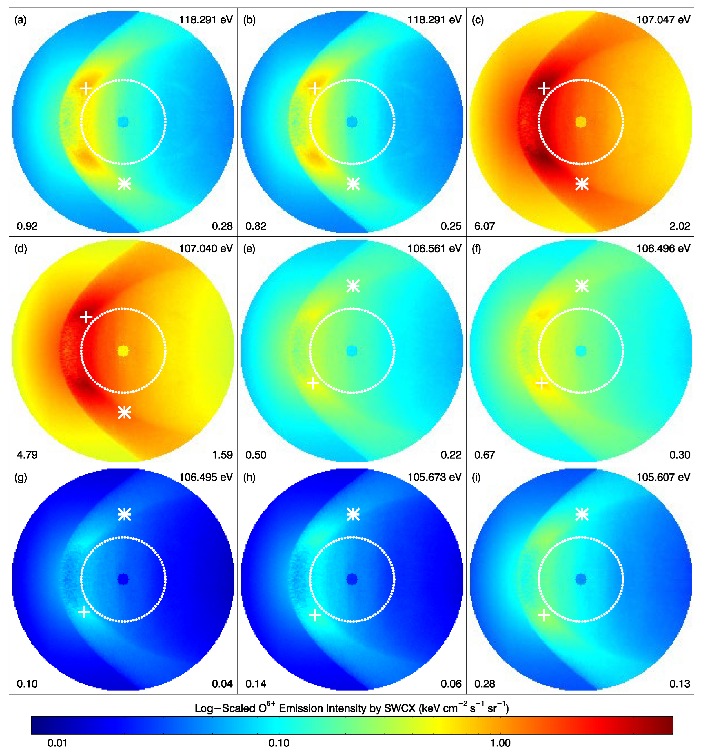
Taking Figure 3c as an example, it can be clearly seen that there is a red broadband area (magnetosheath) that is symmetrical to the XGSM axis, and its left boundary is the bow shock. The strongest emission intensity on the dayside is generated near the cusp region, and the strongest emission intensity on the nightside is located in the area near the magnetopause in the magnetosheath. The simulation results of SXR emission intensity in the magnetosheath of different O5+* ion energy states have almost the same distribution pattern. The small differences may be due to the relationship of the efficiency factor to the collision speed, as shown in Figure 2.
The strongest emission intensities for the nine spectral lines on the dayside (red) and nightside (blue) are shown in Figure 4. When the O5+* ion energy state is de-excited from 1s2 4d 2P1/2 to 1s2 2p 2D3/2, the emission intensity is the strongest, and the spectral line energy is 107.047 eV. The second-largest emission intensity is the de-excitation of O5+* ions from 1s2 4p 2P1/2 to 1s2 2p 2P3/2, with a spectral line energy of 107.040 eV. The strongest emission intensity is 6.07 keV cm−2 s−1 sr−1, and the difference between the strongest emission intensity between day and night is basically maintained at half an order of magnitude. The higher emission intensity in the dayside is primarily caused by the higher O6+ density, which directly increases the emission intensity in the dayside, while the higher relative collision velocity in the nightside results in a lower efficiency factor (Figure 2), which decreases the emission intensity.
3.3. Effects of Interplanetary Shock Waves on Soft X-ray Emission
In this section, we simulate the effect of a forward interplanetary shock passing through the Earth with a virtual camera at two special positions a and b. During this process, six stages are chosen (shown by the dashed vertical lines in Figure 5). At the first stage, the IP-TD structure has not reached the bow shock and this stage is chosen as a reference for the quiet time condition. The following stages are chosen when the IP-TD enters the magnetosheath (Stage 2), arrives at the Earth (Stage 3), and passes away from the Earth (Stages 4–6) to demonstrate the dynamic evolution of the SXR images during the passage of the IP-TD. All images are simulated at the strongest spectral line (energy 107.047 eV).
First, the initial solar wind parameters (NSW = 6 cm−3, VSW = 700 km s−1, TSW = 10 eV, BT = 8 nT, θc = 0°, and , the same as those adopted in Figure 1) were input into the hybrid model and run until an equilibrium state was achieved. Then, the solar wind IP-TD structure was inserted into the model run. The IMF was turned southward (θc = 180°) with BT increased to 16 nT, NSW was doubled to 12 cm−3, and TSW was enhanced to 15 eV. The value of in solar wind was kept at 0.001. During the following evolution of the solar wind–magnetosphere interaction, five stages after the IP-TD structure arrived at the dayside bow shock were selected to investigate the temporal variations in the X-ray emissions. It is shown that the SXR emission intensities increase significantly after the IP-TD enters the bow shock. The images also clearly show the dynamic evolution of the shock structure.
In the first stage, when the IP-TD structure does not reach the bow shock, X-ray emission intensity is low (Figure 6a,b, similar to Figure 3c). In Stage 2, when the IP-TD structure reaches about 10 RE upstream of the Earth and collides with the bow shock, the dayside maximum emission intensity occurs in the area where the IP-TD structure contacts the magnetosheath, i.e., subsolar region. As can be seen in Stages 3–6 in Figure 6, after the IP-TD structure passes through the cusp, the cusp is always the area with the highest emission intensity. An obvious signature in Figure 6 is that the X-ray emission intensity in the subsolar and low-latitude magnetosheath regions is generally lower than the intensities in the flank region or the high-latitude region, possibly because the ion velocities in the subsolar and low-latitude regions are significantly lower than those in other regions (Figure 1d,e). One can also see that a clear shock structure passed from the upstream towards the Earth (as indicated by the white arrows in Figure 6) and becomes less clear after Stage 5.
3.4. Emission Intensity Enhancement
The dayside and nightside SXR emission intensity peak values in Figure 6 are further plotted in Figure 7 to more clearly show the temporal evolutions and the difference between imaging positions. During the passing of the IP-TD structure, the emission intensity of X-rays increases with time, and the maximum value achieves 27.11 keV cm−2 s−2 sr−1 on the dayside, which is 4.5 times that before the IP-TD structure reaches the bow shock. This means that when the solar wind density increases by two times with southward IMF turning, the X-ray emission intensity can be enhanced by at least four times. Such an emission intensity enhancement is significantly smaller than the EUV emissions, which could increase 40 times [39]. The maximum emission intensity imaged at location b is always higher than that at location a, especially under conditions of enhanced solar wind conditions. The increase in the nightside is small, only about twice the initial. This may be because heavier solar wind ions (O6+) are difficult to transport to the nightside magnetosphere, while He2+ ions are lighter and can be transported to the nightside magnetosphere [39].
3.5. Bow Shock and Magnetopause Compressions
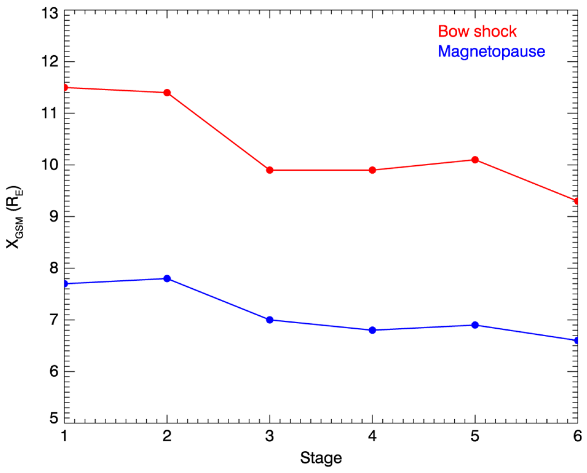
The data of the plasma temperature on the Earth’s dayside along the XGSM axis are extracted from the hybrid simulation results (Figure 8). The corresponding color of each stage is displayed in the upper right corner of the figure. In the first and second stages (green and purple lines in the figure), the temperature rises rapidly from ~1.0 eV at 11.5 RE, and quickly reaches ~1.0 keV at 10.9 RE. This sharp boundary corresponds to the bow shock. Downstream of the bow shock, there is a boundary with a sharp temperature decrease at ~8.0 RE, corresponding to the magnetopause. Therefore, the positions where the temperature dramatically increases and decreases are identified as the positions of bow shock and magnetopause, respectively.
From Stage 3 on, when the IP-TD structure enters the magnetosheath, both the bow shock and the magnetopause are significantly compressed and move towards the Earth. We extract the position data of the bow shock and magnetopause in the six stages in Figure 8 and draw a line chart of the position changes in Figure 9. It can be clearly seen that the bow shock moves from 11.4 RE to 9.3 RE, and the magnetopause moves from 7.8 RE to 6.6 RE. This is a very strong compression of the magnetosphere. The compression is the most significant during the period when the IP-TD contacts the dayside bow shock and passes through the dayside magnetopause (Stage 2 to Stage 3).
Figure 10 shows the simulated SXR emission profiles along the XGSM axis from position a. The vertical solid and dashed lines show the positions of bow shock and magnetopause in Figure 8, respectively. It is shown that the position of the bow shock corresponds well with the right edge of the radial profile of SXR emission, that is, the position of the bow shock is consistent with the coordinates of the first sudden increase in SXR emission. Therefore, the SXR emission can be reliably utilized to identify the location and shape of the bow shock in future X-ray imaging. However, the magnetopause structure in SXR images may not be so clear due to the LOS overlapping effect. Other methods should be investigated in the future to extract the magnetopause structures in X-ray images. In the future, more systematic simulations should be conducted to elucidate the X-ray emission characteristics under different solar wind and IMF conditions, so as to find ways to extract the position of the magnetopause. Fortunately, the soft X-ray imager onboard the SMILE satellite will capture real X-ray images of the magnetosheath in the near future. A comparison between the X-ray images and the in situ magnetopause crossing data will help us figure out the signature of magnetopause in the X-ray images. We hope to further establish an accurate extraction algorithm for the magnetopause.
4. Conclusions
This paper uses the global hybrid simulation model, the geocoronal hydrogen model, and the SASAL to simulate the spectral lines of solar wind O6+ ions to study the impact of interplanetary shock on SXR emission in the Earth’s magnetosheath. The main results are summarized as follows:
- A global hybrid model is used to simulate the number density, velocity, and temperature distribution of O6+ in the magnetosheath. Then, the SASAL is used to calculate the state distributions of excited O5+* ions, which are generated from the collisions between O6+ ions and hydrogen atoms, to obtain the efficiency factors for the X-ray emissions. Then, the X-ray emission intensities are simulated at 60.0 RE at the dusk side and at the north pole.
- It is found that there are two closed strong emission lines for O5+* at 10.582 nm and 10.583 nm, corresponding to energies of 107.047 eV and 107.040 eV. The efficiency factors of both lines vary significantly with collision speed. All energy states of O5+* ions have almost the same distribution pattern in the simulated images. The strongest emission intensity on the dayside is generated in the cusp region, and the strongest emission intensity on the nightside is in the area near the magnetopause in the magnetosheath. This is because the O6+ density is the highest while the velocity is the lowest in the cusp region where the magnetic field is converging, providing favorable conditions for generating strong emissions.
- During the passage of an IP-TD structure, significant emission intensity enhancement and compressions of both bow shock and magnetopause are observed in the simulations. The passage of the shock in the magnetosheath is clearly shown in the simulated images. The emission intensities simulated at dusk are always stronger than those simulated at the north pole, possibly because the solar wind heavy ions in the magnetosheath are mainly confined to near the equatorial region.
- The emission intensity profiles can be reliably used to extract the location of the bow shock, while the location of the magnetopause is difficult to identify, possibly due to the LOS overlapping effect.
During the passing of solar wind structures (such as CME, discontinuity, IP shock, etc.) in the magnetosphere, the influence in the magnetosheath can be clearly observed in the X-ray images, such as the earthward motions of bow shock and magnetopause. Thus, imagers with large fields of view (e.g., the SMILE SXI and other EUV imagers in the future) will be powerful in monitoring the large-scale dynamic evolution of the magnetosheath and revealing the mass and energy transportation from solar wind into the magnetosphere. If the imagers are capable of distinguishing X-ray spectral lines, the dynamics of specific heavy ions in the magnetosheath can be traced. The emission properties of other solar wind heavy ions will be investigated in the future.
Author Contributions
Conceptualization, F.H.; methodology, F.H., Z.Z., G.L. and X.W.; software, F.H., Z.Z., G.L. and X.W.; validation, F.H., X.-X.Z. and X.W.; formal analysis, Z.Z.; investigation, Z.Z. and F.H.; writing—original draft preparation, Z.Z.; writing—review and editing, F.H., X.-X.Z., G.L., X.W. and Y.W.; visualization, Z.Z.; supervision, F.H.; project administration, F.H.; funding acquisition, F.H. All authors have read and agreed to the published version of the manuscript.
Funding
This research was funded by the National Key R&D Program of China (2021YFA0718600) and the National Natural Science Foundation of China (42222408, 41931073). F.H. was supported by the Youth Innovation Promotion Association of the Chinese Academy of Sciences (Y2021027).
Data Availability Statement
The data presented in the article are available upon request from the author at the following email address: [email protected].
Acknowledgments
We appreciate the reviewers for their valuable comments and suggestions.
Conflicts of Interest
The authors declare no conflicts of interest.
References
- Sonett, C.P.; Abrams, I.J. The distant geomagnetic field: 3. Disorder and shocks in the magnetopause. J. Geophys. Res. 1963, 68, 1233–1263. [Google Scholar] [CrossRef]
- Nabert, C.; Glassmeier, K.H.; Plaschke, F. A new method for solving the MHD equations in the magnetosheath. In Annales Geophysicae; Copernicus Publications: Göttingen, Germany, 2013; Volume 31, No. 3; pp. 419–437. [Google Scholar]
- Dimmock, A.P.; Nykyri, K. The statistical mapping of magnetosheath plasma properties based on THEMIS measurements in the magnetosheath interplanetary medium reference frame. J. Geophys. Res. Space Phys. 2013, 118, 4963–4976. [Google Scholar] [CrossRef]
- Omidi, N.; Zhang, H.; Chu, C.; Turner, D. Parametric dependencies of spontaneous hot flow anomalies. J. Geophys. Res. Space Phys. 2014, 119, 9823–9833. [Google Scholar] [CrossRef]
- Breuillard, H.; Le Contel, O.; Chust, T.; Berthomier, M.; Retino, A.; Turner, D.L.; Nakamura, R.; Baumjohann, W.; Cozzani, G.; Catapano, F.; et al. The properties of Lion roars and electron dynamics in mirror mode waves observed by the Magnetospheric MultiScale Mission. J. Geophys. Res. Space Phys. 2018, 123, 93–103. [Google Scholar] [CrossRef]
- Zhao, J.; Wang, T.; Shi, C.; Graham, D.B.; Dunlop, M.W.; He, J.; Tsurutani, B.T.; Wu, D. Ion and electron dynamics in the presence of mirror, electromagnetic ion cyclotron, and whistler waves. Astrophys. J. 2019, 883, 185. [Google Scholar] [CrossRef]
- Zhong, Y.; Wang, H.; Zhang, K.; Xia, H.; Qian, C. Local time response of auroral electrojet during magnetically disturbed periods: DMSP and CHAMP coordinated observations. J. Geophys. Res. Space Phys. 2022, 127, e2022JA030624. [Google Scholar] [CrossRef]
- Cravens, T.E. Comet Hyakutake X-ray source: Charge transfer of solar wind heavy ions. Geophys. Res. Lett. 1997, 24, 105–108. [Google Scholar] [CrossRef]
- Paresce, F.; Fahr, H.; Lay, G. A search for interplanetary He II, 304-A emission. J. Geophys. Res. Space Phys. 1981, 86, 10038–10048. [Google Scholar] [CrossRef]
- Lisse, C.M.; Christian, D.J.; Dennerl, K.; Meech, K.J.; Petre, R.; Weaver, H.A.; Wolr, S.J. Charge exchange-induced X-ray emission from Comet C/1999 S4 (LINEAR). Science 2001, 292, 1343–1348. [Google Scholar] [CrossRef]
- Ringuette, R.; Koutroumpa, D.; Kuntz, K.D.; Kaaret, P.; Jahoda, K.; LaRocca, D.; Kounkel, M.; Richardson, J.; Zajczyk, A.; Bluem, J. HaloSat observations of heliospheric solar wind charge exchange. Astrophys. J. 2021, 918, 41. [Google Scholar] [CrossRef]
- Zhou, Y.; Yamasaki, N.Y.; Toriumi, S.; Mitsuda, K. Geocoronal Solar Wind Charge Exchange Process Associated with the 2006-December-13 Coronal Mass Ejection Event. J. Geophys. Res. Space Phys. 2023, 128, e2023JA032069. [Google Scholar] [CrossRef]
- Ishikawa, K.; Ezoe, Y.; Miyoshi, Y.; Terada, N.; Mitsuda, K.; Ohashi, T. Suzaku observation of strong solar-wind charge-exchange emission from the terrestrial exosphere during a geomagnetic storm. Publ. Astron. Soc. Jpn. 2013, 65, 63. [Google Scholar] [CrossRef]
- Ringuette, R.; Kuntz, K.D.; Koutroumpa, D.; Kaaret, P.; LaRocca, D.; Richardson, J. Observations of Magnetospheric Solar Wind Charge Exchange. Astrophys. J. 2023, 955, 139. [Google Scholar] [CrossRef]
- Zhang, Y.J.; Sun, T.R.; Carter, J.A.; Liu, W.H.; Sembay, S.; Zhang, S.N.; Ji, L.; Wang, C. Two methods for separating the magnetospheric solar wind charge exchange soft X-ray emission from the diffuse X-ray background. Earth Planet. Phys. 2023, 8, 119–132. [Google Scholar] [CrossRef]
- Connor, H.K.; Sibeck, D.G.; Collier, M.R.; Baliukin, I.I.; Branduardi-Raymont, G.; Brandt, P.C.; Buzulukova, N.Y.; Collado-Vega, Y.M.; Escoubet, C.P.; Fok, M.-C.; et al. Soft X-ray and ENA Imaging of the Earth’s Dayside Magnetosphere. J. Geophys. Res. Space Phys. 2021, 126, e2020JA028816. [Google Scholar] [CrossRef] [PubMed]
- Sun, T.R.; Wang, C.; Sembay, S.F.; Lopez, R.E.; Escoubet, C.P.; Branduardi-Raymont, G.; Zheng, J.H.; Yu, X.Z.; Guo, X.C.; Dai, L.; et al. Soft X-ray imaging of the magnetosheath and cusps under different solar wind conditions: MHD simulations. J. Geophys. Res. Space 2019, 124, 2435–2450. [Google Scholar] [CrossRef]
- Raab, W.; Branduardi-Raymont, G.; Wang, C.; Dai, L.; Donovan, E.; Enno, G.; Escoubet, P.; Holland, A.; Li, J.; Kataria, D.; et al. SMILE: A joint ESA/CAS mission to investigate the interaction between the solar wind and Earth’s magnetosphere. Proc. SPIE 2016, 9905, 990502-1–990502-9. [Google Scholar] [CrossRef]
- Collier, M.R.; Porter, F.S.; Sibeck, D.G.; Carter, J.A.; Chiao, M.P.; Chornay, D.J.; Cravens, T.; Galeazzi, M.; Keller, J.W.; Koutroumpa, D.; et al. Prototyping a global soft X-ray imaging instrument for heliophysics, planetary science, and astrophysics science. Astron. Nachr. 2012, 333, 378–382. [Google Scholar] [CrossRef]
- Somana, M.R.; Halla, D.J.; Hollanda, A.D.; Burgona, R.; Buggeya, T.; Skottfelta, J.; Sembayb, S.; Drummb, P.; Thornhillb, J.; Readb, A.; et al. The SMILE Soft X-ray Imager (SXI) CCD design and development. J. Instrum. 2018, 13, C01022. [Google Scholar] [CrossRef]
- Schwadron, N.A.; Cravens, T.E. Implications of solar wind composition for cometary X-rays. Astrophys. J. 2000, 544, 558. [Google Scholar] [CrossRef]
- Robertson, I.P.; Collier, M.R.; Cravens, T.E.; Fok, M.-C. X-ray emission from the terrestrial magnetosheath including the cusps. J. Geophys. Res. Space Phys. 2006, 111, A12105. [Google Scholar] [CrossRef]
- Lin, Y.; Wang, X.Y.; Lu, S.; Perez, J.D.; Lu, Q. Investigation of storm time magnetotail and ion injection using three-dimensional global hybrid simulation. J. Geophys. Res. Space Phys. 2014, 119, 7413–7432. [Google Scholar] [CrossRef]
- Lin, Y.; Wang, X.Y. Three-dimensional global hybrid simulation of dayside dynamics associated with the quasi-parallel bow shock. J. Geophys. Res. Space Phys. 2005, 110, A12216. [Google Scholar] [CrossRef]
- Swift, D.W. Use of a hybrid code for global-scale plasma simulation. J. Comput. Phys. 1996, 126, 109–121. [Google Scholar] [CrossRef]
- Kivelson, M.G.; Russell, C.T. (Eds.) Introduction to Space Physics; Cambridge University Press: Cambridge, UK, 1995; p. 31. [Google Scholar]
- Lepri, S.T.; Landi, E.; Zurbuchen, T.H. Solar wind heavy ions over solar cycle 23: ACE/SWICS measurements. Astrophys. J. 2013, 768, 94. [Google Scholar] [CrossRef]
- Von Steiger, R.; Zurbuchen, T.H.; McComas, D.J. Oxygen flux in the solar wind: Ulysses observations. Geophys. Res. Lett. 2010, 37, L22101. [Google Scholar] [CrossRef]
- Hodges, R.R., Jr. Monte Carlo simulation of the terrestrial hydrogen exosphere. J. Geophys. Res. Space Phys. 1994, 99, 23229–23247. [Google Scholar] [CrossRef]
- Brinkmann, R.T. Departures from Jeans’ escape rate for H and He in the Earth’s atmosphere. Planet. Space Sci. 1970, 18, 449–478. [Google Scholar] [CrossRef]
- Cole, K.D. Theory of some Quiet Magnetospheric [Phenomena related to the Geomagnetic Tail. Nature 1966, 211, 1385–1387. [Google Scholar] [CrossRef]
- Hodges, R.R., Jr.; Tinsley, B.A. Charge exchange in the Venus ionosphere as the source of the hot exospheric hydrogen. J. Geophys. Res. Space Phys. 1981, 86, 7649–7656. [Google Scholar] [CrossRef]
- Liang, G.Y.; Li, F.; Wang, F.L.; Wu, Y.; Zhong, J.Y.; Zhao, G. X-ray and EUV spectroscopy of various astrophysical and laboratory plasmas: Collisional, photoionization and charge-exchange plasmas. Astrophys. J. 2014, 783, 124. [Google Scholar] [CrossRef]
- Verner, D.A.; Ferland, G.J.; Korista, K.T.; Yakovlev, D.G. Atomic data for astrophysics. II. New analytic fits for photoionization cross sections of atoms and ions. Astrophys. J. 1996, 465, 487. [Google Scholar] [CrossRef]
- Salop, A.; Olson, R.E. Charge exchange between H(1s) and fully stripped heavy ions at low-keV impact energies. Phys. Rev. A 1976, 13, 1312–1320. [Google Scholar] [CrossRef]
- Liang, G.Y.; Zhu, X.L.; Wei, H.G.; Yuan, D.W.; Zhong, J.Y.; Wu, Y.; Hutton, R.; Cui, W.; Cui, X.W.; Zhao, G. Charge-exchange soft X-ray emission of highly charged ions with inclusion of multiple-electron capture. Mon. Not. R. Astron. Soc. 2021, 508, 2194–2203. [Google Scholar] [CrossRef]
- Liang, G.Y.; Sun, T.R.; Lu, H.Y.; Zhu, X.L.; Wu, Y.; Li, S.B.; Wei, H.G.; Yuan, D.W.; Zhong, J.Y.; Cui, W.; et al. X-ray morphology due to charge-exchange emissions used to study the global structure around Mars. Astrophys. J. 2023, 943, 85. [Google Scholar] [CrossRef]
- Kharchenko, V.; Dalgarno, A. Spectra of cometary X rays induced by solar wind ions. J. Geophys. Res. Space Phys. 2000, 105, 18351–18359. [Google Scholar] [CrossRef]
- He, F.; Zhang, X.X.; Wang, X.Y.; Chen, B. EUV emissions from solar wind charge exchange in the Earth’s magnetosheath: Three-dimensional global hybrid simulation. J. Geophys. Res. Space Phys. 2015, 120, 138–156. [Google Scholar] [CrossRef]
Figure 1.
Plasma parameter profile. (a–c) The O6+ ion number density in xy, xz, and yz planes in the GSM coordinate system, respectively. (d–f) The solar wind speed VSW in xy, xz, and yz planes in the GSM coordinate system, respectively. (g–i) The solar wind temperature TSW in xy, xz, and yz planes in the GSM coordinate system, respectively. (j–l) The hydrogen atom number density nH in xy, xz, and yz planes in the GSM coordinate system, respectively. The color bars are shown on the right. The SW-IMF parameters are NSW = 6 cm−3, VSW = 700 km s−1, TSW = 10 eV, BT = 8 nT, θc = 0°, and = 0.001.

Figure 2.
Changes in different SXR α parameters with collision speed. The colors of different energies are shown in the upper right corner.
Figure 2.
Changes in different SXR α parameters with collision speed. The colors of different energies are shown in the upper right corner.

Figure 3.
Intensity distribution for all spectral lines of O6+ integrated along the line of sight at position b. (a–i) Intensity distributions for the nine spectral lines listed in Table 1. The energy of the spectral line, the peak intensity on the dayside (indicated by crosses), and the peak intensity on the nightside (indicated by asterisks) are shown in the upper right corners, lower left corners, and lower right corners of each panel. The conical angle of the field of the virtual camera is 40°, and the dotted circles indicate a 15° field of view. The image is projected in the GSM xz plane, with the +XGSM axis pointing left and the +ZGSM axis pointing up. The logarithmically scaled color bar is located at the bottom.

Figure 4.
The strongest day and night emission intensities of SXR with different energies.

Figure 5.
The IP-TD structure in the solar wind is added to the simulation. The time nodes of the six stages of simulation are represented by vertical dashed lines in the figure.
Figure 5.
The IP-TD structure in the solar wind is added to the simulation. The time nodes of the six stages of simulation are represented by vertical dashed lines in the figure.

Figure 6.
Magnetosheath X-ray emission intensity simulated at the two locations in a (0.0, 0.0, 60.0 RE) and b (0.0, 60.0 RE, 0.0) at six stages (Stage 1–6) during the passing of the IP-TD in Figure 5. (a,b) Stage 1 at both locations. (c,d) Stage 2 at both locations. (e,f) Stage 3 at both locations. (g,h) Stage 4 at both locations. (i,j) Stage 5 at both locations. (k,l) Stage 6 at both locations.The column labeled with ‘Location a’ shows the images in the GSM xy plane and the column labeled with ‘Location b’ shows the images in the GSM xz plane. The Sun is always located on the left. The white arrows indicate the shock structure of the IP-TD. The white crosses and asterisks in each panel indicate the locations of peak intensity in dayside and nightside, respectively.

Figure 7.
Magnetosheath SXR emission intensity peaks at different stages during the IP-TD passage.

Figure 8.
Plasma temperature along the XGSM axis at six stages. The solid and dashed lines represent the positions of the bow shock and the magnetopause in the six stages, respectively. The corresponding color for each stage is shown in the upper right corner.
Figure 8.
Plasma temperature along the XGSM axis at six stages. The solid and dashed lines represent the positions of the bow shock and the magnetopause in the six stages, respectively. The corresponding color for each stage is shown in the upper right corner.

Figure 9.
Bow shock and magnetopause position diagram at different stages.

Figure 10.
Changes in SXR emission intensity of perspective + XGSM axis at position a at different stages. The solid and dashed lines represent the positions of the bow shock and the magnetopause in the six stages, respectively.
Figure 10.
Changes in SXR emission intensity of perspective + XGSM axis at position a at different stages. The solid and dashed lines represent the positions of the bow shock and the magnetopause in the six stages, respectively.


Table 1.
O5+* ion energy state changes correspond to SXR wavelength and energy.
| Number | Energy State | Wavelength (nm) | Energy (eV) |
|---|---|---|---|
| 1 | 1s2 5d 2P1/2 → 1s2 2p 2D3/2 | 10.481 | 118.291 |
| 2 | 1s2 5p 2P1/2 → 1s2 2p 2P3/2 | 10.481 | 118.291 |
| 3 | 1s2 4d 2P1/2 → 1s2 2p 2D3/2 | 11.582 | 107.047 |
| 4 | 1s2 4p 2P1/2 → 1s2 2p 2P3/2 | 11.583 | 107.040 |
| 5 | 1s2 5d 2P3/2 → 1s2 2p 2D5/2 | 11.635 | 106.561 |
| 6 | 1s2 5f 2P1/2 → 1s2 3s 2F5/2 | 11.642 | 106.496 |
| 7 | 1s2 5d 2P1/2 → 1s2 3s 2D5/2 | 11.642 | 106.495 |
| 8 | 1s2 5p 2P3/2 → 1s2 2p 2P1/2 | 11.732 | 105.673 |
| 9 | 1s2 5p 2P1/2 → 1s2 3s 2P1/2 | 11.740 | 105.607 |
Disclaimer/Publisher’s Note: The statements, opinions and data contained in all publications are solely those of the individual author(s) and contributor(s) and not of MDPI and/or the editor(s). MDPI and/or the editor(s) disclaim responsibility for any injury to people or property resulting from any ideas, methods, instructions or products referred to in the content. |
© 2024 by the authors. Licensee MDPI, Basel, Switzerland. This article is an open access article distributed under the terms and conditions of the Creative Commons Attribution (CC BY) license (https://creativecommons.org/licenses/by/4.0/).
Share and Cite
MDPI and ACS Style
Zhang, Z.; He, F.; Zhang, X.-X.; Liang, G.; Wang, X.; Wei, Y. Solar Wind Charge-Exchange X-ray Emissions from the O5+ Ions in the Earth’s Magnetosheath. Remote Sens. 2024, 16, 1480. https://doi.org/10.3390/rs16091480
AMA Style
Zhang Z, He F, Zhang X-X, Liang G, Wang X, Wei Y. Solar Wind Charge-Exchange X-ray Emissions from the O5+ Ions in the Earth’s Magnetosheath. Remote Sensing. 2024; 16(9):1480. https://doi.org/10.3390/rs16091480
Chicago/Turabian StyleZhang, Zhicheng, Fei He, Xiao-Xin Zhang, Guiyun Liang, Xueyi Wang, and Yong Wei. 2024. "Solar Wind Charge-Exchange X-ray Emissions from the O5+ Ions in the Earth’s Magnetosheath" Remote Sensing 16, no. 9: 1480. https://doi.org/10.3390/rs16091480
Note that from the first issue of 2016, this journal uses article numbers instead of page numbers. See further details here.