Satellite-Derived Variability of Sea Surface Salinity and Geostrophic Currents off Western Patagonia

Abstract

The coastal ocean off western Patagonia is one of the main coastal regions with high freshwater inputs from rivers, rain, and glaciers in the Southern Hemisphere. This study conducts an analysis of the seasonal and interannual variations in sea surface salinity and meridional geostrophic transports, specifically focusing on the Cape Horn Current, using improved satellite-derived data of sea surface salinity (SSS) and geostrophic velocities spanning an ∼11-year period (September 2011–August 2022). Our results reveal a clear salinity minimum in a coastal band between 42–54°S associated with the highest freshwater content. The average geostrophic currents are stronger south of 49°S, in line with the location of the Cape Horn Current. The average salinity minimum tends to disappear south of 54°S, with salinity values increasing slightly southward. The seasonal cycle of salinity shows the most pronounced minimum in summer (∼33.2–33.4). The greatest variability in salinity (standard deviation of salinity fields) occurs in the southern region of the Cape Horn Current. Hovmöller plots reveal two cores of minimum salinity observed in spring and summer (∼33.3–33.4). The freshwater off the Gulf of Penas contributes to the northern core. The meridional geostrophic transport differs between the northern and southern sections, with transports predominantly towards the Equator (Pole) north (south) of about 47–48°S during spring–summer. There is a marked seasonal variability in the magnitude and northern limit of the southward-flowing Cape Horn Current, being extended further north during winter and with a maximum average magnitude during summer–fall (about $-2\times {10}^4$ m² s⁻¹). On the interannual scale, a major drop in surface salinity occurred off northern and central Patagonia during 2018–2019. Finally, a potential long-term freshening trend is observed in the coastal area off southern Patagonia (south of 52°S), although prolonged data records are essential to confirm this pattern.

1. Introduction

At high latitudes, salinity has a significant impact on density fields; it also influences ocean currents and mixing [1]. In general, studies of freshwater outflows and plumes (and low-salinity waters) in the coastal ocean have mainly been focused on localized sources from rivers along mid-latitudes (e.g., [2,3,4,5]). Nonetheless, the largest contributions of freshwater into the coastal ocean occur in subpolar/polar regions as a response to increased precipitation, river discharges, and ice melting (e.g., [6,7,8,9]). As a result, low-density, buoyancy-driven coastal currents develop in these high-latitude systems, including the Greenland Current [10], Norwegian Current [11], Alaska Current [12], and the Cape Horn Current [13]. The later is less studied, mainly because of the lack of long-term in situ observations [14].

The start of satellite-derived sea surface salinity measurements with the Soil Moisture and Ocean Salinity (SMOS) missions opened a new era in the study of freshwater systems at regional to large spatial scales. Subsequently, measurements from the Aquarius mission [15] and the Soil Moisture Active Passive (SMAP) mission opened a new era in the study of freshwater systems at regional to large spatial scales (e.g., [1,9,16]). Based on these three missions, NASA has created the Multi-Mission Optimally Interpolated Sea Surface Salinity (OISSS) product with a 0.25-degree spatial resolution [17]. It generally matches well with the data from the In Situ Analysis System (ISAS), which is primarily based on interpolation using measurements from Argo floats and other in situ measurements [18]. Additionally, the global-scale salinity patterns observed in OISSS show only minor differences compared to the Simple Ocean Data Assimilation (SODA 3.11.2) and GLORYS12V1 ocean datasets reanalysis [19]. These datasets show that the South Pacific exhibits the lowest salinities in the polar zone and along the coasts of central and southern Chile, coinciding with a relative minimum in salinity off Patagonia [19,20]. It has been observed that regions such as the coastal ocean off Patagonia do not experience such extreme environmental conditions as the southern polar regions [20]. Therefore, the OISSS product should accurately represent the spatio-temporal variability of surface salinity on a regional scale.

Studies of the low-salinity freshwater conditions off western Patagonia have been limited. An extensive low-salinity tongue extending from approximately 40ºS to 56ºS, with the freshwater band extending up to 5º offshore, has principally been documented [8,21]. An extended analysis showed the contrasting seasonal variability and vertical structure of the freshwater wedge along the meridional gradient off western Patagonia [9], whereas the dominant biogeochemical conditions were described along the freshwater gradient off central Patagonia by Galán et al. [22]. To the best of our knowledge, this is the first study analyzing the spatio-temporal variability of the low-salinity waters off western Patagonia based on the improved OISSS product, whereas the transport of the Cape Horn Current has been recently inspected based on sea level variability [14]. Section 2 describes the data and methods with emphasis on the satellite sea surface salinity measurements and the geostrophic velocities. Finally, Section 3 presents the main results and discussion on the spatio-temporal variability of low-salinity waters and geostrophic currents along the coastal ocean off western Patagonia.

2. Materials and Methods

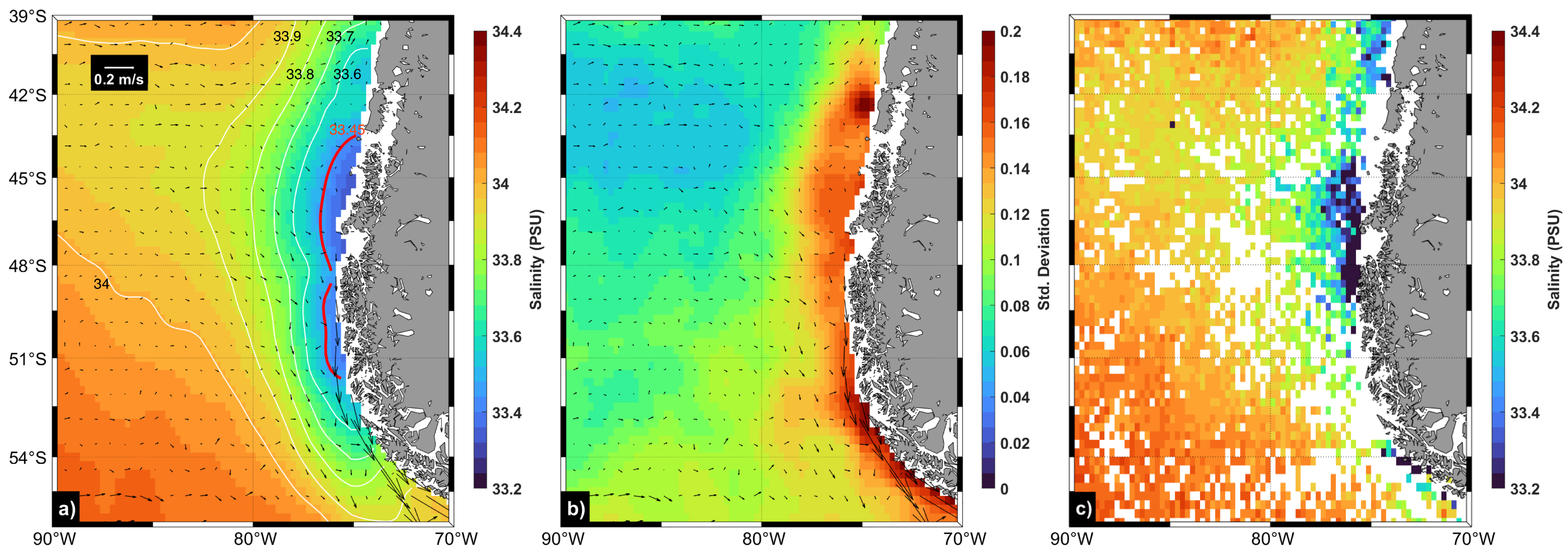
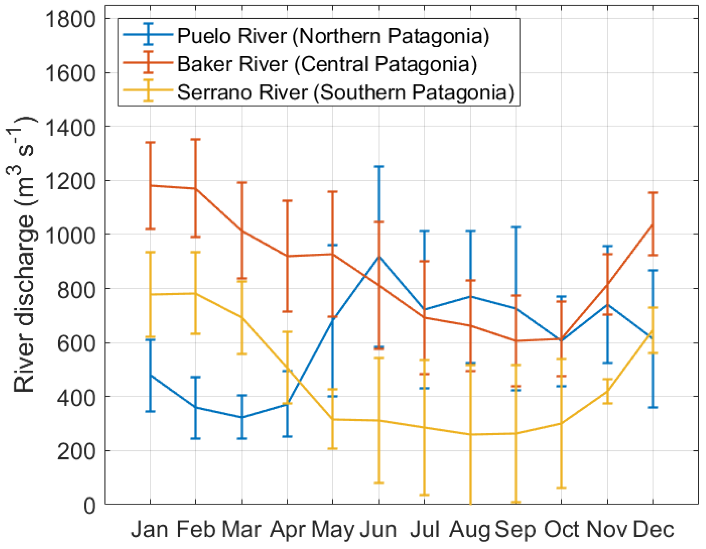
2.1. Datasets

Satellite data have allowed the study of sea surface salinity and freshwater conditions worldwide at multiple spatio-temporal scales (e.g., [23,24,25,26]). Here, we used the Multi-Mission Optimally Interpolated Sea Surface Salinity (OISSS) Level 4 V1.0 dataset [27], accessed through https://podaac.jpl.nasa.gov/dataset/OISSS_L4_multimission_7day_v1 (accessed on 20 November 2023). OISSS is an L4 product generated by merging the L2 data of the AQUARIUS, SMOS, and SMAP datasets using optimal interpolation to generate global maps of sea surface salinity with a 4-day temporal resolution and 0.25° × 0.25° spatial resolution. The product uses SMOS data to achieve temporal continuity along the period and is validated using data from ARGO buoys and moored buoys. This dataset has been used for different regional studies (e.g., [28,29,30,31]) and studies at the global scale (e.g., [32,33]). This is the first time that it has been used for a detailed study off of Chilean Patagonia. Monthly averages and anomalies of SSS were computed using the OISSS product at each pixel from September of 2011 to August 2022. Anomalies were calculated by subtracting the corresponding monthly climatology from each monthly average within the study domain (39–56°S and 70°W and 90°W).

Geostrophic currents were obtained from the SSALTO/DUACS Delayed-Time Level-4 product distributed by AVISO (https://www.aviso.altimetry.fr/en/data/products/sea-surface-height-products/global/gridded-sea-level-heights-and-derived-variables.html (accessed on 27 November 2023). These currents were derived from daily sea level height anomaly values with a spatial resolution of 0.25° × 0.25° spanning the period from 2011 to 2022, which aligns with the data available in the OISSS dataset. Monthly values were determined for each pixel.

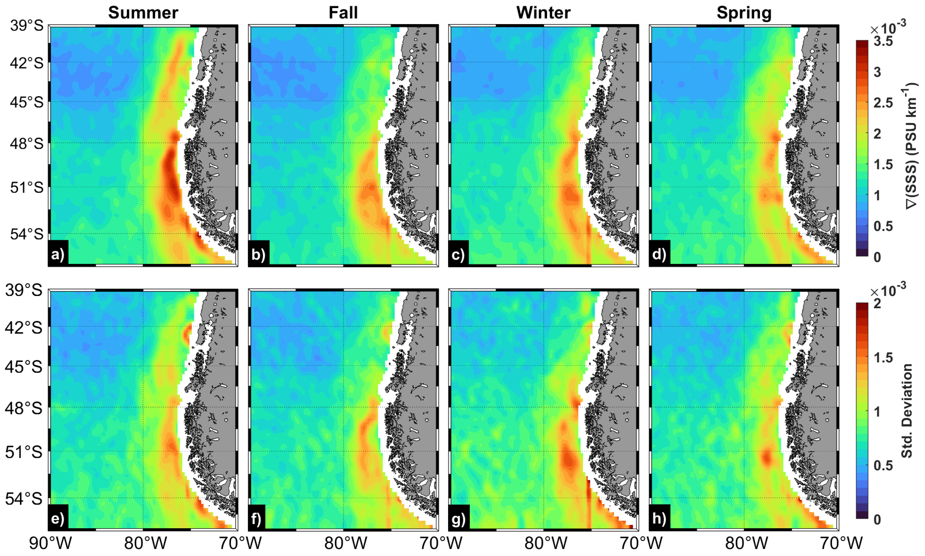
2.2. Salinity Gradients

Regions of salinity gradients/fronts were characterized by calculating the gradient magnitude using the central difference method as in previous studies of SST fronts [34,35,36]:

$${\nabla }_{x}SSS(i,j)=(SS{S}_{(i+1,j)}-SS{S}_{(i-1,j)})/(X_{(i+1,j)}-X_{(i-1,j)})$$

(1)

$${\nabla }_{y}SSS(i,j)=(SS{S}_{(i,j+1)}-SS{S}_{(i,j-1)})/(Y_{(i,j+1)}-Y_{(i,j-1)})$$

(2)

$$|\nabla SSS|(i,j)={\{{\left({\nabla }_{x}SS{S}_{(i,j)}\right)}^2+{\left({\nabla }_{y}SS{S}_{(i,j)}\right)}^2\}}^{1/2}$$

(3)

where SSS is the sea surface salinity from OISSS, and X and Y are the zonal and meridional axes. The index i and j stands for the positions along the zonal and meridional direction, respectively.

2.3. Meridional Transports

For a detailed analysis of the nearshore variability in SSS and meridional transports, a coastal band of 100 km was averaged at each time step considering the last available pixel in the SSS data. Coastal monthly SSS was computed at each latitude by averaging the pixels inside the coastal band. In the same way, meridional transports ($V_{transport}$) were computed in this 100 km band by integrating the meridional geostrophic velocities at each latitude:

$$V_{transport}(y,t)={\int }_{x_0\left(y\right)}^{x_0\left(y\right)-100 \mathrm{k}\mathrm{m}}{V}_{geo}(x,y,t)dx$$

(4)

where $x_0$ is the last pixel with data near the coast, and $V_{geo}$ is the meridional velocity at each grid point.

2.4. EOF Analysis

In order to determine the leading patterns of SSS anomalies in the study area, an empirical orthogonal functions (EOF) analysis was performed using the monthly SSS anomalies. A single value decomposition (SVD) approach was used to compute the EOFs considering the number of pixels and was much greater than the number of time steps [37].

3. Results and Discussion

3.1. Seasonal Variability of Sea Surface Salinity off Western Patagonia

The mean SSS off western Patagonia shows minimum values in a coastal band mostly restricted to the east of 80°W and the meridional extent between the latitudes 54–42°S (Figure 1a). On the other hand, the average maximum salinities are found around the southwest area of the domain, which produces an SSS gradient towards the northeast, reaching the aforementioned salinity minimum. This is consistent with the average surface (0–10 m) salinity from the Argo profiling floats in the study area (Figure 1c). The area of the salinity minimum represents the zone with the highest freshwater content observed in the region, coinciding with the greatest seasonal variability in SSS (Figure 1b). This occurs because of the considerable temporal variability in freshwater discharges into the coastal region. This freshwater pattern coincides with the contribution from rivers and glacial melting in the fjords and channels of Chilean Patagonia (e.g., [9,38]). In addition, the most intense average geostrophic currents occur south of 49°S (Figure 1), increasing in magnitude towards the south, which is consistent with the location of the Cape Horn Current [14,39]. It is noteworthy that the salinity minimum tends to disappear south of 54°S, with salinity values increasing slightly southward (Figure 1a). This is in agreement with the meridional analysis of Saldías et al. [9], in which the stratification was mostly controlled by the cold temperatures off southern Patagonia, and the freshwater content was mostly confined to the coastal ocean off central Patagonia. Another potential explanation for the enhanced southward salinity could be the influence of surface winds. Pérez-Santos et al. [40] identified a more pronounced positive (upwelling) Ekman vertical velocity south of 50°S, facilitating the mixing of saline water from the subsurface layer. Furthermore, Yu [41] highlighted the importance of anomalous vertical entrainment in shaping the sea surface salinity (SSS) characteristics off western Patagonia.

The SSS off western Patagonia has a seasonal cycle marked by the most pronounced saline minimum occurring in summer (Figure 2a). During this season, a contrast in the salinity minimum is evident within the coastal band, as a core with even lower salinities emerges between about 43 and 48°S. There is a lower presence of freshwater in spring compared to summer (Figure 2d), although these two seasons are the ones that exhibit the greatest amount of freshwater in this coastal ocean (e.g., [9]). In spring, the salinity minimum presents a similar spatial distribution (Figure 2d). The lowest salinity is restricted to the coastal area south of 48°S in fall and centered around 51°S (Figure 2b). As mentioned above, the Cape Horn Current is evidenced in the average geostrophic velocities and seems to be fairly persistent throughout the annual cycle (Figure 2). On the other hand, the SSS exhibits its greatest variability (standard deviation) in the coastal band (Figure 2e–h). Notice that the highest salinity variability, except for the area off Chiloé Island around 42°S, occurs primarily in the southern region of the Cape Horn Current (Figure 2e–h). The surface salinity exhibits its greatest variability during the summer season (Figure 2e). It is not clear in which season the lowest variability in salinity occurs; fall, winter, and spring show similar magnitudes of variability (Figure 2f–h), though with differences in the spatial patterns. An analysis of the seasonal variability of surface salinity from the Argo floats reveals differences compared to the seasonal climatology of sea surface salinity (SSS) from OISSS for the same study period (Figure 2i–l vs. Figure 2a–d). The average grid cells from the Argo floats exhibit fresher conditions. These discrepancies result from relatively sparse data points in the Argo float averages compared to satellite SSS images. In fact, a significant portion of the area covered lacks Argo floats in the analysis (white areas in Figure 2i–l).

To clarify the seasonal variability of river discharges and SSS and geostrophic velocities in the coastal band where freshwater dominates, the seasonal cycles of large rivers and Hovmöller plots (considering a coastal band extending 100 km offshore) are presented in Figure 3 and Figure 4, respectively. Rivers of northern Patagonia, such as the Puelo River, present a seasonal cycle with the largest discharges in winter and spring, whereas large rivers in central and southern Patagonia (e.g., Baker and Serrano) present maximum discharges in spring and summer (Figure 3). Coherently, the average fresher signature off central Patagonia starts in spring (August–October) in the area between 45°S and 48°S. Two cores of minimum salinities continue in summer (from January to March) and are centered around 43–48°S and 49–52°S (Figure 4a). The presence of the northern core may be attributed to the contribution of freshwater from the Gulf of Penas (e.g., [22]), which accounts for the freshwater discharges from the Pascua and Baker rivers (e.g., [42,43]). This input of freshwater is highly significant in the region as it alters the physical and biogeochemical characteristics of the upper ocean [9,22]. In terms of water masses, sub-Antarctic water (SAAW), Equatorial subsurface water (ESSW), Antarctic intermediate water (AAIW), and Pacific deep water (PDW) have been identified in previous studies in the same area [44,45,46,47]. The SAAW occupies a surface layer of about 100 m, whereas ESSW penetrates right below (about 100–250 m) with low temperatures, high salinity, and low oxygen. The AAIW spreads northward below the ESSW and above the PDW, which is mostly confined below 1000 m [45]. In the coastal region where freshwater conditions are dominant, the SAAW is mixed with estuarine water (EW) that contains fresher water from river outflows, rain, and ice melting, which results in modified sub-Antarctic waters (MSAAW) [44,48,49,50]. Thus, our analyses of low-salinity variability off western Patagonia correspond mainly to the variability of MSAAW.

The meridional geostrophic transport shows a marked contrast between the northern and southern sections of the region (Figure 4b). While in the northern section, the transport is predominantly towards the Equator with values around 0.5–1 × 10⁴ m² s⁻¹; the transport is predominantly towards the Pole in the southern area. This north–south difference exhibits variability throughout the year, with a shift in the transport direction occurring near 48°S from January to March. Later in the year, this shift moves northward, reaching near 39°S in May and staying at these latitudes until August. Finally, this boundary shifts southward again, reaching near 46°S from October to December. Thus, there is clear seasonal variability in the magnitude of the southward Cape Horn Current at certain latitudes, and its coastal formation would move farther north in winter (Figure 4b). In general, weak magnitudes are found for the poleward flow farther north with values around $-0.5\times {10}^4$ m² s⁻¹ in winter between 42–48°S. In contrast, strong southward transports (∼2 × 10⁴ m² s⁻¹) develop south of ∼52°S with the stronger poleward transports during February–July. Recent estimates, based on modeling results, have found that the Cape Horn Current transport increases from 0.4 ± 0.5 Sv near 49°S to 5.3 ± 2.2 Sv at Cape Horn [14], which agrees with the intensification of the southward flow farthest south (Figure 4b). However, the weaker southward transport extending from about 39°S in winter could be related to a buoyancy-driven coastal current formed off northern Patagonia, similarly to the presence of the Davidson Current [51] and of the Oregon Coastal Current off Oregon [52] in response to coastal river discharges and wind stress forcing. In fact, the seasonal cycles of river discharges in northern Patagonia present a dominant peak in winter (Figure 3), in agreement with previous studies (e.g., [38]). The formation, evolution, and structure of this poleward coastal flow during winter is beyond the scope of this study, but it is being analyzed in detail in a forthcoming study.

3.2. Seasonal Variability of Sea Surface Salinity Gradients

The seasonal salinity gradients off western Patagonia are presented in Figure 5 to evaluate a potential coherence with the seasonal variability of the meridional geostrophic flow field and dominant salinity fronts. As expected, the lowest salinity gradients are found north of 48°S in all seasons. The greatest gradient magnitudes occur in summer south of 47°S (Figure 5a). Conversely, similar average gradient magnitudes are found in fall, spring, and winter, with greater values south of 48°S (Figure 5b–d). The variability (standard deviation) of the SSS gradient is quite similar to the pattern of the gradient itself, with a greater magnitude east of 80°W and a meridional difference west of this longitude (Figure 5e–h). These results indicate an increase in variability towards southern Patagonia (south of 48°S), and a major persistence, or lower variability, of the average SSS gradients off northern Patagonia. Although salinity gradients should be tightly related to horizontal density gradients, and consequently, to geostrophic currents through thermal wind balance [53], a stronger geostrophic Cape Horn Current during fall (April–June) (Figure 4b) should be mainly driven by a barotropic component of the pressure gradient through the sea level [14]. We intend to carry out a future study that will involve a detailed analysis of the driving forces influencing the Cape Horn Current. This analysis will include the integration of modeling results and the utilization of satellite and in situ observations to examine the vertical structures of velocity, salinity, and density fields.

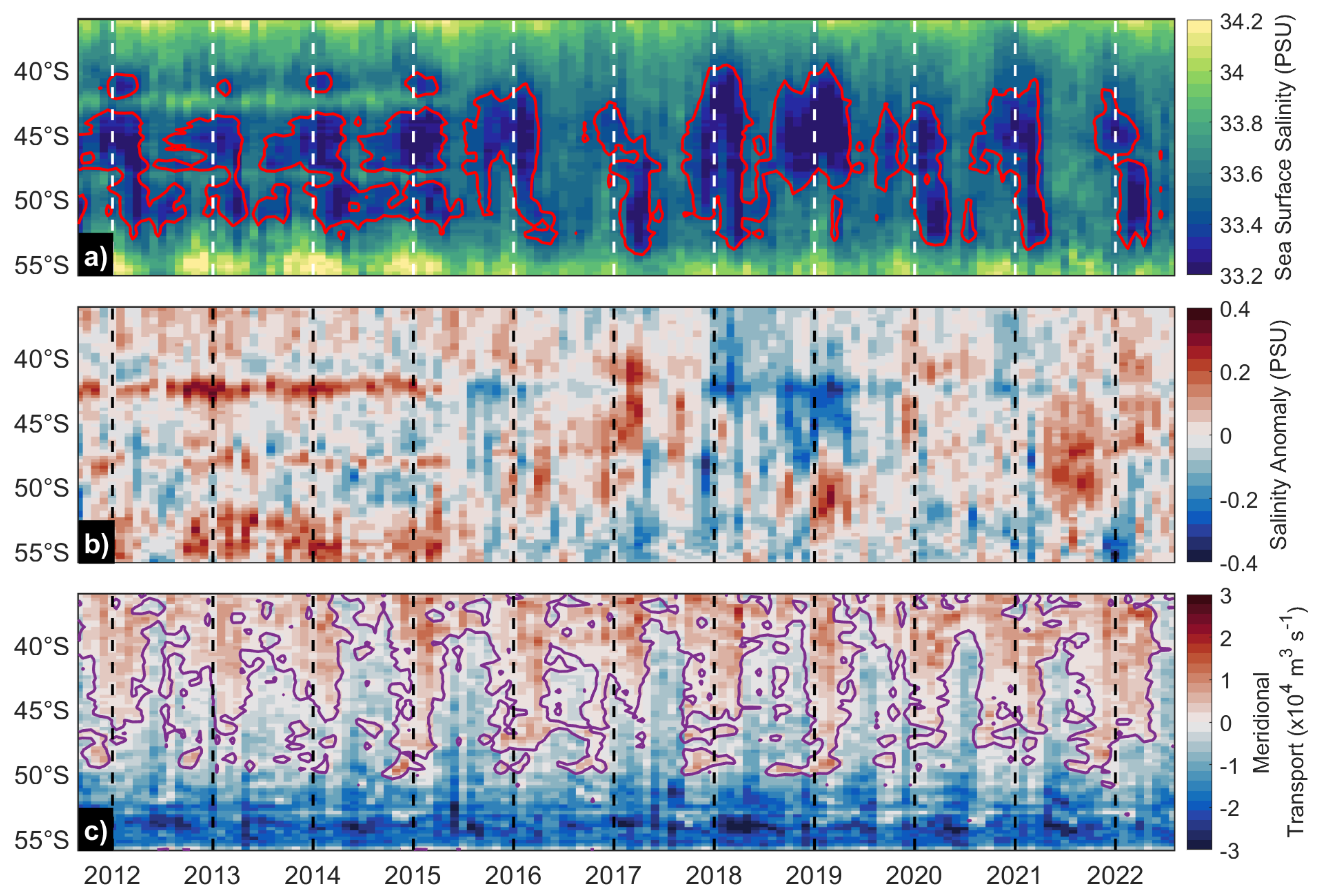
3.3. Interannual Variability of SSS, Salinity Anomalies, and Meridional Geostrophic Transports

The interannual variability of SSS along the coastal band (first 100 km) shows that salinity minima generally occur within the early months of each year. Nonetheless, there is a marked interannual variability (Figure 6a). The salinity maxima extend across the northern and southern tips of our domain. The higher salinities occurred at the southern boundary and within the first 5 years of the study (2011–2015). In contrast, the lower salinities (fresher conditions) developed during the spring–summer of 2018 and 2019. A similar SSS feature was registered by an oceanographic buoy in the Reloncaví Sound, northern Patagonia [54]. Examining the patterns of SSS anomalies (Figure 6b), we observe that higher positive anomalies occurred around 42°S (off Chiloé Island) and south of 52°S during the first 5 years (Figure 6b). The higher salinity anomalies off Chiloé Island during spring–summer could correspond to enhanced coastal upwelling events bringing cold and salty waters off northern Patagonia [36,40,55]. Reduced freshwater conditions occurred during the spring–summer of 2016–2017 and most of 2021 and 2022. On the other hand, negative anomalies prevailed during spring–summer 2015–2016 and the most of 2018 and 2019, indicating a trend towards a greater amount of freshwater during these periods. These findings complement the seasonal patterns found by Saldías et al. [9] and highlight the importance of implementing a long-term monitoring effort to further understand the implications of freshwater outflows and coastal currents off western Patagonia.

The meridional geostrophic transport shows that the annual cycle is well marked in all the years of the study (Figure 6c), with the predominant northward transport covering a larger region (it is extended further south) during the warm seasons (spring–summer). This variability may be linked to the seasonal migration of the South Pacific Gyre, which has been observed to strengthen (spin-up effect) in relation to the Southern Annual Mode [56,57]. In contrast, the southward transport reaches its northernmost latitudes during fall–winter. Anomalously, the southward geostrophic flow reached up to 39°S during the winters of 2014 and 2022 (Figure 6c). However, this anomalous northward extension does not coincide with a stronger Cape Horn Current. The stronger southward flows occurred generally south of 50°S and during 2012 and 2018.

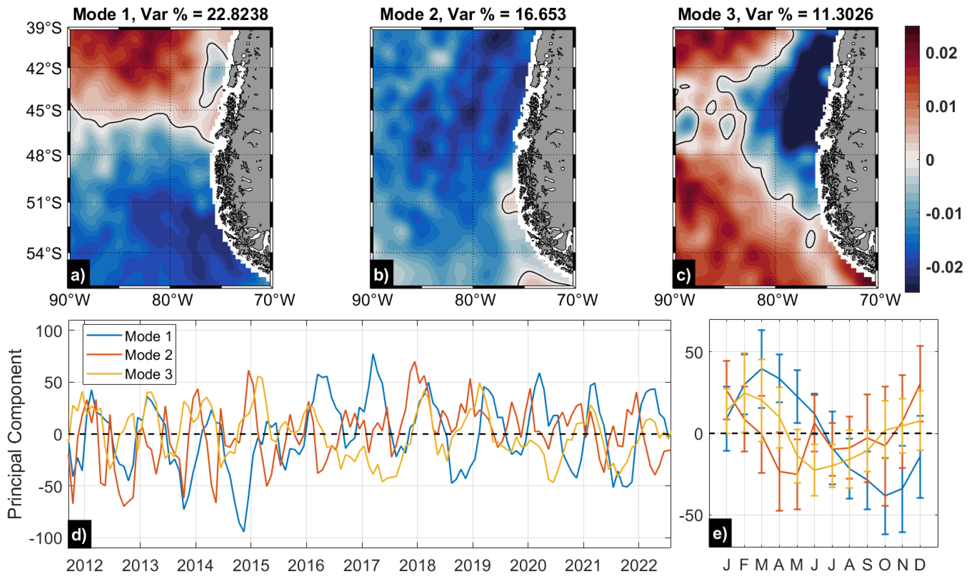
3.4. Dominant Spatio-Temporal Modes of Variability and Linear Trends

An EOF analysis using monthly normalized SSS fields is presented in Figure 7. The first three modes explain 22.8%, 16.6%, and 11.3% of the total variance, respectively. The spatial pattern of the first mode exhibits a north–south dipole, with its sign change occurring near 48°S nearshore (Figure 7a) and predominantly occurring in summer (Figure 7e). The spatial pattern of the second mode shows that most of the entire region varies together (Figure 7b), with negative anomalies mainly occurring during December and January (Figure 7e). The spatial pattern of the third mode exhibits an east–west dipole (Figure 7c), where the eastern zone shows a higher magnitude in a coastal tongue north of ∼52°S, and where the enhanced negative anomalies are presented in the coastal area north of the Gulf of Penas.

The time series associated with the first principal component represents a marked seasonal variability (Figure 7e), with preferred positive/negative anomalies for particular years (Figure 7d). This first principal component (blue curve) switched from large negative values to mostly positive values in 2016, which suggests an increase in freshwater conditions (lower salinities) with the greatest contribution during most of 2016, 2017, and 2022. Other years post-2016 (e.g., 2018, 2019, and 2021) presented a stronger seasonal pattern. This aligns with the saline minima observed during those years south of 48°S along the coastal band (Figure 6a). The time series associated with the second principal component (Figure 7d) suggests periods of increased freshwater primarily during spring and summer and in phase along the coastal band (Figure 7b). Supporting this signal, a core of minimum salinity is appreciated north of 48°S during 2018–2019 (Figure 6a), also related to the most intense negative anomalies observed (Figure 6b). The time series associated with the third principal component (Figure 7d) shows that there was an inclination towards greater salinities in a tongue north of about 51°S, such as during 2016–2017 (Figure 7c,d).

Considering the relatively large meridional extension of the study area, SSS variability could lead to contrasting patterns of long-term freshening and/or increased salinity trends. Thus, the linear trends (2011–2022) were computed for each pixel to provide a preliminary assessment of coastal areas potentially experiencing freshening. Although the 11-year time series is not long enough to provide a solid conclusion of freshening, it identifies the coastal areas off western Patagonia that are likely to continue with those long-term trends. Two main regions were identified with a decreasing SSS trend: the coastal ocean off southern Patagonia, limited to the areas south of ∼52°S and with a decreasing trend between −0.02 and −0.03 psu year⁻¹, and the coastal area off Chiloé Island (41.7–43.3°S) with a marked negative trend about −0.03 psu year⁻¹ (Figure 8). The coastal areas with the lowest salinities (greater freshwater inputs) have mainly been found off central Patagonia [8,9,22]. Nonetheless, this pattern might change in the future if these trends persist in the long-term. Eventually, the coastal ocean off southern Patagonia might become a region comparable to the fresher coastal ocean off central Patagonia, which might have profound implications for the strength and dynamics of the Cape Horn Current. In the context of climate change and variability, future studies are suggested combining in situ and satellite observation along/across the salinity gradients of the entire coastal ocean of Chilean Patagonia to further understand the impact of freshening due to global surface warming [58] on the biogeochemical cycles, and the link between the thermohaline structure (i.e., density gradients) and the dynamics of the Cape Horn Current.

References

1. Vinogradova, N.; Lee, T.; Boutin, J.; Drushka, K.; Fournier, S.; Sabia, R.; Stammer, D.; Bayler, E.; Reul, N.; Gordon, A.; et al. Satellite salinity observing system: Recent discoveries and the way forward. Front. Mar. Sci. 2019, 6, 428925. [Google Scholar] [CrossRef]
2. Piola, A.R.; Romero, S.I.; Zajaczkovski, U. Space–time variability of the Plata plume inferred from ocean color. Cont. Shelf Res. 2008, 28, 1556–1567. [Google Scholar] [CrossRef]
3. Saldías, G.S.; Largier, J.L.; Mendes, R.; Pérez-Santos, I.; Vargas, C.A.; Sobarzo, M. Satellite-measured interannual variability of turbid river plumes off central-southern Chile: Spatial patterns and the influence of climate variability. Prog. Oceanogr. 2016, 146, 212–222. [Google Scholar] [CrossRef]
4. Warrick, J.A.; Farnsworth, K.L. Coastal river plumes: Collisions and coalescence. Prog. Oceanogr. 2017, 151, 245–260. [Google Scholar] [CrossRef]
5. Mendes, R.; Saldías, G.S.; deCastro, M.; Gómez-Gesteira, M.; Vaz, N.; Dias, J.M. Seasonal and interannual variability of the Douro turbid river plume, northwestern Iberian Peninsula. Remote Sens. Environ. 2017, 194, 401–411. [Google Scholar] [CrossRef]
6. Royer, T.C. On the effect of precipitation and runoff on coastal circulation in the Gulf of Alaska. J. Phys. Oceanogr. 1979, 9, 555–563. [Google Scholar] [CrossRef]
7. Hill, A.E.; Hickey, B.M.; Shellington, F.A.; Strub, P.T.; Brink, K.H.; Barton, E.D.; Thomas, A.C. Eastern Ocean Boundaries. In The Sea: The Global Coastal Ocean, Regional Studies and Synthesis; Robinson, A.R., Brink, K.H., Eds.; John Wiley: New York, NY, USA, 1998; pp. 29–67. [Google Scholar]
8. Dávila, P.M.; Figueroa, D.; Müller, E. Freshwater input into the coastal ocean and its relation with the salinity distribution off austral Chile (35–55°S). Cont. Shelf Res. 2002, 22, 521–534. [Google Scholar] [CrossRef]
9. Saldías, G.S.; Sobarzo, M.; Quiñones, R. Freshwater structure and its seasonal variability off western Patagonia. Prog. Oceanogr. 2019, 174, 143–153. [Google Scholar] [CrossRef]
10. Jones, E.; Anderson, L.; Jutterström, S.; Swift, J. Sources and distribution of fresh water in the East Greenland Current. Prog. Oceanogr. 2008, 78, 37–44. [Google Scholar] [CrossRef]
11. Mork, M. Circulation phenomena and frontal dynamics of the Norwegian Coastal Current. Philos. Trans. R. Soc. Lond. Ser. Math. Phys. Sci. 1981, 302, 635–647. [Google Scholar]
12. Royer, T.C. Coastal fresh water discharge in the northeast Pacific. J. Geophys. Res. Ocean. 1982, 87, 2017–2021. [Google Scholar] [CrossRef]
13. Strub, P.T.; Mesĩas, J.; Montecino, V.; Rutlland, J.; Salinas, S. Coastal ocean circulation off western south America. In The Sea: The Global Coastal Ocean, Regional Studies and Synthesis; Robinson, A.R., Brink, K.H., Eds.; John Wiley: New York, NY, USA, 1998; pp. 273–313. [Google Scholar]
14. Zheng, Q.; Bingham, R.; Andrews, O. Using Sea Level to Determine the Strength, Structure and Variability of the Cape Horn Current. Geophys. Res. Lett. 2023, 50, e2023GL105033. [Google Scholar] [CrossRef]
15. Lagerloef, G.; Colomb, F.R.; Le Vine, D.; Wentz, F.; Yueh, S.; Ruf, C.; Lilly, J.; Gunn, J.; Chao, Y.; Decharon, A.; et al. The Aquarius/SAC-D mission: Designed to meet the salinity remote-sensing challenge. Oceanography 2008, 21, 68–81. [Google Scholar] [CrossRef]
16. Bao, S.; Wang, H.; Zhang, R.; Yan, H.; Chen, J. Comparison of satellite-derived sea surface salinity products from SMOS, Aquarius, and SMAP. J. Geophys. Res. Ocean. 2019, 124, 1932–1944. [Google Scholar] [CrossRef]
17. Melnichenko, O.; Hacker, P.; Potemra, J.; Meissner, T.; Wentz, F. Multi-Mission Sea Surface Salinity Optimum Interpolation (OISSS) Analysis Version 2.0; PODAAC: Pasadena, CA, USA, 2023. [Google Scholar]
18. Nardelli, B.B.; Droghei, R.; Santoleri, R. Multi-dimensional interpolation of SMOS sea surface salinity with surface temperature and in situ salinity data. Remote Sens. Environ. 2016, 180, 392–402. [Google Scholar] [CrossRef]
19. Wang, H.; Zhang, W.; Bao, S.; Chen, W.; Ren, K. Evaluation of Global Sea Surface Salinity from Four Ocean Reanalysis Products. In Proceedings of the 2022 5th International Conference on Information Communication and Signal Processing (ICICSP), Shenzhen, China, 26–28 November 2022; pp. 577–583. [Google Scholar]
20. Ouyang, Y.; Zhang, Y.; Chi, J.; Sun, Q.; Du, Y. Deviations of satellite-measured sea surface salinity caused by environmental factors and their regional dependence. Remote Sens. Environ. 2023, 285, 113411. [Google Scholar] [CrossRef]
21. Neshyba, S.; Fonseca, T.R. Evidence for counterflow to the west wind drift off South America. J. Geophys. Res. Ocean. 1980, 85, 4888–4892. [Google Scholar] [CrossRef]
22. Galán, A.; Saldías, G.S.; Corredor-Acosta, A.; Muñoz, R.; Lara, C.; Iriarte, J.L. Argo float reveals biogeochemical characteristics along the freshwater gradient off western Patagonia. Front. Mar. Sci. 2021, 8, 613265. [Google Scholar] [CrossRef]
23. Dinnat, E.P.; Le Vine, D.M.; Boutin, J.; Meissner, T.; Lagerloef, G. Remote sensing of sea surface salinity: Comparison of satellite and in situ observations and impact of retrieval parameters. Remote Sens. 2019, 11, 750. [Google Scholar] [CrossRef]
24. Reul, N.; Grodsky, S.; Arias, M.; Boutin, J.; Catany, R.; Chapron, B.; d’Amico, F.; Dinnat, E.; Donlon, C.; Fore, A.; et al. Sea surface salinity estimates from spaceborne L-band radiometers: An overview of the first decade of observation (2010–2019). Remote Sens. Environ. 2020, 242, 111769. [Google Scholar] [CrossRef]
25. Dossa, A.N.; Alory, G.; Da Silva, A.C.; Dahunsi, A.M.; Bertrand, A. Global analysis of coastal gradients of sea surface salinity. Remote Sens. 2021, 13, 2507. [Google Scholar] [CrossRef]
26. Sun, J.; Vecchi, G.; Soden, B. Sea surface salinity response to tropical cyclones based on satellite observations. Remote Sens. 2021, 13, 420. [Google Scholar] [CrossRef]
27. Melnichenko, O. Multi-Mission Optimally Interpolated Sea Surface Salinity 7-Day Global Dataset V1; PODAAC: Pasadena, CA, USA, 2021. [Google Scholar] [CrossRef]
28. Melnichenko, O.; Amores, A.; Maximenko, N.; Hacker, P.; Potemra, J. Signature of mesoscale eddies in satellite sea surface salinity data. J. Geophys. Res. Ocean. 2017, 122, 1416–1424. [Google Scholar] [CrossRef]
29. Hall, S.B.; Subrahmanyam, B.; Steele, M. The role of the Russian Shelf in seasonal and interannual variability of Arctic sea surface salinity and freshwater content. J. Geophys. Res. Ocean. 2023, 128, e2022JC019247. [Google Scholar] [CrossRef]
30. Hoffman, E.L.; Subrahmanyam, B.; Trott, C.B.; Hall, S.B. Comparison of Freshwater Content and Variability in the Arctic Ocean Using Observations and Model Simulations. Remote Sens. 2023, 15, 3715. [Google Scholar] [CrossRef]
31. Li, J.; Han, D.; Liao, G.; Zhang, T.; Ding, R.; Song, X. Dynamics of the barrier layer dipole in the equatorial Indian Ocean. J. Geophys. Res. Ocean. 2024, 129, e2023JC020479. [Google Scholar] [CrossRef]
32. Yu, L. Connecting subtropical salinity maxima to tropical salinity minima: Synchronization between ocean dynamics and the water cycle. Prog. Oceanogr. 2023, 219, 103172. [Google Scholar] [CrossRef]
33. Laurindo, L.C.; Siqueira, L.; Small, R.J.; Thompson, L.; Kirtman, B.P. Quantifying the contribution of ocean advection and surface flux to the upper-ocean salinity variability resolved by climate model simulations. Geophys. Res. Lett. 2024, 51, e2023GL106354. [Google Scholar] [CrossRef]
34. Vazquez-Cuervo, J.; Dewitte, B.; Chin, T.M.; Armstrong, E.M.; Purca, S.; Alburqueque, E. An analysis of SST gradients off the Peruvian Coast: The impact of going to higher resolution. Remote Sens. Environ. 2013, 131, 76–84. [Google Scholar] [CrossRef]
35. Saldías, G.S.; Lara, C. Satellite-derived sea surface temperature fronts in a river-influenced coastal upwelling area off central–southern Chile. Reg. Stud. Mar. Sci. 2020, 37, 101322. [Google Scholar] [CrossRef]
36. Saldías, G.S.; Hernández, W.; Lara, C.; Muñoz, R.; Rojas, C.; Vásquez, S.; Pérez-Santos, I.; Soto-Mardones, L. Seasonal variability of SST fronts in the Inner Sea of Chiloé and its adjacent coastal ocean, northern Patagonia. Remote Sens. 2021, 13, 181. [Google Scholar] [CrossRef]
37. Emery, W.J.; Thomson, R.E. Data Analysis Methods in Physical Oceanography, 2nd ed.; Elsevier: Amsterdam, The Netherlands, 2004. [Google Scholar]
38. Flores, R.P.; Lara, C.; Saldías, G.S.; Vásquez, S.I.; Roco, A. Spatio-temporal variability of turbid freshwater plumes in the Inner Sea of Chiloé, northern Patagonia. J. Mar. Syst. 2022, 228, 103709. [Google Scholar] [CrossRef]
39. Strub, P.T.; James, C.; Montecino, V.; Rutllant, J.A.; Blanco, J.L. Ocean circulation along the southern Chile transition region (38–46S): Mean, seasonal and interannual variability, with a focus on 2014–2016. Prog. Oceanogr. 2019, 172, 159–198. [Google Scholar] [CrossRef] [PubMed]
40. Pérez-Santos, I.; Seguel, R.; Schneider, W.; Linford, P.; Donoso, D.; Navarro, E.; Amaya-Cárcamo, C.; Pinilla, E.; Daneri, G. Synoptic-scale variability of surface winds and ocean response to atmospheric forcing in the eastern austral Pacific Ocean. Ocean Sci. 2019, 15, 1247–1266. [Google Scholar] [CrossRef]
41. Yu, L. A global relationship between the ocean water cycle and near-surface salinity. J. Geophys. Res. Ocean. 2011, 116. [Google Scholar] [CrossRef]
42. Aiken, C.M. Seasonal thermal structure and exchange in Baker Channel, Chile. Dyn. Atmos. Ocean. 2012, 58, 1–19. [Google Scholar] [CrossRef]
43. Ross, L.; Pérez-Santos, I.; Parady, B.; Castro, L.; Valle-Levinson, A.; Schneider, W. Glacial lake outburst flood (GLOF) events and water response in a patagonian fjord. Water 2020, 12, 248. [Google Scholar] [CrossRef]
44. Silva, N.; Sievers, H.; Prado, R. Características oceanográficas y una proposición de circulación para algunos canales Australes de Chile entre 41º20′S y 46º40′S. Rev. Biol. Mar. 1995, 30, 207–254. [Google Scholar]
45. Silva, N.; Rojas, N.; Fedele, A. Water masses in the Humboldt Current System: Properties, distribution, and the nitrate deficit as a chemical water mass tracer for Equatorial Subsurface Water off Chile. Deep Sea Res. Part II 2009, 56, 1004–1020. [Google Scholar] [CrossRef]
46. Schneider, W.; Fuenzalida, R.; Rodríguez-Rubio, E.; Garcés-Vargas, J.; Bravo, L. Characteristics and formation of eastern South Pacific intermediate water. Geophys. Res. Lett. 2003, 30, 1581. [Google Scholar] [CrossRef]
47. Linford, P.; Pérez-Santos, I.; Montes, I.; Dewitte, B.; Buchan, S.; Narváez, D.; Saldías, G.; Pinilla, E.; Garreaud, R.; Díaz, P.; et al. Recent deoxygenation of Patagonian fjord subsurface waters connected to the Peru–Chile undercurrent and equatorial subsurface water variability. Glob. Biogeochem. Cycles 2023, 37, e2022GB007688. [Google Scholar] [CrossRef]
48. Pickard, G. Some physical oceanographic features of inlets of Chile. J. Fish. Board Can. 1971, 28, 1077–1106. [Google Scholar] [CrossRef]
49. Sievers, H.; Silva, N. Water masses and circulation in austral Chilean channels and fjords. In Progress in the Oceanographic Knowledge of Chilean Interior Waters, from Puerto Montt to Cape Horn; Silva, N., Palma, S., Eds.; Comité Oceanográfico Nacional—Pontificia Universidad Católica de Valparaíso, Valparaíso: Valparaíso, Chile, 2008; pp. 53–58. [Google Scholar]
50. Pérez-Santos, I.; Garcés-Vargas, J.; Schneider, W.; Ross, L.; Parra, S.; Valle-Levinson, A. Double-diffusive layering and mixing in Patagonian fjords. Prog. Oceanogr. 2014, 129, 35–49. [Google Scholar] [CrossRef]
51. Hickey, B.M. The California current system—Hypotheses and facts. Prog. Oceanogr. 1979, 8, 191–279. [Google Scholar] [CrossRef]
52. Mazzini, P.L.; Barth, J.A.; Shearman, R.K.; Erofeev, A. Buoyancy-driven coastal currents off Oregon during fall and winter. J. Phys. Oceanogr. 2014, 44, 2854–2876. [Google Scholar] [CrossRef]
53. Cushman-Roisin, B.; Beckers, J.M. Introduction to Geophysical Fluid Dynamics: Physical and Numerical Aspects; Academic Press: Cambridge, MA, USA, 2011. [Google Scholar]
54. Pérez-Santos, I.; Díaz, P.A.; Silva, N.; Garreaud, R.; Montero, P.; Henríquez-Castillo, C.; Barrera, F.; Linford, P.; Amaya, C.; Contreras, S.; et al. Oceanography time series reveals annual asynchrony input between oceanic and estuarine waters in Patagonian fjords. Sci. Total Environ. 2021, 798, 149241. [Google Scholar] [CrossRef]
55. Narváez, D.A.; Vargas, C.A.; Cuevas, L.A.; García-Loyola, S.A.; Lara, C.; Segura, C.; Tapia, F.J.; Broitman, B.R. Dominant scales of subtidal variability in coastal hydrography of the Northern Chilean Patagonia. J. Mar. Syst. 2019, 193, 59–73. [Google Scholar] [CrossRef]
56. Qu, T.; Fukumori, I.; Fine, R.A. Spin-up of the southern hemisphere super gyre. J. Geophys. Res. Ocean. 2019, 124, 154–170. [Google Scholar] [CrossRef]
57. Hitt, N.T.; Sinclair, D.J.; Neil, H.L.; Fallon, S.J.; Komugabe-Dixson, A.; Fernandez, D.; Sutton, P.J.; Hellstrom, J.C. Natural cycles in south Pacific gyre strength and the southern annular mode. Sci. Rep. 2022, 12, 18090. [Google Scholar] [CrossRef]
58. Lee, H.; Calvin, K.; Dasgupta, D.; Krinner, G.; Mukherji, A.; Thorne, P.; Trisos, C.; Romero, J.; Aldunce, P.; Barret, K.; et al. IPCC, 2023: Climate Change 2023: Synthesis Report, Summary for Policymakers. Contribution of Working Groups I, II and III to the Sixth Assessment Report of the Intergovernmental Panel on Climate Change; Core Writing Team, Lee, H., Romero, J., Eds.; IPCC: Geneva, Switzerland, 2023. [Google Scholar]
Figure 1. Study area off western Patagonia. (a) Average and (b) standard deviation of sea surface salinity from the OISSS product (2011–2022). (c) Average surface salinity (0–10 m) from all available Argo floats in the region (8540 good-quality profiles). The vectors are the average geostrophic velocities for the same period. White contours in (a) correspond to the 33.6, 33.7, 33.8, 33.9, and 34 psu isolines, and the red line delimits the low-salinity core defined by the 33.45 isoline.
Remotesensing 16 01482 g001
Figure 2. Seasonal variability of (ad) average and (eh) standard deviation of sea surface salinity from the OISSS product (2011–2022). Seasonal variability of sea surface salinity from Argo floats (0–10 m) (il). The seasons are defined as summer (JFM), fall (AMJ), winter (JAS), and spring (OND). White contours in (ad) correspond to the 33.6, 33.7, 33.8, 33.9, and 34 psu isolines, and the red lines delimit the low-salinity core defined by the 33.45 isoline.
Remotesensing 16 01482 g002
Figure 3. Seasonal variability of river discharges for the Palena River (northern Patagonia; blue line), Baker River (central Patagonia; red line), and Serrano River (southern Patagonia; yellow line). The seasonal climatologies were computed using the period 2011–2022.
Remotesensing 16 01482 g003
Figure 4. Seasonal variability of (a) surface salinity and (b) meridional geostrophic transport as a function of latitude considering the average fields for a coastal band of 100 km. The red contour in (a) corresponds to the 33.45 psu isoline as in Figure 1 and Figure 2, and the black line in (b) denotes the zero transport isoline.
Remotesensing 16 01482 g004
Figure 5. Seasonal variability of (ad) average and (eh) standard deviation of the gradient magnitude of sea surface salinity from the OISSS product (2011–2022). The seasons are defined as summer (JFM), fall (AMJ), winter (JAS), and spring (OND).
Remotesensing 16 01482 g005
Figure 6. Interannual variability of (a) surface salinity, (b) surface salinity anomaly, and (c) meridional geostrophic transport as a function of latitude considering average fields for a coastal band of 100 km. The red contour in (a) corresponds to the 33.45 psu isoline, whereas the purple contour in (c) denotes the zero transport isoline.
Remotesensing 16 01482 g006
Figure 7. EOF analysis of sea surface salinity. (a) First, (b) second, and (c) third modes of variability. (d) EOF time series for the corresponding mode (mode 1 in blue, mode 2 in red, and mode 3 in yellow). (e) Seasonal climatology of the first three EOF time series.
Remotesensing 16 01482 g007
Figure 8. Spatial distribution of linear trends of sea surface salinity during the period 2011–2022. Positive (negative) values indicate an increase (decrease) in surface salinity.
Remotesensing 16 01482 g008
Disclaimer/Publisher’s Note: The statements, opinions and data contained in all publications are solely those of the individual author(s) and contributor(s) and not of MDPI and/or the editor(s). MDPI and/or the editor(s) disclaim responsibility for any injury to people or property resulting from any ideas, methods, instructions or products referred to in the content.