Research on Automatic Wavelength Calibration of Passive DOAS Observations Based on Sequence Matching Method

Abstract

Passive differential optical absorption spectroscopy (DOAS) is widely used to monitor the three-dimensional distribution of atmospheric pollutants. However, the observational and retrieval accuracy of this technique is significantly influenced by the precise wavelength calibration of solar spectra. Current calibration methods face challenges in automation when dealing with complex remote-sensing conditions. We introduce a novel automatic wavelength calibration algorithm for passive DOAS based on sequence-matching technology to estimate the spectral parameters of the spectrometer channels, integrating advanced processing measures such as feature structure enhancement and sub-pixel interpolation. These measures significantly reduce the dependency on reference spectrum resolution and accurately correct even minor spectral shifts. We perform sensitivity experiments using synthetic spectra to determine optimal retrieval configurations, followed by field tests at four cities on the Yangtze River Delta, China, to calibrate and compare passive DOAS instruments of various resolutions. Comparative verification in these field studies demonstrated that our algorithm was suitable for rapid spectral calibration within a wider resolution range of 0.03 nm to 0.1 nm with a wavelength inversion error < 0.01 nm. This highlights the applicability and calibration precision of our algorithm.

1. Introduction

With the rapid development of globalization and the expansion of human activities, air pollution is increasingly threatening human health and endangering the integrity of ecosystems. Therefore, monitoring the atmospheric environment is of great significance. Passive differential optical absorption spectroscopy (DOAS) is a remote sensing method used for the detection of atmospheric pollutants. It uses the differential absorption of solar radiation within various material absorption bands to quantitatively plot its atmospheric distribution [1,2,3]. With the development of remote sensing inversion algorithms, passive DOAS technology can achieve the detection of the three-dimensional distribution of pollutants, including aerosols and trace gases [4,5,6,7]. Due to its inherent non-contact characteristics, high sensitivity, wide wavelength capability, and ability to detect various components, passive DOAS has become an important pollutant detection technology on a global scale and has been recognized in international comparative verification [8,9]. With the improvement of global passive DOAS monitoring networks, the use of passive DOAS in practical environmental monitoring scenarios has increased, and case studies have become more diverse [10,11,12].

Solar radiation is the foundation of passive DOAS observations, and the accuracy of passive DOAS measurements is directly affected by solar radiation. There are currently many studies on solar radiation that greatly promote the development of passive DOAS [13,14,15,16,17,18]. In the passive DOAS observation system, the spectrometer is a key instrument in this technology, as solar radiation is mainly received by the spectrometer [6]. The spectrometer converts light signals from the sun into electrical signals, and we achieve the inversion of pollutants in different bands by combining accurate wavelength information from different channels. In order to improve the accuracy and reliability of passive DOAS measurement results, wavelength calibration methods must be precise and robust [19].

Contemporary DOAS wavelength-calibration methodologies mainly involve manual intervention, which precludes their capacity for automation. These methodologies are generally dichotomized into external light-source techniques and solar-spectrum methods. The former involves interfacing a spectrometer with a standard external light source that emits known spectral lines to derive the instrument’s response curve and accomplish wavelength referencing and calibration [20,21,22]. For example, the error can be controlled within 1.6 pm using the standard light source of a mercury lamp [22]. Despite its broad adoption because of its simplicity of operation and high-level accuracy, this technique has several intrinsic limitations. These include the need for laborious manual management of the standard light source, aligning light source conditions with established standards, and conducting rigorous spectral analysis; the necessity for disparate standard light sources across different spectral bands, resulting in non-uniformity and the potential for health risks to operators through improper use; and the likelihood of minor operational deviations in the instrument during runtime, leading to variation between actual wavelengths and those obtained under standard calibration conditions—a pervasive challenge that remains elusive to comprehensive resolution.

Solar spectrum methods, an alternative to external light-source techniques, use the standard solar spectrum as a reference to calibrate wavelength channels based on characteristic absorption, scattering, and radiative properties [23]. Favored for their ability to obviate manual calibration processes, these methods can detect and rectify marginal wavelength shifts during instrument stability. However, this approach demands an exceedingly high-resolution standard solar spectrum, constraining its application to ordinary instruments. Typically, standard spectra require a resolution of 0.001 nm with a corrected wavelength error of 0.003 nm [21]. For example, the significant difference in wavelength resolution between the standard spectrum and the measured spectrum leads to low matching terms. Furthermore, this approach does not cater to the detection of wavelength shifts across various spectral ranges, a problem frequently encountered in field observations [17,24].

In field operations, a combined methodology is often used to assure instrument stability: initial instrument pre-calibration with a standard light source, followed by ongoing adjustments using the solar spectrum throughout continuous observation cycles [25].

We wondered if the merits of both approaches could be amalgamated to accommodate complex operational conditions, sustain continuous automatic correction, and facilitate band-specific inversions. Building upon existing calibration methods, we introduce an innovative automatic solar spectrum wavelength calibration algorithm that reduces reliance on external light sources and mitigates the dependency on standard light sources. Using sequence matching technology [26], the algorithm is universally applicable, irrespective of resolution, and is executed through a four-step procedure encompassing spectral preprocessing, channel alignment, offset adjustment, and wavelength reconstruction. The algorithm integrates sophisticated feature extraction [27,28,29,30] and channel segmentation techniques, ensuring high precision and calibration accuracy devoid of elaborate external reference light sources. Moreover, it offers the flexibility to adapt to varying scenarios. This algorithm also seamlessly integrates as a compact plug-in within the DOAS observation system to facilitate real-time, high-accuracy wavelength calibration and preemptive signal anomalies during field observations. Therefore, this research fosters interest in spectral matching and data processing methodologies and propels technological advancements into atmospheric environmental monitoring.

To corroborate the efficacy of our proposed method, we demonstrate the calibration process for UV-Vis spectrometers, focusing on the UV-visible light spectrum. Section 2 elucidates the foundational principles and practical implementation of the passive DOAS calibration algorithm; Section 3 conducts experiments to assess the algorithm’s sensitivity to various parameters; Section 4 undertakes validation in a real-world field setting; and Section 5 summarizes the algorithm’s features and its potential applications.

2. Passive DOAS Wavelength Automatic Calibration Algorithm

2.1. Definition of Passive DOAS Spectral Sequence Matching

Our passive DOAS system (Figure 1) captures solar radiation with a telescope, which is then directed to a UV-Vis spectrometer via optical fibers. Our focus lies primarily on the ultraviolet to visible light spectrum. Sunlight, after passing through the spectrometer’s slit, produces a diffraction pattern that is captured and transformed into an electrical signal by a two-dimensional scanning imager, producing an output of light intensity data. This spectral information, once processed by an accompanying computer and software, allows for the inversion of detailed atmospheric pollutant information. The amount of signal captured by the spectrometer depends on channel number, with the essential data comprising light intensity and wavelength. Light intensity is directly provided by a charge-coupled device (CCD), while wavelength information requires calibration of the spectrometer’s channels.

For clarity, we establish the following notations: Spectral signals are denoted as follows:

$$S={\{(x_i,w_i,l_i)|x_1<x_2<\cdot \cdot \cdot <x_N\}}_{i=1}^N$$

(1)

where $S$ represents the signal sequence, $x_i$ are the channels, $w_i$ is the channel wavelength information, $l_i$ is the channel light intensity signal, and $N$ is the number of channels in the spectrometer. A key task of the passive DOAS system is to acquire accurate wavelength signals ($w_i$) for each channel.

The matching of spectral sequences (Figure 2) involves using a standard spectrum as a wavelength reference, aligning the channels of the measured spectrum with those of the standard spectrum through channel changes, and achieving optimal matching of light intensity sequences. The wavelength back-calculation is then performed using the wavelength calibration of the standard spectrum.

Wavelength inversion can be performed via piecewise linear interpolation. Because sunlight comprises continuous parallel beams entering the slit ($D$) collimatedly, the resulting diffraction angle $\theta$ adheres to Fraunhofer’s single-slit diffraction formula:

$$D\sin \theta =m\lambda$$

(2)

For a slit width set at about 10² μm, we deduce that at the maximum diffraction angle for each channel (P), there is a piecewise linear relationship between the ultraviolet to visible light intensity and its corresponding central wavelength ($\lambda$). Therefore, wavelength back-calculation for featured channel wavelengths can be achieved through linear interpolation [26,27].

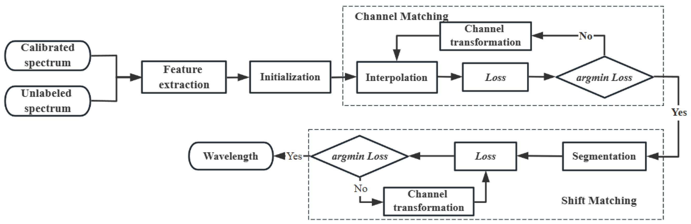
2.2. Wavelength Calibration Algorithm Based on Sequence Matching

The task of passive DOAS spectral wavelength calibration is to invert an unknown channel wavelength function through a standard spectrum. We propose a passive DOAS wavelength calibration algorithm based on sequence matching. The algorithmic process comprises four main steps (Figure 3). The first step involves input and spectral preprocessing, which includes feature extraction from the standard spectrum and the selection of matching bands to enhance the algorithm’s discriminatory power, mainly to maximize differentiation between non-matching and optimally matching channels. The second step involves spectral channel matching, wherein wavelength shifts at the channel level are corrected for two spectra. By interpolating the high-resolution spectrum to match the number of channels and using a value function, we identify the best-matching channel for the measured spectrum against a standard one. The third step addresses sub-channel level spectral drift correction, aimed at refining calibration resolution and accuracy by splitting channels identified in step two into adjacent virtual sub-channels for correction. The fourth step involves wavelength interpolation and output; full-channel wavelength computation and output are achieved through piecewise linear interpolation.

Implementation of the algorithm hinges on three key techniques: feature extraction, intensity interpolation (within and between channels), and optimal estimation. We explore these parameters and conduct sensitivity experiments to ascertain optimal parameter settings and to enhance the algorithm’s robustness.

The degree of sequence matching is determined using an evaluation function, which guides the search for the most suitable match [27,31,32,33]. The measured spectrum can be matched to the characteristic bands of the standard spectrum by interpolation, allowing for a discretized evaluation function. We use the following mean square error function:

$$Loss(l)=\frac{1}{e-s}\times {\displaystyle \sum _{j=s}^e||l_j-{\widehat{l}}_j||}$$

(3)

Interpolation enables matching any measured spectrum channel $(s,e)$ to the chosen feature band $(p,q)$ of the standard spectrum, where ${\widehat{l}}_j$ represents the result of interpolating the measured spectrum according to the interval of the reference standard $l_j$, and $(w_s,w_e)$ represents the wavelength function of the channel interval under the standard reference spectrum. The spectral channel $(p,q)$ matched to the measured spectrum can be used to calculate the wavelength function, which, under the linearity of Equation (4), can be expressed as follows:

$$w^{new}(x)=\frac{w_e-w_s}{q-p}\times (x-p)+w_s$$

(4)

The goal of the calibration algorithm inversion is to search for spectral band parameters of the measured spectrum that minimize the value function, as follows:

$$(p,q)=\underset{(p,q)}{\arg \min } Loss(l_{s\to e})$$

(5)

By solving the optimal match with Equation (5) (optimal parameter estimation of DOAS channel) and back-substituting the bands with Equation (4) (wavelength interpolation of channel), the wavelength calibration algorithm can be effectively implemented.

2.3. Algorithm Implementation and Parameter Setting

Implementation of the algorithm is predicated on the computation of the value function, which requires the spectral channel numbers of the test spectrum to match those of the standard spectrum. This requirement dictates that the test spectrum must be interpolated to conform to the number of characteristic bands in the standard spectrum. The spectral interpolation function must efficiently preserve the absorption structures in the solar spectrum (a fundamental aspect of the entire inversion process). Because the choice of interpolation function can significantly affect inversion outcomes, and given the specific absorption characteristics of the Fraunhofer structures in the solar spectrum, broadband polynomial fitting may attenuate these structures. Local interpolation is also prone to overfitting and Runge’s phenomenon [30]. Consequently, we use a piecewise interpolation approach to handle adjacent channels to ensure local absorption feature integrity. We examine three typical piecewise interpolation methods: Lagrange interpolation (LI), Hermite interpolation (HI), and spline interpolation (SI). Interpolation outcomes within adjacent channels are represented as follows:

$$\widehat{l}(x)=\left\{\begin{array}{l}\mathrm{LI}:{\displaystyle \sum _{j=i,i+1}{l}_j{L}_j(x)}\\ \mathrm{HI}:{\displaystyle \sum _{j=i,i+1}(l_j{h}_j(x)+l_j^{\prime }{H}_j(x)), x\in [x_i,x_{i+1}]}\\ \mathrm{SI}:{\displaystyle \sum _{j\in N^{+}}{a}_j}{S}_j(x^j)\end{array}\right.$$

(6)

While all three interpolation techniques are fundamentally polynomial interpolations, their fitting orders increase successively. Figure 4a presents a representation of these interpolation methods applied to raw spectral data (spectra taken as hourly averages over the observation period from 8:00–12:00 (L1) and 12:00–16:00 (L2) in the year 2023). Differences among the three interpolations are relatively minor, and the value functions remain consistent because of the closely packed spectrometer channel wavelengths and the smooth nature of the intensity function. Hence, we opt for the simplest method (Lagrange linear interpolation) for channel interpolation to reduce algorithmic complexity and enhance efficiency.

The solar spectrum’s functional relationships are inconsistent across small domains, indicating that the choice of interpolation method exerts a small impact within a narrow scope. Accordingly, we select linear interpolation for the task within these confined intervals. Nonetheless, the span of the interpolation interval remains a critical consideration because it can significantly influence interpolation accuracy and cause deviations from actual values. The results of a comparison between interpolated functions and genuine solar spectrum values using standard high-resolution solar spectra are presented in Figure 5.

Within an interpolation range of 0.02–1 nm, the solar spectrum’s performance remains stable across a 200–1000 nm wavelength range (correlation coefficient > 0.95, discrepancy < 4.3%). However, within the ultraviolet–visible (UV–visible) band, which is crucial for the inversion of atmospheric pollutant absorption cross-sections, the interpolation’s efficacy is markedly influenced by interval length. In this band, the correlation reduces to 0.5–0.6, accompanied by a near 50% relative deviation. This observation underscores the need to define an optimal interpolation interval length, which should not exceed 0.1 nm to achieve a correlation of 0.83, and the relative error should be limited to approximately 20%. Despite these findings, the impact of the interpolation interval on spectral inversion should not be a major concern. The wavelength resolution of commonly employed spectrometers typically falls below 0.1 nm, aligning with the prerequisites delineated in this analysis.

From loss function orders of magnitude, differences between observation systems, and the amplitude differences of spectra after feature enhancement are considered to be important factors affecting the solution. Considering that two factors can affect the accuracy and efficiency of the solving process, we standardize them to constrain them, as follows ($l$, ${\mu }_l$, ${\sigma }_l$, and $l_s$ represent the original intensity, mean, standard deviation, and normalized intensity data of the spectrum):

$$l_s=\frac{l-{\mu }_l}{{\sigma }_l}$$

(7)

Figure 6 illustrates the channel structures of spectra post-normalization, showing increased consistency under the same bands. The standardization process weakens amplitude differences between observation systems and enhances the consistency of signal changes. Value functions have been reduced from the order of 10⁶ to 10⁻¹, providing a basis for the reliability of subsequent optimal estimation.

In the wavelength calibration algorithm, the standard spectrum serves as a reference for sequence matching of test spectra, and feature extraction and initialization are instrumental in maximizing the algorithm’s channel discrimination capability. We devise four typical feature extraction techniques, as follows:

$$l_F(x)=\left\{\begin{array}{l}ICM: l_0(x)\\ PFM:\left\{\begin{array}{l}{l}_0(x_i), \Delta l_{+}\times \Delta l_{-}<0\\ 0, else\end{array}\right.\\ DGM :l_i-l_{i-1}\\ \begin{array}{l}SEM-pf:\begin{array}{c}\end{array}ICM\times PFM\\ SEM-dg:ICM\times DGM\end{array}\end{array}\right.$$

(8)

Feature extraction methods comprise the following: (1) an in-situ correlation method (ICM), which retains the original intensity features and uses cross-correlation analysis between standard and to-be-calibrated spectra; (2) a peak-fitting method (PFM) that focuses on identifying the largest peak within the standard spectrum and extracting its characteristics; (3) a domain gradient method (DGM) that derives gradient features from changes in intensity signals across channels and uses these gradient sequences for matching; and (4) structural enhancement methods (SEM) that enhance absorption structures through non-linear transformations of the original signal. We use two enhancement approaches based on gradient (SEM-dg) and peak value (SEM-pf). To ensure consistency of magnitudes and narrowing of the value function range for convergence in subsequent solutions, features are uniformly normalized post-extraction.

Figure 7 presents a comparison of the four feature extraction techniques against the in-situ spectra, where normalized outcomes highlight significant feature enhancement in contrast to the original spectra, with feature values amplified relative to the original signals. Gradient-based extractions (DGM, SEM-dg) introduce negative gradients to expand the spectral range and enhance trough structures. Techniques based on peak enhancement (PFM, SEM-pf) capture spectral extremities, accentuating peak structures.

The resolution of Equation (8) falls within the purview of optimal estimation theory, which, for discrete data, is typically approached through iterative algorithms, exhaustive methods, dynamic programming, or Nelder–Mead techniques, among others. These methods differ in efficiency and performance and are also influenced by spectral structures. This content is further discussed in Section 3.

3. Sensitivity Testing of Algorithm Parameters

3.1. Synthetic Spectra Based on the Standard Reference Spectrum

Parameter sensitivity experiments specific to an algorithm are performed to explore the impacts of feature extraction, channel interpolation, spectral shift, normalization, and optimization core processes in the algorithmic framework to derive the optimal configuration for inversion.

Because intrinsic differences between instruments can interfere with parameter selection, we opt to test parameters using synthetic data. Synthetic data, having a priori properties, facilitates calibration testing under known actual wavelength conditions, leading to more accurate parameter choices. The optimal parameters obtained can then benefit the calibration of subsequently measured spectra. This paper uses high-resolution solar spectra with a resolution of 0.001 nm [21].

The definition of synthetic data involves using standard spectral data to transform channels and synthesize new spectral data. According to Equation (3), both the standard and test spectra received by the spectrometer have a linear wavelength-channel correspondence, enabling linear transformations to be performed on the channels to generate new test spectra. To simulate instrumental noise, we introduce Gaussian noise; the expression for the synthetic spectrum is written as follows:

$$l_{(x\prime )}^{new}=l_{(Ax)}+\epsilon , A=(k,b), \epsilon ~N(\mu ,{\sigma }^2)$$

(9)

Because passive DOAS typically uses UV-Vis spectrometers with detection bands ranging from 200 to 400 nm and slit widths concentrated on the 10⁻¹ to 10⁻² μm scale, the magnitude of the linear transformation slope is relatively small. We select a linear transformation amplitude range of $k\in (0.9,1.1)$. After statistical analysis of the instrument’s dark current, a Gaussian distribution within the interval $l_{Guassian}=l+\epsilon \times l,\epsilon ~N(\mu ,{\sigma }^2)$ is deemed to be suitable for this instrument. Figure 8 presents a comparison of synthetic data and standard spectra, revealing significant differences at the channel level, with only similar structures in the high signal-to-noise ratio central bands, yet with notable differences in light intensity distribution. At the wavelength level, synthetic spectra display consistent distribution features with original spectra, indicating that synthetic spectra maintain wavelength stability and channel variability.

3.2. Parameter Sensitivity Experiments

Parameter sensitivity experiments using synthetic data were performed. The algorithm provides global results of the inversion process through a brute-force search. We introduce substantial noise ($\epsilon ~(0,20)$) to the signal and allow the computer to randomly simulate the linear transformation matrix, enabling the algorithm to solve the synthetic spectrum’s wavelength.

Figure 9 illustrates the algorithmic implementation process established through a brute-force search, demonstrating that feature engineering ensures algorithm performance. All provide optimal channel response relations that match randomly simulated matrices. Specifically, feature extraction offers a significant gain to algorithm implementation, resulting in more pronounced discrimination during the optimization process compared with the original spectrum (ORI). The indistinct minimum value separation in the original spectrum could lead to channel misalignment and erroneous inversion outcomes, which feature extraction ameliorates. Peak-based feature extraction increases the differential to about 0.8, while gradient-based methods only achieve 0.6. However, because structural enhancement methods do not offer better discrimination than individual features, our subsequent inversions use both gradient- and peak-based extraction methods.

To investigate the impact of selected spectral bands on the algorithm, and following feature extraction with DGM, the choice of calibration spectral bands affects the inversion (Figure 10). Loss is maintained between 0.14 and 0.19, indicating that the inversion of the state matrix for linear transformations is unaffected by channel. This allows for correct wavelength function recovery for each channel, with correlation coefficients of 1.0.

Synthetic data experiments reveal the algorithm to effectively invert linear matrices. However, this process omits the inversion of spectral drift, which is realized in the third part of the algorithm. While spectral drift is common in practical inversion processes, drift magnitude does not necessarily cause inter-channel differences, with the main offsets still being slight inter-channel deviations (addressed in step two, Section 2.2). Therefore, channel segmentation and interpolation are necessary to detect sub-channel level drift. Assuming a spectral segmentation quantity of $S$, the theoretical maximum discrepancy in spectral calibration would be ($\Delta w/2S$). We simulate various random channel values to test algorithm performance.

Figure 11 presents the effectiveness of the wavelength drift calibration process, where the algorithm can effectively retrieve randomly simulated offsets, and this inversion is applicable to any feature engineering. By examining the absolute value of wavelength shift in the range (−0.5, 0.5), the maximum value (0.04999456 of channel) is <$\Delta w/2S$, confirming that the process can achieve any predetermined level of discrimination.

Finally, we discuss the process of channel transformation in optimization of loss, which is the method of optimization for optimal estimation. From Figure 9, feature engineering effectively secures the discrimination needed for the algorithm’s optimal matching. However, it also produces an overall gradient that is less indicative of the original features, leading to a lack of direction for iterative convergence in the optimization process. Therefore, optimization of this algorithm requires a combination of the original spectrum features for coarse iteration to acquire the possible regions of the optimal solution. Following this, feature-extraction methods delineate detailed value function distributions within the scope to solve for the optimum (gradient descent and traversal: GD-T). The GD-T method has successfully narrowed the scope of a brute-force search, accelerating the algorithm’s execution efficiency.

We also investigated the selected traversal (ST) solution through the choice and optimization of traversal channels. Figure 12 compares the implementation and efficiency of ST and GD-T. The combination of iterative and brute-force search methods (GD-T) enhances efficiency by 60.8% through iteration of original features to obtain the best solution, albeit with the challenge of choosing iterative steps. The channel-selected algorithm (ST) improves efficiency by 51.0% through channel pruning. We favor the ST-optimization method because GD-T optimization depends heavily on the choice of step size, where unsuitable steps can lead to lower efficiency and the potential for erroneous inversion. Because the observation cycle usually takes a few minutes, the efficiency of both algorithms can ensure self-correction within each observation cycle. Additionally, in continuous observations, the range of wavelength drift is small, which greatly reduces the range traversed by the ST algorithm, leading to higher efficiency.

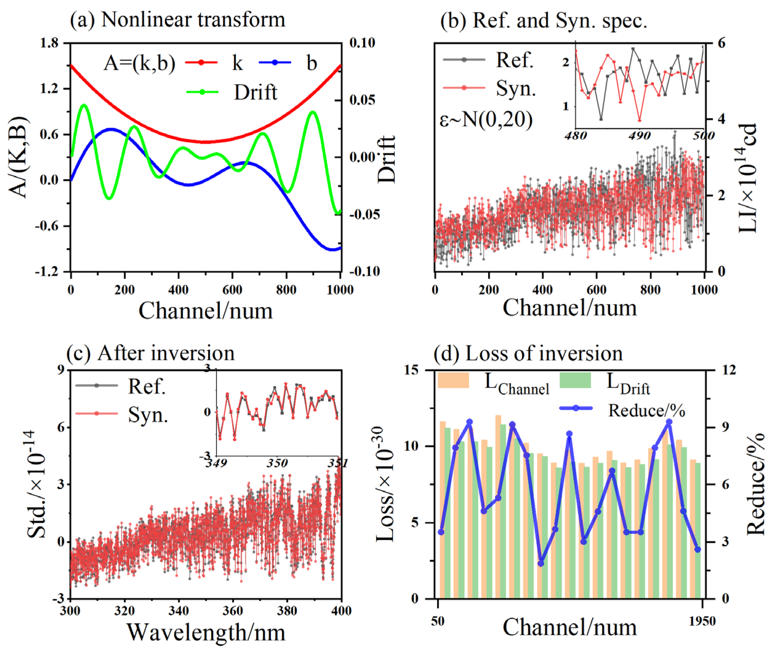
3.3. Comprehensive Inversion under Complex Transformations

We embarked on a complex synthetic data inversion experiment. Because the central wavelengths of spectrometer imaging bands usually exhibited minor shifts while edge channels showed greater deviations, we used a nonlinear function (a quadratic function increasing from center to edge) for channel transformation of synthetic spectra. We also incorporated substantial Gaussian random noise ($x~N(0,20)$) to simulate the system’s dark current noise. A spectral shift function, comprising a combination of quadratic and sine functions, was also used to simulate minor spectral shifts. Figure 13a,b illustrate the functions for these complex synthetic data variations. In our calibration process, we used a segmented approach, conducting wavelength calibration every 100 channels. As shown in Figure 13c, through dual corrections for channel and spectral shifts, we confined the loss across the full bandwidth to within 1.13 × 10⁻²⁹, with the central band, where the signal-to-noise ratio was highest, having a loss of only 8.58 × 10⁻³⁰. Sub-channel interpolation significantly contributed to loss reduction, further decreasing it by 1.8–9.2%. Figure 13d compares the channel transformation functions derived from our algorithm with the original functions, with maximum and minimum errors < 0.0032 nm and <0.0004 nm, respectively. Compared to a standard spectrum resolution of 0.01 nm, these inversion results achieved an average channel wavelength error < 10% of the resolution, indicating that our algorithm’s performance was excellent for addressing complex calibration challenges.

Our parameter sensitivity experiments for our algorithm established the optimal inversion configuration. We use a differential gradient method (DGM) for feature extraction, set the segmentation for spectral shift parameters to 1000, and optimize the channel transformation using the ST method to ensure spectral calibration accuracy. The efficiency of the algorithm guarantees that spectral self-calibration can be achieved within an observational cycle.

4. Application of Wavelength Calibration in Practical Remote Sensing

Following parameter sensitivity analyses, field-based remote sensing experiments were performed. Six solar-spectral-detection instruments were deployed across four cities (Figure 14: Lu’an, Hefei, Nanjing, and Shanghai) within the Yangtze River Delta region, China. These sites were chosen for their representation of diverse urban and rural landscapes, with distances between them ranging from 72 to 473 km. The instrumentation suite comprised a MAX-DOAS, Mobile MAX-DOAS, and CE-318 solar photometer, each offering unique spectral sampling capabilities.

Significant spectral sampling differences exist among instrumentations. The MAX-DOAS instrument captured solar spectra across various observational elements by adjusting the telescope’s elevation angle (1°, 2°, 3°, 4°, 5°, 6°, 8°, 15°, 30°, 90°), conducting spectral sampling (280–430 nm) in a stepwise fashion to ensure consistent imaging areas across all observational elements. Mobile MAX-DOAS used detectors with multiple elevation angles and optical fibers, which simultaneously transmit spectral signals to different regions of a two-dimensional CCD (1024 × 2048 pixels). The CE-318 uses a sub-band sampling method, selecting specific bands (for example, 340, 380, 440, 500, 670, 870, 1020 nm) to ascertain aerosol optical depth (AOD).

4.1. Wavelength Calibration under Different References

We calibrate wavelength and validation efforts using four passive DOAS instruments in four cities. Calibration used standard solar spectra (with a resolution of 0.01 nm) and standard mercury-lamp sources as references.

Our validation process is depicted in Figure 15. The distribution of average observations in 2023 for these instruments across the four cities, viewed from a channel perspective, is depicted in Figure 15a. Significant differences in wavelength functions among instruments existed (each observed different wavelength ranges). Hence, calibration was performed focusing on the central channel (500–1500 pixels). Figure 15b depicts the results of wavelength calibration for these spectrometers using a standard mercury-lamp source, identifying the wavelength ranges of M1 and M2 as approximately 290–390 nm and M5 and M6 as 280–420 nm. A subplot provides the distribution of values in the normalized 340–360 nm band, showing good consistency. These results also serve as true wavelength functions to compare with subsequent calibration outcomes.

Figure 15c presents calibration results using standard solar spectra and compares them with results from (b), calculating the maximum wavelength error across channels. Using solar spectra as a reference, the spectral inversion error was <0.01 nm, indicating that the sequence-matching algorithm achieved a calibration resolution below the reference spectrum resolution. Instruments with similar detection bands have similar detection accuracy. M1 and M2, with narrower wavelength ranges, perform better because of reduced influence from the interpolation function (with errors < 4 × 10⁻⁴ nm). Figure 15d compares the pairwise calibration among instruments against actual results and reveals the algorithm’s consistency. No anomalies occur when the reference spectrum matches the spectrum under test. However, the pairwise calibration process is not entirely reversible, mainly because of the selection of different channel wavelengths. This outcome suggests that using higher-resolution spectra for interpolation is beneficial and can further reduce error.

4.2. Wavelength Calibration of Mobile MAX-DOAS

Mobile MAX-DOAS was originally developed to address two major challenges in stereoscopic monitoring of atmospheric pollutants from mobile platforms: (1) Mobile-DOAS can typically observe at a single angle at any time, leading to a lack of three-dimensional distribution information about point sources and only vertical column densities within the observed area; and (2) the lengthy observation cycle of MAX-DOAS, which is inadequate for monitoring rapidly moving platforms.

Mobile MAX-DOAS uses telescopes fixed at multiple elevation angles (with the M4 model setting angles at: 1°, 2°, 3°, 4°, 5°, 6°, 8°, 15°, 30°, and 90°) to receive sunlight, which is then transmitted through respective optical fibers to a high-resolution (0.03 nm) two-dimensional spectrometer (M4: 1024 × 2048) for simultaneous imaging. However, this leads to significant differences in the offsets of different observation channels, making data assimilation and wavelength calibration for Mobile MAX-DOAS challenging. Conventional calibration methods struggle to meet the demands for multi-channel, multi-offset, high-resolution, and real-time rapid calibration of Mobile MAX-DOAS.

Our sequence matching algorithm is basically a data-assimilation method that solves this practical remote sensing challenge.

Table 1. Wavelength calibration of Mobile MAX-DOAS based on the MAX-DOAS spectrum.

EAs(θ)	1°	2°	3°	4°	5°	6°	8°	15°	30°	90°
Cha.s.pixel	502	502	502	502	501	501	501	501	502	502
Cha.e.pixel	1226	1226	1226	1226	1226	1225	1225	1226	1226	1226
Drifts.sub-pixel	0.234	0.142	0.038	0.129	0.261	0.355	0.674	0.582	0.632	0.173
Drifte.sub-pixel	0.062	0.615	0.348	0.257	0.199	0.652	0.544	0.135	0.266	0.012
Diff.MAX/10−3 nm	6.4	7.2	5.3	4.3	1.6	2.5	1.9	2.8	4.6	3.9

Ref. M2, Cha. = (500, 1500), Wave. = (317.7798, 361.6379), S = 1000.

presents calibration results based on passive DOAS (M2). It reveals that, despite significant differences in zenith angles, the inversion results are highly stable. Calibration results have a maximum error < 0.01 nm compared with standard mercury-lamp calibration wavelengths, with central band errors as low as 0.0016 nm. This clearly meets the resolution requirements for absorption cross-section fitting in spectral inversion (typically 0.5 nm). Additionally, the algorithm differentiates the wavelength offset differences across 10 elevation angles, clearly illustrating the offset disparities between central and edge channels. This demonstrates the algorithm’s broad applicability for complex high-resolution spectral correction and assimilation.

When encountering higher-resolution challenges, only two aspects need to be ensured: (1) the standard reference spectrum must be accurate, and (2) interpolation should be performed from a lower to a higher resolution using the standard spectrum as a reference.

4.3. Comparison of Spectral Inversion Products

We expand the application scope of our algorithm beyond spectral calibration verification to include data assimilation of spectra from diverse sources, corroborated by results from other monitoring devices. Using data from MAX-DOAS (M2) to conduct spectral assimilation for Mobile MAX-DOAS (M4), we map the spectral bands of Mobile MAX-DOAS onto those of MAX-DOAS to achieve congruent distributions. Spectra with matched resolutions were then processed through QDOAS inversion software (version 3.2) to extract AOD [31,32] and the temporal sequence of the pollutant component NO₂. Cross-validation among M2–4 instruments was performed to affirm method viability. Outcomes, depicted in Figure 16, reveal that post-normalization using the calibration algorithm, the spectral consistency between M2 and M4 for identical spectral bands is high. Results, post-fitting through QDOAS [33], also demonstrate significant coherence, with the dSCD inversion for NO₂ exhibiting a consistency of 0.996 and a slope of 0.966. The O₄ dSCD inversion results have a correlation of 0.994 and a slope of 0.974, and the AOD comparison with CE-318 (360 nm) yields a correlation of 0.869. These findings indicate that the automated calibration algorithm can assimilate spectral data across instruments of varying resolutions.

5. Conclusions

Our research was driven by the need to develop a channel wavelength calibration algorithm with broad applicability for automatic spectral calibration within passive DOAS systems. The algorithm reduces the resolution requirements of standard spectra and minimizes dependency on these resolutions through sequence matching. This method utilizes Fraunhofer absorption features in the solar spectrum for wavelength inversion. It achieves wavelength calibration of the measured spectra. This is performed by searching for the best match with standard spectral channel sequences.

The passive DOAS wavelength auto-calibration algorithm encompasses data pre-processing, spectral channel matching, spectral shift correction, and wavelength function interpolation. Sensitivity tests with synthetic spectra optimized the selection of key parameters. Research on feature extraction demonstrated that data processing based on peaks or gradients enhanced the clarity of optimal matches by 20–40%, with data normalization further improving feature extraction and loss convergence. In spectral channel matching, we concluded that inversion based on any characteristic channel correlated perfectly (1.0) with synthetic data, validating the effectiveness of feature extraction spectral processing methods in channel matching. For spectral shift correction, the introduction of segmented parameters ($S$) significantly reduced the variance between channel wavelength functions, enhancing wavelength detection precision by approximately 5%. Additionally, we explored optimized channel conversion strategies, where a proposed GD-T algorithm, combining gradient descent and local traversal, improved efficiency by 61% over global search solutions, and the ST (Spectral Transformation) strategy further increased efficiency by 51%. These sensitivity experiments confirmed our algorithm’s effectiveness in synthetic data wavelength inversion, verified through wavelength calibration under complex scenarios with fully non-linear transformations, achieving inversion errors < 0.01 of the reference spectrum resolution.

After obtaining optimal parameter configurations, we performed extensive remote-sensing validation over large areas, with cross-validation among instruments in four cities. Field validation of the algorithm’s measured spectra was performed using passive DOAS instruments of various resolutions, achieving self-calibration and inter-calibration of wavelengths and verifying the use of mercury-lamp spectral lines. Results indicate that our algorithm significantly captures strong Fraunhofer structures in the solar spectrum, achieving precise calibration under various reference spectra. Moreover, the algorithm facilitated simultaneous calibration of multiple channels in Mobile MAX-DOAS with a unified reference spectrum, achieving ultra-high resolution and multi-channel precise calibration. The algorithm’s inversion results for different elevation angles were stable, with mercury-lamp calibration errors < 0.01 nm. We also explored the algorithm’s data assimilation capabilities. By standardizing the wavelength distribution of two instruments using standard spectra and then inverting the spectra, aerosol states and pollutant gas information were obtained. The sequence matching-based algorithm effectively implemented spectral assimilation, with post-assimilation spectral inversion products reaching a correlation > 0.99 and validation against CE-318 also achieving a correlation > 0.86. These findings underscore the applicability, accuracy, and superiority of our algorithm. We intend to further explore the inversion resolution limits of the algorithm and delve deeper into its efficiency, striving to contribute to the field of remote sensing.

References

1. Platt, U.; Perner, D.; Pätz, H.W. Simultaneous measurement of atmospheric CH2O, O3, and NO2 by differential optical absorption. J. Geophys. Res. Ocean. 1979, 84, 6329–6335. [Google Scholar] [CrossRef]
2. Hönninger, G.; von Friedeburg, C.; Platt, U. Multi axis differential optical absorption spectroscopy (MAX-DOAS). Atmos. Chem. Phys. 2004, 4, 231–254. [Google Scholar] [CrossRef]
3. Platt, U.; Stutz, J. Differential Optical Absorption Spectroscopy. In Physics of Earth and Space Environments; Springer: Berlin, Germany, 2008. [Google Scholar] [CrossRef]
4. Rodgers, C.D. Inverse Methods for Atmospheric Sounding-Theory and Practice. In Series on Atmospheric Oceanic and Planetary Physics; World Scientific Publishing Co.: Singapore, 2000. [Google Scholar] [CrossRef]
5. Wagner, T.; Dix, B.; Friedeburg, C.V.; Frieß, U.; Sanghavi, S.; Sinreich, R.; Platt, U. MAX-DOAS O4measurements: A new technique to derive information on atmospheric aerosols-Principles and information content. J. Geophys. Res. Atmos. 2004, 109, D22. [Google Scholar] [CrossRef]
6. Sinreich, R.; Frieß, U.; Wagner, T.; Platt, U. Multi axis differential optical absorption spectroscopy (MAX-DOAS) of gas and aerosol distributions. Faraday Discuss. 2005, 130, 153. [Google Scholar] [CrossRef]
7. Zheng, J.; Xie, P.; Tian, X.; Xu, J.; Li, A.; Ren, B.; Hu, F.; Hu, Z.; Lv, Y.; Zhang, Z.; et al. McPrA-A new gas profile inversion algorithm for MAX-DOAS and apply to 50 m vertical resolution. Sci. Total Environ. 2023, 901, 165828. [Google Scholar] [CrossRef] [PubMed]
8. Kreher, K.; Van Roozendael, M.; Hendrick, F.; Apituley, A.; Dimitropoulou, E.; Frieß, U.; Richter, A.; Wagner, T.; Lampel, J.; Abuhassan, N.; et al. Intercomparison of NO2, O4, O3 and HCHO slant column measurements by MAX-DOAS and zenith-sky UV–visible spectrometers during CINDI-2. Atmospheric Meas. Tech. 2020, 13, 2169–2208. [Google Scholar] [CrossRef]
9. Tirpitz, J.-L.; Frieß, U.; Hendrick, F.; Alberti, C.; Allaart, M.; Apituley, A.; Bais, A.; Beirle, S.; Berkhout, S.; Bognar, K.; et al. Intercomparison of MAX-DOAS vertical profile retrieval algorithms: Studies on field data from the CINDI-2 campaign. Atmos. Meas. Tech. 2021, 14, 1–35. [Google Scholar] [CrossRef]
10. Wang, P.; Richter, A.; Bruns, M.; Burrows, J.P.; Scheele, R.; Junkermann, W.; Heue, K.-P.; Wagner, T.; Platt, U.; Pundt, I. Airborne multi-axis DOAS measurements of tropospheric SO2 plumes in the Po-valley, Italy. Atmos. Chem. Phys. 2010, 6, 329–338. [Google Scholar] [CrossRef]
11. Tuckermann, M.; Ackermann, R.; Gölz, C.; Lorenzen-Schmidt, H.; Senne, T.; Stutz, J.; Trost, B.; Unold, W.; Platt, U. DOAS-observation of halogen radical-catalysed arctic boundary layer ozone destruction during the ARCTOC campaigns 1995 and 1996 in Ny-Ålesund, Spitsbergen. Tellus B Chem. Phys. Meteorol. 2012, 49, 533. [Google Scholar] [CrossRef]
12. Wu, F.; Xie, P.; Li, A.; Mou, F.; Chen, H.; Zhu, Y.; Zhu, T.; Liu, J.; Liu, W. Investigations of temporal and spatial distribution of precursors SO2 and NO2 vertical columns in the North China Plain using mobile DOAS. Atmos. Chem. Phys. 2018, 18, 1535–1554. [Google Scholar] [CrossRef]
13. Wagner, T.; Beirle, S.; Dörner, S.; Penning de Vries, M.; Remmers, J.; Rozanov, A.; Shaiganfar, R. A new method for the absolute radiance calibration for UV–vis measurements of scattered sunlight. Atmos. Meas. Tech. 2015, 8, 4265–4280. [Google Scholar] [CrossRef]
14. Wagner, T.; Beirle, S.; Deutschmann, T. Three-dimensional simulation of the Ring effect in observations of scattered sun light using Monte Carlo radiative transfer models. Atmos. Meas. Tech. 2010, 2, 113–124. [Google Scholar] [CrossRef]
15. Wagner, T.; Beirle, S.; Deutschmann, T.; Penning de Vries, M. A sensitivity analysis of Ring effect to aerosol properties and comparison to satellite observations. Atmos. Meas. Tech. 2010, 3, 1723–1751. [Google Scholar] [CrossRef]
16. Deutschmann, T.; Beirle, S.; Frieß, U.; Grzegorski, M.; Kern, C.; Kritten, L.; Platt, U.; Prados-Román, C.; Wagner, T.; Werner, B.; et al. The Monte Carlo atmospheric radiative transfer model McArtim: Introduction and validation of Jacobians and 3D features. J. Quant. Spectrosc. Radiat. Transf. 2011, 112, 1119–1137. [Google Scholar] [CrossRef]
17. Woods, T.N.; Snow, M.; Harder, J.; Chapman, G.; Cookson, A. A Different View of Solar Spectral Irradiance Variations: Modeling Total Energy over Six-Month Intervals. Sol. Phys. 2015, 290, 2649–2676. [Google Scholar] [CrossRef] [PubMed]
18. Chance, K.V.; Spurr, R.J.D. Ring effect studies: Rayleigh scattering, including molecular parameters for rotational Raman scattering, and the Fraunhofer spectrum. Appl. Opt. 1997, 36, 5224. [Google Scholar] [CrossRef] [PubMed]
19. Liu, D.; Hennelly, B.M. Improved Wavelength Calibration by Modeling the Spectrometer. Appl. Spectrosc. 2022, 76, 1283–1299. [Google Scholar] [CrossRef] [PubMed]
20. Beirle, S.; Lampel, J.; Lerot, C.; Sihler, H.; Wagner, T. Parameterizing the instrumental spectral response function and its changes by a super-Gaussian and its derivatives. Atmos. Meas. Tech. 2017, 10, 581–598. [Google Scholar] [CrossRef]
21. Chance, K.; Kurucz, R.L. An improved high-resolution solar reference spectrum for earths atmosphere measurements in the ultraviolet, visible, and near infrared. J. Quant. Spectrosc. Radiat. Transf. 2010, 111, 1289–1295. [Google Scholar] [CrossRef]
22. Wu, H.; Zheng, C.; Zhang, Q.; Liu, Z.; Liang, F.; Feng, G. Calibration of mercury lamp wavelength. Optical Precision Manufacturing, Testing, and Applications. In Proceedings of the Optical Precision Manufacturing, Testing, and Applications, Beijing, China, 22–24 May 2018. [Google Scholar] [CrossRef]
23. Sun, C.; Wang, M.; Cui, J.; Yao, X.; Chen, J. Comparison and analysis of wavelength calibration methods for prism–Grating imaging spectrometer. Results Phys. 2019, 12, 143–146. [Google Scholar] [CrossRef]
24. Yu, C.; Yang, J.; Wang, M.; Sun, C.; Song, N.; Cui, J.; Feng, S. Research on spectral reconstruction algorithm for snapshot microlens array micro-hyperspectral imaging system. Opt. Express 2021, 29, 26713. [Google Scholar] [CrossRef] [PubMed]
25. Yuan, L.; Qiu, L. Wavelength calibration methods in laser wavelength measurement. Appl. Opt. 2021, 60, 4315. [Google Scholar] [CrossRef] [PubMed]
26. Yazdani, N.; Ozsoyoglu, Z.M. Sequence matching of images. In Proceedings of the 8th International Conference on Scientific and Statistical Data Base Management, Stockholm, Sweden, 18–20 June 1996. [Google Scholar] [CrossRef]
27. Li, H.; Liang, Y.; Xu, Q.; Cao, D. Key wavelengths screening using competitive adaptive reweighted sampling method for multivariate calibration. Anal. Chim. Acta 2009, 648, 77–84. [Google Scholar] [CrossRef] [PubMed]
28. Pei, S.C.; Cheng, C.M. Extracting color features and dynamic matching for image database retrieval. IEEE Trans. Circuits Syst. Video Technol. 1999, 9, 501–512. [Google Scholar] [CrossRef]
29. Chen, Y.; Jiang, H.; Li, C.; Jia, X.; Ghamisi, P. Deep Feature Extraction and Classification of Hyperspectral Images Based on Convolutional Neural Networks. IEEE Trans. Geosci. Remote Sens. 2016, 54, 6232–6251. [Google Scholar] [CrossRef]
30. Faber, N.M.; Rajkó, R. How to avoid over-fitting in multivariate calibration—The conventional validation approach and an alternative. Anal. Chim. Acta 2007, 595, 98–106. [Google Scholar] [CrossRef] [PubMed]
31. Thalman, R.; Volkamer, R. Temperature dependent absorption cross-sections of O2–O2 collision pairs between 340 and 630 nm and at atmospherically relevant pressure. Phys. Chem. Chem. Phys. 2013, 15, 15371. [Google Scholar] [CrossRef] [PubMed]
32. Che, H.; Zhang, X.; Chen, H.; Damiri, B.; Goloub, P.; Li, Z.; Zhang, X.; Wei, Y.; Zhou, H.; Dong, F.; et al. Instrument calibration and aerosol optical depth validation of the China Aerosol Remote Sensing Network. J. Geophys. Res. Atmos. 2009, 114, 1130. [Google Scholar] [CrossRef]
33. Danckaert, T.; Fayt, C.; Roozendael, M.; Smedt, I.; Letocart, V.; Merlaud, A.; Pinardi, G. QDOAS Software User Manual; QDOAS: Uccle, Belgium, 2016. [Google Scholar]
Figure 1. Passive differential optical absorption spectroscopy (DOAS) schematic and its spectral signals.
Remotesensing 16 01485 g001
Figure 2. Sequence matching problem for wavelength calibration.
Remotesensing 16 01485 g002
Figure 3. Flow of passive differential optical absorption spectroscopy (DOAS) wavelength automatic calibration algorithm based on sequence-matching.
Remotesensing 16 01485 g003
Figure 4. Piecewise interpolation methods: Lagrange interpolation (LI), Hermite interpolation (HI), and Spline interpolation (SI). And take two spectra and display their interpolation differences through the loss function.
Remotesensing 16 01485 g004
Figure 5. Characterization of the consistency between spectral interpolation and real spectra under different interpolation interval lengths.
Remotesensing 16 01485 g005
Figure 6. Sequence standardization and its sensitivity characterization (three vertical quantities represent the loss between the spectrum and the coordinate axis, as well as loss between spectra).
Remotesensing 16 01485 g006
Figure 7. Comparison of (a) in-situ correlation (ICM), peak-fitting (PFM), domain gradient (DGM), and structural enhancement (SEM) methods and (b) their loss functions.
Remotesensing 16 01485 g007
Figure 8. Comparison of synthesized and raw data, showing distribution characteristics through two methods: channel (a) and wavelength (b).
Remotesensing 16 01485 g008
Figure 9. Spectral channel matching under different feature engineering: (a) loss of channel matching, and (b), discrimination of minimum loss.
Remotesensing 16 01485 g009
Figure 10. Impact of inversion band on inversion results: (a) characteristic band and its loss, and (b) channel response (retrieved linear vector: A).
Remotesensing 16 01485 g010
Figure 11. Inversion of spectral drift under different feature engineering (simulated drift is created by a computer with 2000 random offsets in (−1,1). To improve display, we chose a small segmentation value of 10. However, in practical inversion, segmentation would be as high as possible to ensure that any offset can be retrieved accurately).
Remotesensing 16 01485 g011
Figure 12. Comparison of gradient descent using the traversal algorithm (GD-T), the selected traversal algorithm (ST), and the globally traversal algorithm (GT).
Remotesensing 16 01485 g012
Figure 13. Inversion and validation of synthesized data using the sequence matching algorithm based on complex transformation functions. (a): Display of channel, drift, and noise functions. (b) Comparison between the original spectrum (standard spectrum) and the synthesized spectrum. (c) Comparison between synthesized data after wavelength calibration and the standard reference spectrum. (d) The loss function is solved through the sequence matching algorithm.
Remotesensing 16 01485 g013
Figure 14. Types and positions of solar spectral imaging instruments, Yangtze River Delta, China.
Remotesensing 16 01485 g014
Figure 15. Calibrations performed in Lu’an, Hefei, Nanjing, and Shanghai cities, Yangtze River Delta, using mercury-lamp and standard-solar spectra as references for passive DOAS calibration. (a) Signals from MAX-DOAS, Mobile MAX-DOAS, and CE-318 solar photometer instruments, channel perspective. (b) Production of true spectra: signals under wavelength perspective post mercury-lamp calibration, with normalized comparison provided for the 340–360 nm range. (c) Calibration conducted using standard-solar spectra, with error analysis compared to true spectra. (d) Post-calibration error comparison for each instrument with the actual wavelength, following pairwise calibration among instruments.
Remotesensing 16 01485 g015
Figure 16. Algorithm verification of data assimilation and inversion products. (a): Spectral assimilation. (b): NO2 dSCD time series. (c,d): NO2 and O4 dSCD consistency test. (e,f): Verification of AOD inversion: comparison with CE-318.
Remotesensing 16 01485 g016