
A Chlorophyll-a Concentration Inversion Model Based on Backpropagation Neural Network Optimized by an Improved Metaheuristic Algorithm
College of Oceanography and Space Informatics, China University of Petroleum (East China), Qingdao 266580, China
*
Author to whom correspondence should be addressed.
Remote Sens. 2024, 16(9), 1503; https://doi.org/10.3390/rs16091503
Submission received: 25 February 2024
/
Revised: 11 April 2024
/
Accepted: 23 April 2024
/
Published: 24 April 2024
(This article belongs to the Special Issue Remote Sensing Retrievals of Optical Properties in Inland Waters and the Coastal Ocean)
Abstract
:Chlorophyll-a (Chl-a) concentration monitoring is very important for managing water resources and ensuring the stability of marine ecosystems. Due to their high operating efficiency and high prediction accuracy, backpropagation (BP) neural networks are widely used in Chl-a concentration inversion. However, BP neural networks tend to become stuck in local optima, and their prediction accuracy fluctuates significantly, thus posing restrictions to their accuracy and stability in the inversion process. Studies have found that metaheuristic optimization algorithms can significantly improve these shortcomings by optimizing the initial parameters (weights and biases) of BP neural networks. In this paper, the adaptive nonlinear weight coefficient, the path search strategy “Levy flight” and the dynamic crossover mechanism are introduced to optimize the three main steps of the Artificial Ecosystem Optimization (AEO) algorithm to overcome the algorithm’s limitation in solving complex problems, improve its global search capability, and thereby improve its performance in optimizing BP neural networks. Relying on Google Earth Engine and Google Colaboratory (Colab), a model for the inversion of Chl-a concentration in the coastal waters of Hong Kong was built to verify the performance of the improved AEO algorithm in optimizing BP neural networks, and the improved AEO algorithm proposed herein was compared with 17 different metaheuristic optimization algorithms. The results show that the Chl-a concentration inversion model based on a BP neural network optimized using the improved AEO algorithm is significantly superior to other models in terms of prediction accuracy and stability, and the results obtained via the model through inversion with respect to Chl-a concentration in the coastal waters of Hong Kong during heavy precipitation events and red tides are highly consistent with the measured values of Chl-a concentration in both time and space domains. These conclusions can provide a new method for Chl-a concentration monitoring and water quality management for coastal waters.
1. Introduction
In the past few decades, the challenges faced by coastal ecosystems have been intensifying continuously [1]. Nearshore waters are rich in nutrient salts that can easily lead to environmental harms such as bottom water hypoxia and red tides, threatening the balance of marine ecosystems [2]. Continuous water quality monitoring is essential for ensuring reasonable utilization of water resources and maintaining the health and stability of marine ecosystems. As an important parameter reflecting phytoplankton biomass, algal activity and the degree of eutrophication, algal activity is the core indicator of water quality [3].
Traditional shipboard sampling methods have limitations in terms of spatial coverage and measuring frequency, making it difficult for them to fully capture the dynamic spatiotemporal changes in Chl-a concentration in estuarine waters and rendering them unable to meet the needs of high-resolution spatiotemporal data and real-time information analysis in current scientific research [1,4]. In comparison, remote sensing plays a revolutionary role in water quality monitoring by using the spectral reflectance characteristics of water [5]. It can achieve comprehensive and continuous water quality monitoring by analyzing surface spectral data [6] and effectively compensate for the shortcomings of traditional monitoring methods, providing a large-scale, real-time and cost-effective monitoring method [7].
Existing Chl-a concentration inversion models can be classified into three main categories, namely, empirical, semi-empirical, and artificial intelligence-based models [8,9]. Examples of empirical and semi-empirical methods include ocean color (OC) algorithms [10], the three-band reflectance difference algorithm [11], and the Normalized Difference Chlorophyll Index (NDCI) [12]. These methods are practical, but their prediction accuracy may be limited due to complex and volatile environmental conditions. In recent years, Support Vector Regression (SVR) and Random Forest (RF) have been applied to the retrieval of Chl-a concentration. However, due to the complexity and large volume of data required during model training, overfitting can easily occur, leading to a decrease in model performance [13]. Compared to the aforementioned methods, neural networks have powerful parallel processing capabilities, superior learning performance, and are suitable for nonlinear problems, making them more suitable for Chl-a concentration retrieval scenarios [13,14]. Among them, BP neural networks, due to their training mechanism of backpropagation, can flexibly adjust network weights and thresholds, which is advantageous when modeling complex nonlinear relationships [15,16]. However, this method still suffers from issues such as susceptibility to local optima and large fluctuations in model accuracy [17,18].
The performance of BP neural networks has strong potential for improvement [19], and existing research has confirmed that metaheuristic algorithms can effectively optimize BP neural networks. For example, Deng et al. used particle swarm optimization (PSO) to optimize the initial parameters of BP neural networks and improve the accuracy and robustness of BP neural network models [20]; Zhu et al. used genetic algorithms to optimize the structure of BP neural networks [21]; Huang et al. use an improved PSO algorithm to optimize BP neural networks and built a model with better prediction performance in different application scenarios [22]. Their model has improved performance, but its global search capability and stability still need to be improved.
To address the problems mentioned above, a BP neural network optimized using the Synthesized Artificial Ecosystem Optimization (SAEO) algorithm is proposed herein, which is called SAEO-BP neural network. The SAEO algorithm, which is based on the AEO algorithm [23], integrates the adaptive nonlinear weight coefficient, the “Levy flight” search strategy, and the dynamic crossover mechanism to improve its performance in solving complex problems and its global search capability.
In order to verify the effectiveness of the SAEO-BP neural network, the spectral data collected from Sentinel-2 remote sensing images were selected and used as input features, and experiments were conducted on the estimation of Chl-a concentration in the coastal waters of Hong Kong. The performance of the SAEO-BP neural network was evaluated, and the SAEO-BP neural network was compared with 17 BP neural networks optimized using different algorithms including the standard AEO algorithm, three variants of the AEO algorithm, and 13 well-known metaheuristic optimization algorithms. In addition, the prediction accuracy of the SAEO-BP neural network was investigated under conditions where Chl-a concentration fluctuates greatly during heavy precipitation events and red rides. The results show that the SAEO-BP neural network performs excellently in terms of prediction accuracy and stability. This finding provides an important scientific basis for water resources management and protection in coastal areas and valuable support for decision making.
2. Materials and Methods
This section mainly elaborates on the preprocessing steps of experimental data and the construction steps of the SAEO-BP neural network. A total of 5754 valid observation records of water quality parameters and 756 high-quality cloud-free remote sensing images were collected in the experiment. There were 612 records with water quality data collected within 2 h of satellite overpasses. Based on the sampling time and coordinates of these water quality data, 12 bands of reflectance of corresponding image pixels were extracted, forming 612 sets of data for model training. The preprocessing operations of the data were conducted on the Google Earth Engine (GEE) cloud platform, and the training task of the model was completed on the cloud-based Google Colab computing platform (https://colab.research.google.com/, accessed on 15 January 2024).
As an advanced cloud-based geospatial analysis platform, GEE can gain instant access to massive volumes of historical and real-time remote sensing data, thus significantly reducing the time and storage space consumed during data preprocessing. In addition, it has a strong parallel processing capability and can efficiently complete the cropping, stitching and complex analysis of large-scale data sets [24]. As a cloud-based development platform, Colab is preconfigured with a series of libraries widely used in data science and machine learning, thus simplifying the time-consuming and complex environment configuration process and improving the overall experimental efficiency [14]. In addition, Colab is tightly integrated with Google Drive, providing an efficient and convenient way to store and recall data sets.
2.1. Study Area
Hong Kong is a highly urbanized subtropical region between latitude 22°08′N and 22°35′N, longitude 113°49′E and 114°31′E. In terms of natural conditions, Hong Kong’s climate is characterized by significant seasonal variations. Affected by monsoons, the precipitation in Hong Kong during the rainy season (from April to September) can reach 80% of the total annual precipitation. Heavy precipitation can cause the Chl-a concentration in coastal waters to decrease abruptly. In addition, factors such as river runoff, wind and tide continuously act on the coastal waters of Hong Kong and affect the nutrient content in water. In terms of human activities, urban wastewater discharge in Hong Kong (a highly developed and densely populated city) can further affect coastal water quality. The nutrient salts in urban wastewater can easily cause eutrophication, increasing the probability of occurrence of red tides.
In order to comparatively analyze the prediction performance of different models, four coastal areas of Hong Kong with typical characteristics and abundant monitoring data were selected as experimental areas. Experimental Area A covers the Deep Bay area. This area is enriched with microalgae due to the inflow of large amounts of nutrients from the Pearl River [25], and due to its semi-enclosed form, eutrophication is common [26]. Experimental Areas B and C are located in the southern waters of Hong Kong. These areas are affected by river runoff and monsoons, where large-scale algae blooms often occur in summer and red tides occur frequently [25]. Experimental Area D covers the Tolo Harbor area, which is almost completely surrounded by land. In this area, the tidal force is weak, resulting in limited water exchange, and nutrient salts tend to accumulate in this area, leading to eutrophication problems [27]. The specific geographical locations of these four experimental areas (A–D) are shown in Figure 1.
2.2. Data Sources and Processing
This section details the sources and processing of model training data (Table 1). The measured water quality data used for experimental purposes were acquired and downloaded from the open data platform of Hong Kong Government (https://data.gov.hk/, accessed on 1 August 2023). The remote sensing data were acquired from the Sentinel-2 L2A collection and preprocessed on GEE. The other data processing steps and subsequent model building and training tasks were efficiently executed on Colab.
2.2.1. Water Quality Data
The complexity and variability of Hong Kong’s coastal environment make it necessary to estimate the water quality parameters of the coastal waters of Hong Kong in a highly accurate and adaptive manner. Such estimation requires an accurate prediction model to be built based on a large amount of real-time monitoring data. Since 1986, the Environmental Protection Department (EPD) of Hong Kong has established 76 widely distributed water quality monitoring stations and implemented a comprehensive marine water quality monitoring plan to maintain the health of Hong Kong’s marine ecosystem. A total of 5754 valid observation records of surface water were selected from the set of measured Chl-a concentration data for the period from 2017 to 2022 provided by Hong Kong EPD. The measured data set is characterized by wide coverage and even distribution in space and high continuity in time, providing high-quality data for building a highly accurate and adaptable Chl-a concentration inversion model. Figure 1 illustrates the specific locations of 76 water quality monitoring stations. The color of each monitoring station intuitively reflects its average Chl-a concentration level, while the annotated numbers represent the amount of valid data obtained at each site.
2.2.2. Remote Sensing Data
The remote sensing data used for experimental purposes are sourced from the Sentinel-2 L2A collection of the European Space Agency, preprocessed using radiation calibration and atmospheric correction. The accuracy of its spatial coordinates is suitable for small- and medium-scale research. A total of 756 high-quality images were selected from the remote sensing images for the period from 28 March 2017 to 31 December 2022 depending on cloud cover and used for analysis. Considering that some images are affected by sun glints, reference was made to the research idea of Kay et al. [28], and a simple correction strategy was employed. The idea of the correction strategy is to subtract 50% of the reflectance of the shortwave infrared (SWIR) band (i.e., Band 11) from the reflectance of each band. This method is based on the fact that the scattered radiation in water has a very slight effect on the SWIR band; therefore, the high signal intensity of this band in the image is believed to result mainly from the influence of sun glints. The correction values were selected based on the previous analysis of surface reflectance performed by Kuhn et al. [29] and manual inspections of the images of adjacent strips from different perspectives to ensure that the interference of sun glints can be effectively eliminated.
Finally, based on the corrected data, the Modified Normalized Difference Water Index (MNDWI) [30] of each pixel was calculated using the reflection values of the SWIR band and the green band, and only the pixels with MNDWI values greater than 0 were retained, thereby accurately extracting water quality information from remote sensing images.
2.2.3. Data Set for Model Building
Based on the condition of a two-hour difference between satellite overpass time and observation time, pairing and screening were conducted between remote sensing images and field-acquired water quality data. Through spatial overlay operations, the positions of 76 water monitoring points were precisely matched with the images, and the spectral values of 12 bands corresponding to each point were extracted. The experiment eventually identified 612 valid data records, forming the training set foundation required to build the Chl-a concentration inversion model. Subsequently, to standardize the data scale and improve model training efficiency, normalization preprocessing was applied to the acquired band data. Finally, the normalized dataset was randomly divided into two parts, a training set and a validation set, in a 7:3 ratio.
2.3. Methodology
This subsection details how to train a neural network using the backpropagation algorithm, briefly describes the basic principle of the AEO algorithm, deeply analyzes the scope and mechanism of improvement of the SAEO algorithm proposed in this paper, and describes in detail how to use the SAEO algorithm to optimize a BP neural network and how to train the Chl-a concentration inversion model.
2.3.1. BP Neural Networks
BP neural networks are multilayer feedforward networks trained using the backpropagation algorithm, which consists of input, hidden and output layers [31]. The workflow of a BP neural network can be divided into two major processes, namely, forward propagation and backward propagation of errors (backpropagation). In the forward propagation process, the input layer receives external input signals and passes them to the hidden layer; the hidden layer performs nonlinear signal transformation; the processed information is transmitted to the output layer, and the output layer outputs the result. The activation function of a single neuron can be mathematically expressed by Equation (1).
where is the input signal of the ith neuron in the lth layer, is the weight of the connection from the ith neuron in the lth layer to the jth neuron in the (l + 1)st layer, is the bias term of the jth neuron in the (l + 1)st layer, and is a nonlinear activation function. When there is an error E between the actual output from the output layer and the expected output, the system enters the backpropagation stage. In the backpropagation stage, an error is propagated backward from the output layer through the hidden layer(s) toward the input layer, and the weights of connections between neurons in each layer are updated according to the principle of error gradient descent. This iterative process is repeated until the weights of all connections in the network are optimized so that the network model’s output gradually approaches the actual target value.
The above principle indicates that the initialization of model weights is crucial for training neural networks. Choosing an appropriate initialization method is advantageous for improving the convergence speed and performance of the model.
2.3.2. AEO Algorithm
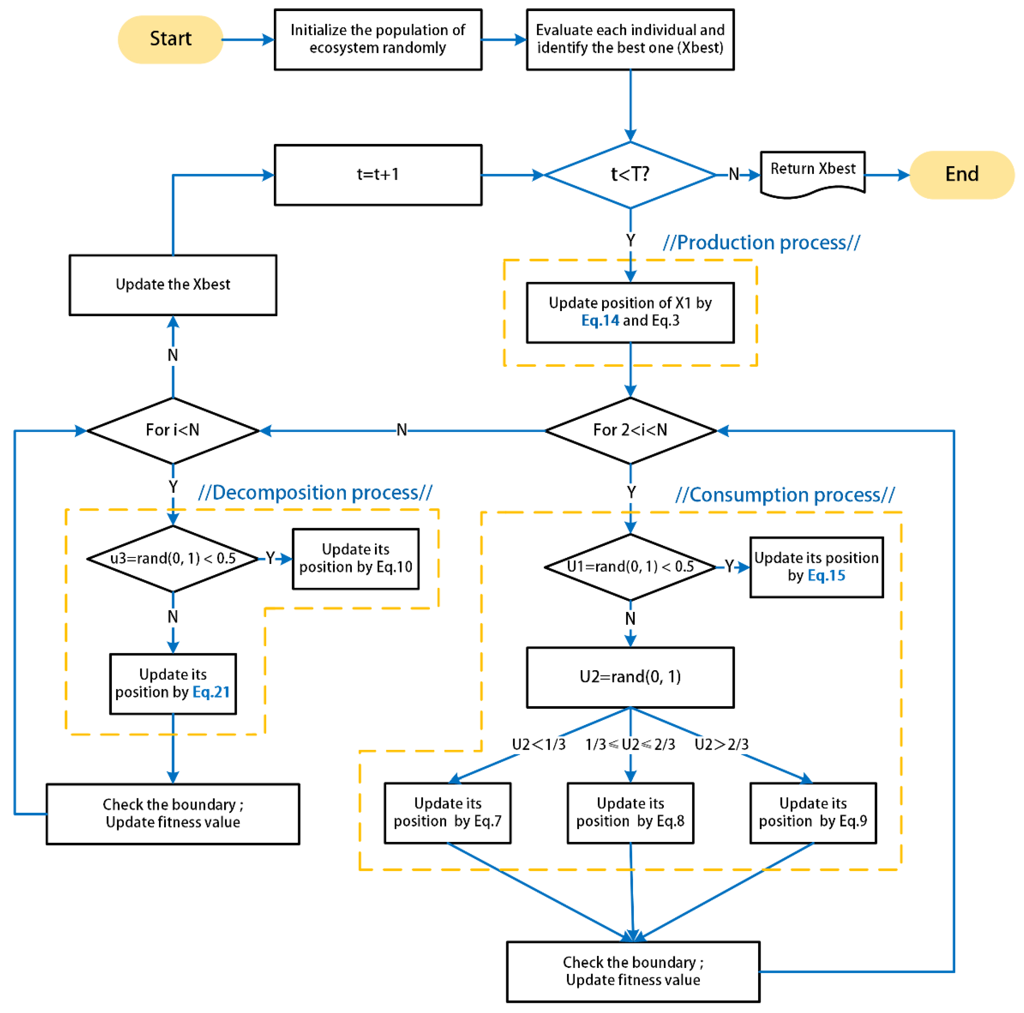
The Artificial Ecosystem Optimization (AEO) algorithm created by Zhao et al. [23] is a metaheuristic optimization algorithm based on the principles of ecosystem energy dynamics. This algorithm represents a model based on three stages, namely, production, consumption, and decomposition. The populations in the model include producers representing the worst solution, decomposers representing the optimal solution, and multilevel consumers ranked by fitness, among which consumers simulate the herbivores, carnivores, and omnivores in the food chain depending on their fitness.
Production stage: In the production stage, the worst individual (producer) is updated based on the upper and lower bounds information in the search space and the characteristics of the best individual (decomposer), the step control parameter is adjusted through linear decrease to achieve search balance, and a new individual with higher exploration potential is generated. This process can be mathematically expressed as:
where is the maximum number of iterations, is a random number within the range of [0, 1], is a coefficient used for linear weighting, is the population size, is a random vector within the range of [0, 1], is the upper bound, and is the lower bound.
Consumption stage: In the consumption stage, consumers obtain “nutrition” from other organisms based on their position in the food chain to improve the solution. In order to avoid complexity in parameter adjustment, a simple, parameter-free random walk strategy with the characteristics of Levy flight is proposed, which is called the consumption factor C. In this stage, different types of consumers are updated according to different rules. Specifically, herbivores are updated according to Equation (7), carnivores are updated according to Equation (8), and omnivores are updated according to Equation (9).
where denotes uniformly distributed random numbers between 0 and 1.
Decomposition stage: This stage is similar to the process of decomposition of biological remains by decomposers in an ecosystem, and its purpose is to enhance the exploration and exploitation of the neighborhood of the optimal solution. This process can be mathematically expressed as:
2.3.3. SAEO Algorithm
In this paper, an improved metaheuristic algorithm based on the AEO algorithm, which is called the SAEO algorithm, is proposed to improve the performance of the original AEO algorithm.
Production stage: The original AEO algorithm adjusts the step control parameter α through linear decrement during the production phase to achieve search balance. However, this method has limitations when simulating complex nonlinear ecological evolution [32]. The SAEO algorithm addresses this limitation by introducing a nonlinear function to dynamically update the α value during the development phase. This optimization strategy aims to enhance the algorithm’s ability to solve nonlinear problems.
Consumption stage: The original AEO algorithm adopts a simple, parameter-less random walk strategy, which lacks flexibility when dealing with complex problems. The SAEO algorithm addresses this limitation by optimizing it. During each iteration, each individual has a 50% chance of evolving according to the basic AEO algorithm. Simultaneously, there is a 50% chance of incorporating global exploration using Levy flight trajectories based on Equation (15) [33]. This optimization strategy aims to enhance the algorithm’s global exploration capability.
where is generated based on the Levy distribution, and the parameter β of this distribution is randomly selected in the range of [0, 2] [34,35]. The related mathematical formulas are given below.
Decomposition stage: The original AEO algorithm employs a single strategy for evolutionary operations, which may lead to overfitting risks. The SAEO algorithm optimizes this by introducing a dynamic crossover strategy. During each iteration, each individual has a 50% chance of evolving according to the basic AEO algorithm, and there is a 50% chance of adopting the dynamic crossover strategy. This strategy involves randomly selecting an individual, , from the entire population and updating it according to Equation (21). This optimization strategy aims to ensure that the population can continuously optimize and move towards the global optimal state throughout the iterations.
The operation process of the SAEO algorithm is shown in Figure 2.
2.3.4. Building of the SAEO-BP Neural Network Model
In this study, the Chl-a concentration prediction model was trained using the SAEO algorithm in combination with a BP neural network. The complete process of this model consists of three major links, namely, data preprocessing, model building, and model performance evaluation (Figure 3).
In the data preprocessing stage, a total of 612 valid data records were obtained and divided into a training set and a test set. The training set was used for model building and training, and the test set was used for model evaluation.
In the model building stage, the spectral values of 12 bands in the training set were used as input features, and the SAEO-BP neural network was used to train the Chl-a concentration prediction model. Specifically, the weights and biases in the network were set as decision variables of the optimization problem, and the mean squared error (MSE) for the objective function was set. Subsequently, the SAEO algorithm was used to iteratively optimize these parameters until the preset maximum number of iterations was reached. When the optimal solution was produced, the optimal parameter vector was extracted and used to train the BP neural network. After training was completed, it was applied on the test set to evaluate the performance of the SAEO-BP neural network.
In the model evaluation stage, the trained SAEO-BP neural network was quantitatively evaluated using a series of performance indicators widely used in the field of remote sensing, including the coefficient of determination (R2), mean squared error (MSE), mean absolute error (MAE), and root mean squared error (RMSE). The mathematical expressions of these indicators are given below.
where is the predicted value of Chl-a concentration, is the actual (measured) value of Chl-a concentration, is the average of all measured values of Chl-a concentration, and N is the total sample size.
Finally, the Chl-a concentration prediction model was applied on the Sentinel-2 satellite imagery data selected for a particular period, including the data of heavy precipitation events and red tides, to produce spatial distribution maps for Chl-a concentration in the experimental areas. The spatial and temporal variations in Chl-a concentration during particular events were visually analyzed to demonstrate the model’s actual performance in application scenarios and its capability to monitor environmental changes.
3. Results
First, the performance of the SAEO-BP neural network model was evaluated. Subsequently, the model was applied in scenarios involving large fluctuations in Chl-a concentration resulting from heavy precipitation events and red tides, the patterns of spatiotemporal variation in Chl-a concentration in the coastal waters of Hong Kong were identified through inversion, and the model’s prediction accuracy in scenarios involving dramatic changes was verified.
3.1. Model Performance Evaluation
This section focuses on investigating the performance of the SAEO-BP neural network in predicting Chl-a concentration. First, an ablation experiment was conducted to determine the performance of the optimization scheme. Then, the performance of the SAEO-BP neural network was compared with that of the BP neural network optimized using the AEO algorithm (AEO-BP neural network). Finally, 16 representative metaheuristic optimization algorithms were selected for comparison, and the performance of different neural network models in Chl-a concentration prediction was comparatively analyzed in an in-depth manner.
During the experiment, all metaheuristic optimization algorithms to be compared were programmed and implemented using the open source Python library MEALPY 2.4.1 [36] to ensure the consistent execution of different optimization strategies and effective comparison of the results produced.
3.1.1. Ablation Experiment
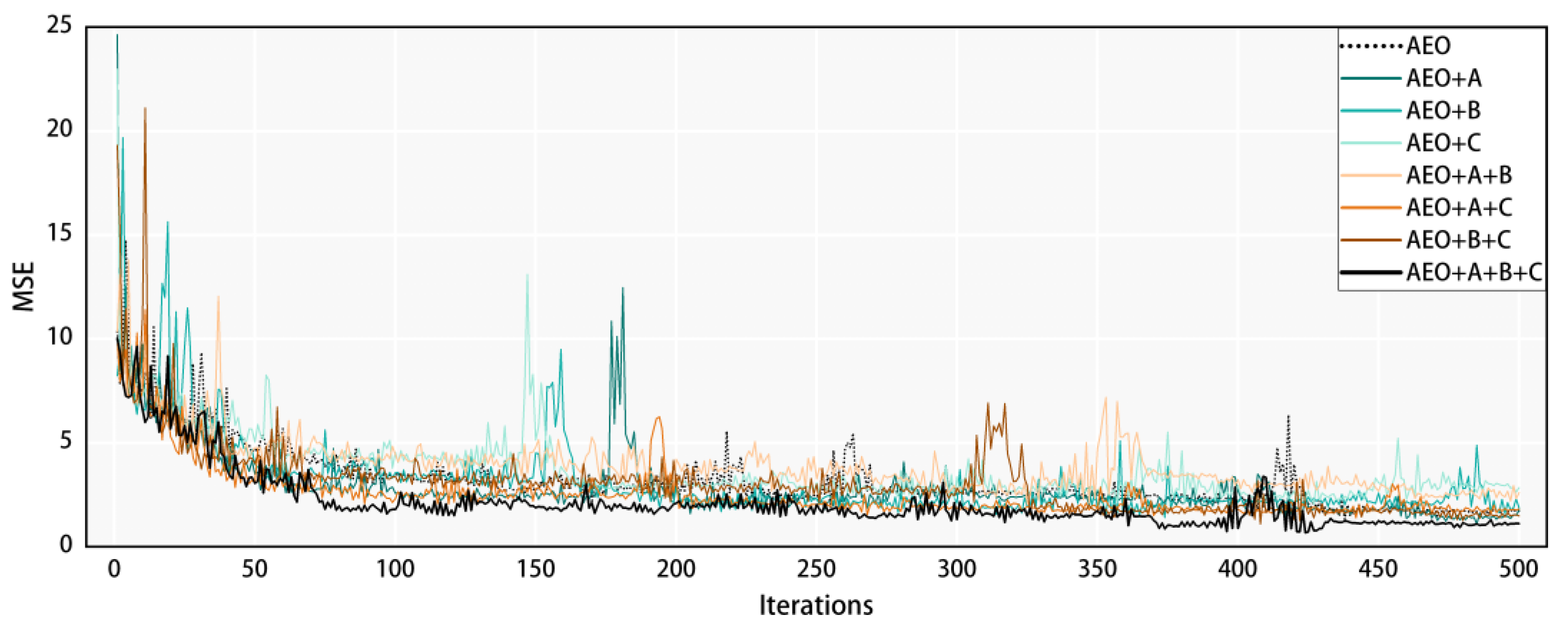
An ablation experiment was conducted to investigate the feasibility of the AEO algorithm-based optimization scheme and demonstrate the specific meaning of each module. Figure 4 shows the training losses of the BP neural networks optimized using different metaheuristic optimization algorithms, including the original AEO algorithm and AEO algorithms incorporating one or more of the nonlinear weight coefficient, the “Levy flight path” search strategy, and the dynamic crossover mechanism. The experiment showed that when these mechanisms were, respectively, integrated with three algorithms, the balance between global exploration and local exploitation was affected, resulting in training loss fluctuations, slower convergence, and poor convergence performance. When two of these mechanisms were incorporated into one algorithm, the optimization performance was not stable; when these three mechanisms were integrated with the same algorithm, the model’s convergence performance tended to become stable, and its training loss was significantly reduced. These results show that each of the three mechanisms plays an important role in optimizing the AEO algorithm.
3.1.2. Comparative Analysis of the Performance of the SAEO-BP and AEO-BP Neural Networks
In this study, the performance of the SAEO-BP and AEO-BP neural networks was evaluated using the following four indicators: R2, MSE, MAE, and RMSE. All models were trained for 10 times with the same settings (epoch = 500, pop_size = 50), and the average values of all indicators was recorded (Table 2). The experimental results show that the SAEO-BP neural network performs better than the AEO-BP neural network in the training process, and the superior performance of the former is reflected in higher R2 (0.9214) and lower MSE (1.1201), MAE (0.2774) and RMSE (1.0581). This indicates that the SAEO-BP neural network can better describe the data set and produces smaller prediction errors in the learning process. For the testing process, the R2 value of the SAEO-BP neural network is 0.7307, which is greater than that of the AEO-BP neural network (0.6828), and the SAEO-BP neural network has the lowest values of MSE, MAE and RMSE, which clearly demonstrates its high prediction accuracy. Figure 5 depicts a line graph of the validation dataset, which includes both the measured values of Chl-a concentration and the predicted values obtained using two models. It is observed that compared to the AEO-BP neural network model, the predictions of the SAEO-BP neural network model exhibit higher overall consistency with the measured values. The SAEO-BP model provides more accurate descriptions of both extreme values and minor fluctuations, enabling it to predict short-term rapid changes in Chl-a concentration more effectively.
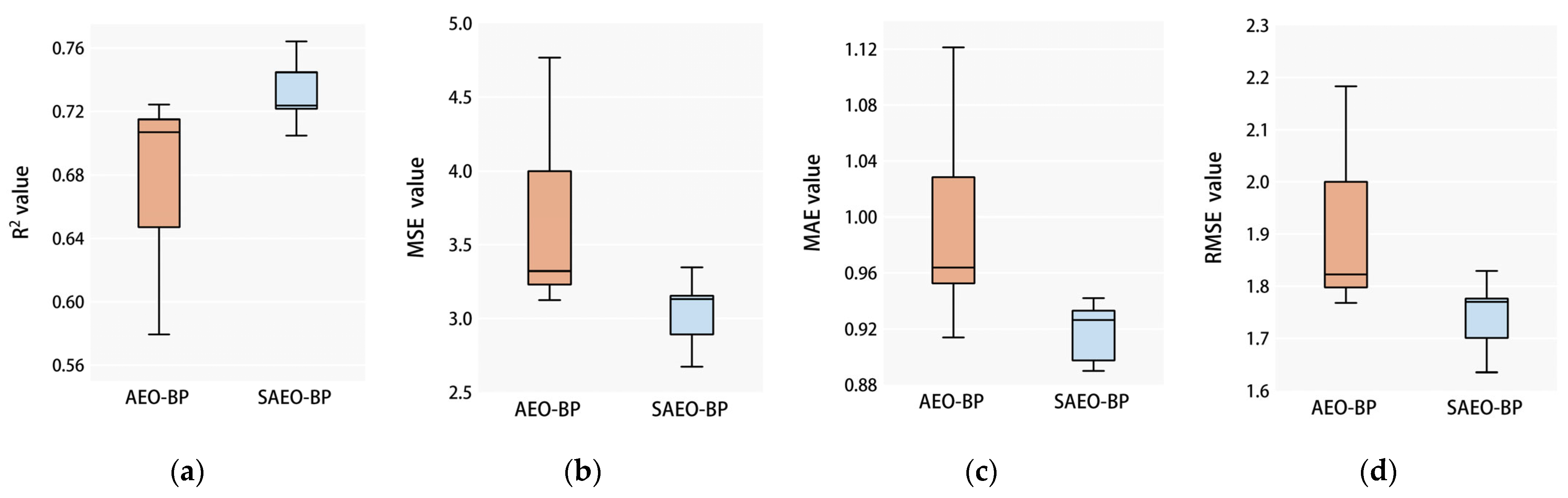
In addition, the results from 10 occasions of training were visually presented in box plots and compared (Figure 6). The comparison results show that the SAEO-BP neural network performs more stably than the AEO-BP neural network.
3.1.3. Comparative Analysis of the Performance of the SAEO-BP Neural Network and Other BP Neural Networks Based on Metaheuristic Optimization Algorithms
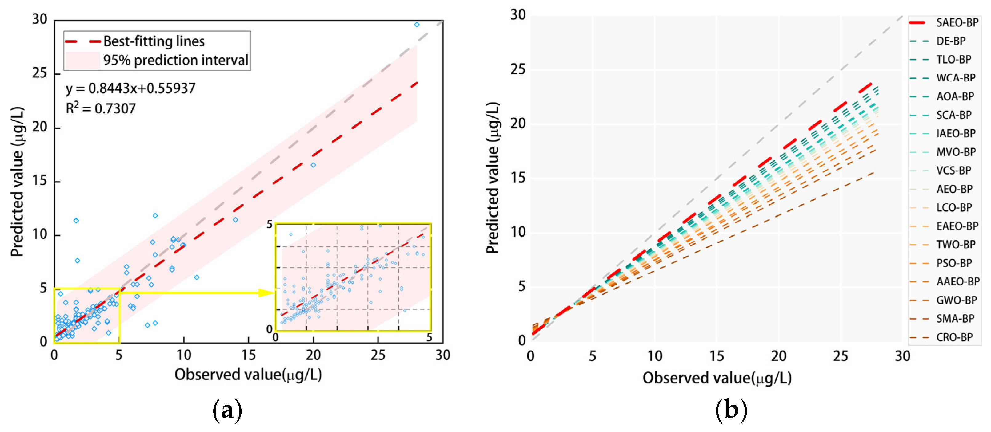
Other BP neural network models optimized using 16 metaheuristic optimization algorithms were used to predict Chl-a concentration. All models were trained for 10 times with the same settings (epoch = 500, pop_size = 50), and the average values of all indicators was recorded. The results in Table 3 show that the SAEO-BP neural network has advantages in the training set, and these advantages are further enhanced in the validation set. The SAEO-BP neural network has achieved the best results in terms of R2 (0.7307), MSE (3.0521), MAE (0.9185), and RMSE (1.746). Figure 7 illustrates the distribution of validation set data after training with the SAEO-BP neural network, along with the fitting lines of validation set data after training with 17 other algorithms, providing visual evidence of the superiority of the SAEO-BP neural network in predicting Chl-a concentration.
The stability of different models was comparatively analyzed in an all-round way using box plots showing the results of 17 models trained on the test set for 10 times (Figure 8). The results show that, in terms of MAE, the SAEO-BP neural network has the highest stability, followed by the IAEO-BP and VCS-BP neural networks; in terms of the other three performance indicators, the SAEO-BP has a high stability, second only to the IAEO-BP neural network.
In summary, the SAEO-BP neural network proposed in this paper performs better than the BP neural networks optimized using other metaheuristic optimization algorithms in terms of prediction accuracy and stability, providing a good solution to predicting Chl-a concentration under complex environmental conditions.
3.2. Investigation of the Inversion Performance of the SAEO-BP Neural Network under Conditions of Significant Changes in Chl-a Concentration
As mentioned earlier, the SAEO-BP neural network model established based on historical data performed well during the evaluation phase. To assess whether the model can accurately predict short-term drastic changes in chlorophyll-a concentration caused by extreme events, this study evaluates the model’s prediction results for extreme low values during heavy rainfall periods and extremely high values during red tide outbreaks in the study area. Specifically, predictions were made for the Chl-a concentration during heavy rainfall periods in regions A, B, and C from 6 October 6 to 10 November 2021, as well as during the red tide outbreak period in region D from 8 March to 23 March 2021. By comparing the model’s predicted values with the actual scenarios, and assessing the consistency between the maximum and minimum values at the same observation location on different days within the experimental period, the paper aims to determine the model’s predictive accuracy.
3.2.1. Analysis of the Accuracy of the SAEO-BP Neural Network and Its Sensitivity to Spatial and Temporal Changes in Chl-a Concentration during Extreme Precipitation Events
According to the research findings of Zhou et al. [25], Chl-a concentration will decrease during typhoons, but in a few days after a typhoon, new conditions favorable for algae growth will be established and Chl-a concentration will increase. In order to verify the sensitivity of the SAEO-BP neural network to the spatial and temporal (dynamic) changes in Chl-a concentration, the remote sensing images for the period in which Hong Kong was affected by tropical cyclones Lionrock and Kompasu (October 2021) were selected for inversion and analysis, with the focus on the spatial and temporal changes in Chl-a concentration in experimental Areas A, B, and C.
In October 2021, affected by the two typhoons mentioned above, the cumulative precipitation in Hong Kong during this period increased significantly and reached 631.1 mm, which is more than five times the average precipitation for the same period in history. According to the climate data provided by the Hong Kong Observatory, after Lionrock made landfall on 7 October 2021, Hong Kong experienced continued heavy rainfall; as the typhoon moved away on 11 October 2021, the precipitation decreased, and the weather cleared up. Kompasu approached Hong Kong on 12 October 2021, resulting in widespread precipitation, and the weather gradually cleared up on 16 October 2021.
Based on these changes in precipitation, two groups of key points in time were selected. The time points in the first group are 6, 11 and 16 October 2021, which were selected to reveal the changes in Chl-a concentration within the study area on the day before the onset of heavy precipitation, during heavy precipitation, and on the day when heavy precipitation ended. The time point in the second group is 10 November 2021, which was selected to observe the changes in Chl-a concentration within a certain period of time after heavy precipitation ended. Since the cumulative precipitation in the period from 16 October to 10 November 2021 is less than 10 mm, its impact on Chl-a concentration in the study area can be ignored.
The study employed the trained SAEO-BP neural network model to retrieve the Chl-a concentration from images taken on different dates in each experimental area (Figure 9). Table 4 lists the mean Chl-a concentration obtained through inversion from each image and the records of the cumulative precipitation in Hong Kong for several five-day periods are given in Table 5. The tabulated data show that the cumulative precipitation in the first five-day period before the onset of heavy precipitation (from 2 October to 6 October 2021) is only 1.9 mm and the average values of Chl-a concentration in the three experimental areas are at levels higher than 7 μg/L. The cumulative precipitation in the five-day period of the first heavy rainfall event (from 7 October to 11 October 2021) reached 549 mm, resulting in abrupt decreases in the average Chl-a concentration in the three experimental areas. The inversion results for 11 October 2021 show that the average Chl-a concentration is 3.90 μg/L in experimental Area A, 3.12 μg/L in experimental Area B, and 1.38 μg/L in experimental Area C. Subsequently, the second heavy rainfall event occurred from 12 October to 16 October 2021, resulting in cumulative precipitation of 75.8 mm in five days and the average values of Chl-a concentration in the three experimental areas decreased again. The average Chl-a concentration as of 16 October 2021 is 3.08 μg/L in experimental Area A, 1.93 μg/L in experimental Area B, and 1.22 μg/L in experimental Area C. As the second heavy rainfall event ended, the Chl-a concentration in the coastal waters began to increase. The average Chl-a concentration as of 10 November 2021 is 4.81 μg/L in experimental Area A, 4.73 μg/L in experimental Area B, and 3.16 μg/L in experimental Area C. These results are consistent with the monitoring results (https://khoyinivan.users.earthengine.app/view/marine-water-quality-hk, accessed on 15 January 2024) [22] and demonstrate that the SAEO-BP neural network model can effectively capture large fluctuations/changes in Chl-a concentration under heavy precipitation conditions.
3.2.2. Simulation of Changes in Chl-a Concentration during Red Tides and Its Spatial Distribution Characteristics Using the SAEO-BP Neural Network Model
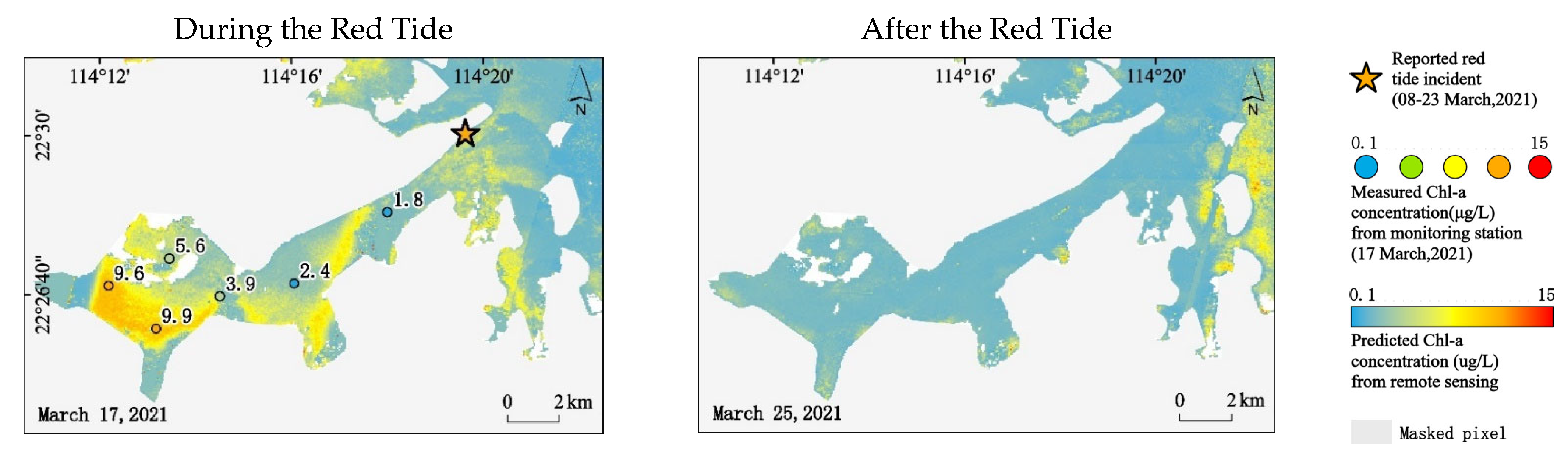
In addition, the effectiveness and stability of the SAEO-BP neural network model under complex environmental conditions were further verified by comparing the data acquired during red tides; this study further confirmed the effectiveness and stability of the SAEO-BP neural network model under complex environmental conditions. According to information from the Hong Kong Red Tide Database (https://redtide.afcd.gov.hk/urtin/#/maps, accessed on 15 January 2024), a continuous red tide caused by Gonyaulax polygramma occurred in the Tolo Channel northeast of Hong Kong during the period from 8 March to 23 March 2021.
Chl-a concentration is usually used to represent phytoplankton biomass. In this study, the SAEO-BP neural network model was used to perform the inversion of Chl-a concentration in experimental Area D, and the Chl-a concentration distribution in this area on 17 March and 25 March 2021 was visually displayed (Figure 10) to demonstrate the spatial variations in Chl-a concentration during and after the red tide.
It can be seen that the Chl-a concentration map for 17 March 2021 has accurately captured the distribution characteristics (high levels) of Chl-a concentration in the Tolo Channel on that day, and the predicted values of Chl-a concentration in the surrounding areas are basically consistent with the measured data from the monitoring station on that day. The Chl-a concentration map for 25 March 2021 shows the distribution of Chl-a concentration in the Tolo Channel and surrounding areas after the red tide dissipated. It can be seen that the Chl-a concentration in the Tolo Channel decreased significantly on 25 March 2021. These results show that the SAEO-BP neural network model can effectively reflect water conditions during red tides.
4. Discussion
In this section, we first introduce the results of optimizing the BP neural network using the SAEO algorithm. Secondly, we describe the effectiveness of the Chl-a inversion model constructed using the SAEO-BP neural network model, confirming the advantages of the SAEO-BP neural network model in prediction accuracy and stability. Finally, by comparing it with traditional regression algorithms, simplified physical model algorithms (QAA), and commonly used machine learning algorithms (SVR), we verify the effectiveness of the SAEO algorithm in optimizing the BP neural network model.
4.1. Performance of the SAEO Algorithm in Optimizing BP Neural Networks
In the AEO algorithm, producers are mainly responsible for exploring new possible solutions, consumers further explore the solution space through three mechanisms, and decomposers improve the exploration efficiency by referring to existing solutions. Such configuration enables the AEO algorithm to further expand the scope of search for solutions while maintaining efficient exploration. On this basis, the nonlinear weight coefficient, the “Levy flight” path search strategy, and the dynamic crossover mechanism were incorporated into the AEO algorithm to further improve its performance in optimizing BP neural networks, and an ablation experiment was conducted. The results show that the incorporation of these three mechanisms can effectively balance global exploration and local exploitation, stabilize the loss in the training process (training loss), and thereby improve the convergence rate and performance.
The SAEO algorithm was compared with other 17 metaheuristic optimization algorithms to verify its performance in optimizing BP neural networks. The results show that the BP neural network optimized using the improved AEO algorithm has advantages in terms of prediction accuracy and stability. In addition, these results demonstrate the powerful performance of the original AEO algorithm and prove that the SAEO algorithm can effectively overcome the limitations of BP neural networks, such as their tendency to become stuck in local optima and large fluctuations in accuracy.
4.2. Performance of the Chl-a Concentration Inversion Model Built Based on the SAEO-BP Neural Network
In water environment research, water quality monitoring plays a vital role, and Chl-a concentration is widely recognized as a key measure of water quality. In this study, an innovative optimization algorithm based on the AEO algorithm, namely the SAEO algorithm, was proposed and used to optimize the BP neural network to improve the accuracy of Chl-a concentration prediction. The SAEO-BP neural network model for predicting Chl-a concentration in the coastal waters of Hong Kong was built. The results of comparison and verification show that the SAEO-BP neural network model is more accurate and stable than the neural networks optimized using the AEO algorithm and other metaheuristic optimization algorithms.
By inverting and analyzing the remote sensing data of Hong Kong waters for the period in which Hong Kong was affected by Lionrock and Kompasu (October 2021), previous theories on the impact of typhoons on marine ecosystems were verified. Specifically, heavy precipitation and wind caused drastic changes in the water environment of the study area, significantly enhanced vertical mixing, accelerated the dilution process, and increased the water exchange rate, resulting in rapid short-term (for the period from 6 October to 11 October 2021 and the period from 12 October to 16 October 2021) decreases in Chl-a concentration from high levels (above 7 μg/L) to around 3 μg/L or even lower levels. After typhoons ended, with the decrease in precipitation and the weakening of vertical mixing, a large amount of Pearl River water (runoff) rich in nitrogen-containing nutrient salts flew into the ocean, providing favorable conditions for algae reproduction. Therefore, for a certain period of time (such as 10 November 2021), the average levels of Chl-a concentration in various monitored coastal areas of Hong Kong rose to 4.81 μg/L, 4.73 μg/L, and 3.16 μg/L, respectively.
In addition, a red tide that occurred in the Tolo Channel northeast of Hong Kong in the period from 8 March to 23 March 2021 was investigated. The results of the inversion of remote sensing images show that the Chl-a concentration in the Tolo Channel increased abruptly on 17 March 2021, which is consistent with the occurrence of the red tide in this area, and on 25 March 2021, the Chl-a concentration near the Tolo Channel decreased to a normal level, which is consistent with the reported dissipation of the red tide. These results further verify the accuracy of the SAEO-BP neural network model in predicting Chl-a concentration during the occurrence and dissipation of red tides.
4.3. Validation of the Effectiveness of SAEO Algorithm Optimized BP Neural Network Model
In research related to the inversion of water quality parameters in small samples, traditional algorithmic models are simple to establish and computationally fast, but their accuracy is relatively low. Physical methods have clear mechanisms, but the models are overly complex, requiring numerous parameters, and exhibit unstable prediction accuracy across different water bodies. Machine learning algorithms are suitable for solving nonlinear problems, but finding the optimal parameter settings for the model is challenging, although their accuracy is relatively higher compared to the first two types of algorithms. This paper compares the proposed SAEO-BP neural network model with empirical algorithms, commonly used simplified physical model algorithms (QAA [47]), and the Support Vector Regression (SVR) algorithm (Figure 11), which is widely used in machine learning algorithms, to verify the effectiveness of the SAEO algorithm in optimizing the BP neural network model for data prediction.
In the experiment, the model trained with the training dataset will be applied to the dataset covering all samples. By comparing the distribution of predicted values with actual measurements and plotting fitting curves, the study found significant differences between the predicted values calculated using the linear regression algorithm and QAA algorithm and the actual measurements, indicating a lower accuracy of the algorithms. Machine learning algorithms demonstrated superiority in predicting accuracy, especially the model based on SAEO-BP neural network, which showed the best predictive performance and significantly outperformed the other three methods, validating the effectiveness of the SAEO-BP neural network algorithm in data prediction.
5. Conclusions
In order to improve the accuracy and stability of the Chl-a concentration prediction model, 5754 valid observation records of Chl-a concentration in the coastal waters of Hong Kong for the period from 2017 to 2022 and 500 high-quality Sentinel-2 remote sensing images for the same period were collected, and 612 pieces of valid data were selected and used for model training and validation. Based on this data set, the levels of Chl-a concentration in the coastal waters of Hong Kong were predicted and analyzed through inversion. The main achievements of this study are summarized below.
- Algorithm innovation and model building: An improved metaheuristic optimization algorithm, namely, the Synthesized Artificial Ecosystem Optimization (SAEO) algorithm, was proposed. First, the algorithm was integrated with the adaptive nonlinear weight coefficient, the “Levy flight” path search strategy, and the dynamic crossover mechanism to overcome its limitations in solving complex problems and to enhance its global search capability. Then, a novel model named the SAEO-BP neural network model was built by combining the SAEO algorithm with a BP neural network and was used for Chl-a concentration prediction.
- Performance evaluation and comparative analysis: The experimental results show that, compared with the AEO-BP neural network model, the SAEO-BP neural network model produced smaller prediction errors in the training and testing stages and performed more stably in the testing stage. In addition, the SAEO-BP neural network model has obvious advantages over 16 BP neural networks optimized using different metaheuristic optimization algorithms in terms of all key performance indicators. The comparative analysis of the stability of these models shows that the SAEO-BP neural network model has the highest stability in terms of MAE and is highly stable in terms of the other three indicators.
- Prediction and evaluation of abrupt changes in Chl-a concentration: The SAEO-BP neural network model was used to identify the patterns of spatiotemporal variation in Chl-a concentration in the coastal waters of Hong Kong during heavy precipitation events and red tides. The results show that the SAEO-BP neural network model can predict the spatiotemporal changes in Chl-a concentration under the influence of heavy precipitation caused by typhoons, identify the spatial variations in Chl-a concentration during and after red tides, and predict abrupt Chl-a concentration changes and extrema in an accurate and stable manner.
There are still some shortcomings in this study. The Chl-a concentration inversion model built using Sentinel-2 remote sensing data still has some inherent limitations. The discontinuity of satellite revisit cycles and cloud cover pose obstacles to obtaining continuous and high-quality remote sensing data. Moreover, although Sentinel-2 satellite remote sensing imagery data provide a rich information basis for Chl-a inversion, the generalizability of algorithms to other marine areas under different geographical conditions, lighting conditions, water characteristics, and other environmental variables still needs to be considered.
Future research should focus on integrating multi-source remote sensing data resources, optimizing atmospheric correction algorithms, and improving the quantity and quality of remote sensing data applicable to coastal water quality monitoring. Additionally, combining field sampling data, considering key water quality parameters such as suspended sediment and nutrient concentration that affect the optical properties of water bodies, thoroughly analyzing the complex relationships between water quality parameters, constructing coupled models, and more accurately describing the water quality status and variation characteristics of coastal waters will provide a more reliable data source for water environment monitoring and management.
Author Contributions
Conceptualization, X.W. and J.C.; methodology, X.W.; software, X.W.; validation, X.W.; formal analysis, X.W. and J.C.; investigation, X.W.; resources, J.C. and M.X.; data curation, X.W.; writing—original draft preparation, X.W.; writing—review and editing, X.W.; visualization, X.W.; supervision, J.C. and M.X.; project administration, X.W. All authors have read and agreed to the published version of the manuscript.
Funding
This research was funded by the National Natural Science Foundation of China under Grant U1906217, 62071491 and the Fundamental Research Funds for the Central Universities 22CX01004A-5, 22CX01004A-4.
Data Availability Statement
The measured water quality data are available from HKEPD (https://www.epd.gov.hk/epd/sc_chi/environmentinhk/water/hkwqrc/waterquality/marine.html) (accessed on 1 August 2023). The surface reflectance datasets of Sentinel-2 are available on GEE (https://earthengine.google.com) (accessed on 1 August 2023). The precipitation data are available from the Hong Kong Observatory. (https://www.weather.gov.hk/tc/wxinfo/pastwx/mws/mws.htm) (accessed on 15 January 2024). Hong Kong red tide data can be obtained through the following link (https://redtide.afcd.gov.hk/urtin/#/maps) (accessed on 15 January 2024).
Acknowledgments
We thank the developers for their tools and the respective agencies that provided the data. We further thank all editors and anonymous reviewers for spending their time working on the manuscript.
Conflicts of Interest
The authors declare no conflicts of interest.
References
- Gholizadeh, M.H.; Melesse, A.M.; Reddi, L. A Comprehensive Review on Water Quality Parameters Estimation Using Remote Sensing Techniques. Sensors 2016, 16, 1298. [Google Scholar] [CrossRef]
- Poddar, S.; Chacko, N.; Swain, D. Estimation of Chlorophyll-a in Northern Coastal Bay of Bengal Using Landsat-8 OLI and Sentinel-2 MSI Sensors. Front. Mar. Sci. 2019, 6, 598. [Google Scholar] [CrossRef]
- Flores-Anderson, A.I.; Griffin, R.; Dix, M.; Romero-Oliva, C.S.; Ochaeta, G.; Skinner-Alvarado, J.; Ramirez Moran, M.V.; Hernandez, B.; Cherrington, E.; Page, B.; et al. Hyperspectral Satellite Remote Sensing of Water Quality in Lake Atitlán, Guatemala. Front. Environ. Sci. 2020, 8, 7. [Google Scholar] [CrossRef]
- Pizani, F.M.C.; Maillard, P.; Ferreira, A.F.F.; de Amorim, C.C. Estimation of water quality in a reservoir from Sentinel-2 MSI and Landsat-8 OLI sensors. ISPRS Ann. Photogramm. Remote Sens. Spat. Inf. Sci. 2020, 3, 401–408. [Google Scholar] [CrossRef]
- Chen, J.; Chen, S.; Fu, R.; Li, D.; Jiang, H.; Wang, C.; Peng, Y.; Jia, K.; Hicks, B.J. Remote Sensing Big Data for Water Environment Monitoring: Current Status, Challenges, and Future Prospects. Earth’s Future 2022, 10, e2021EF002289. [Google Scholar] [CrossRef]
- Wang, X.; Yang, W. Water Quality Monitoring and Evaluation Using Remote Sensing Techniques in China: A Systematic Review. Ecosyst. Health Sustain. 2019, 5, 47–56. [Google Scholar] [CrossRef]
- Sobel, R.S.; Kiaghadi, A.; Rifai, H.S. Modeling Water Quality Impacts from Hurricanes and Extreme Weather Events in Urban Coastal Systems Using Sentinel-2 Spectral Data. Environ. Monit. Assess. 2020, 192, 307. [Google Scholar] [CrossRef]
- Gitelson, A.A.; Dall’Olmo, G.; Moses, W.; Rundquist, D.C.; Barrow, T.; Fisher, T.R.; Gurlin, D.; Holz, J. A Simple Semi-Analytical Model for Remote Estimation of Chlorophyll-a in Turbid Waters: Validation. Remote Sens. Environ. 2008, 112, 3582–3593. [Google Scholar] [CrossRef]
- Yang, Y.; Zhang, X.; Gao, W.; Zhang, Y.; Hou, X. Improving Lake Chlorophyll-a Interpreting Accuracy by Combining Spectral and Texture Features of Remote Sensing. Environ. Sci. Pollut. Res. 2023, 30, 83628–83642. [Google Scholar] [CrossRef] [PubMed]
- O’Reilly, J.E.; Werdell, P.J. Chlorophyll Algorithms for Ocean Color Sensors—OC4, OC5 & OC6. Remote Sens. Environ. 2019, 229, 32–47. [Google Scholar] [CrossRef]
- Hu, C.; Feng, L.; Lee, Z.; Franz, B.A.; Bailey, S.W.; Werdell, P.J.; Proctor, C.W. Improving Satellite Global Chlorophyll a Data Products Through Algorithm Refinement and Data Recovery. J. Geophys. Res. Ocean. 2019, 124, 1524–1543. [Google Scholar] [CrossRef]
- Rodríguez-López, L.; Duran-Llacer, I.; González-Rodríguez, L.; Abarca-del-Rio, R.; Cárdenas, R.; Parra, O.; Martínez-Retureta, R.; Urrutia, R. Spectral Analysis Using LANDSAT Images to Monitor the Chlorophyll-a Concentration in Lake Laja in Chile. Ecol. Inform. 2020, 60, 101183. [Google Scholar] [CrossRef]
- Hafeez, S.; Wong, M.S.; Ho, H.C.; Nazeer, M.; Nichol, J.; Abbas, S.; Tang, D.; Lee, K.H.; Pun, L. Comparison of Machine Learning Algorithms for Retrieval of Water Quality Indicators in Case-II Waters: A Case Study of Hong Kong. Remote Sens. 2019, 11, 617. [Google Scholar] [CrossRef]
- Kwong, I.H.Y.; Wong, F.K.K.; Fung, T. Automatic Mapping and Monitoring of Marine Water Quality Parameters in Hong Kong Using Sentinel-2 Image Time-Series and Google Earth Engine Cloud Computing. Front. Mar. Sci. 2022, 9, 871470. [Google Scholar] [CrossRef]
- Zhu, W.-D.; Qian, C.-Y.; He, N.-Y.; Kong, Y.-X.; Zou, Z.-Y.; Li, Y.-W. Research on Chlorophyll-a Concentration Retrieval Based on BP Neural Network Model-Case Study of Dianshan Lake, China. Sustainability 2022, 14, 8894. [Google Scholar] [CrossRef]
- Jiang, B.; Liu, H.; Xing, Q.; Cai, J.; Zheng, X.; Li, L.; Liu, S.; Zheng, Z.; Xu, H.; Meng, L. Evaluating Traditional Empirical Models and BPNN Models in Monitoring the Concentrations of Chlorophyll-A and Total Suspended Particulate of Eutrophic and Turbid Waters. Water 2021, 13, 650. [Google Scholar] [CrossRef]
- Li, Z.; Zhao, X. BP Artificial Neural Network Based Wave Front Correction for Sensor-Less Free Space Optics Communication. Opt. Commun. 2017, 385, 219–228. [Google Scholar] [CrossRef]
- Zheng, B.-H. Material Procedure Quality Forecast Based on Genetic BP Neural Network. Mod. Phys. Lett. B 2017, 31, 1740080. [Google Scholar] [CrossRef]
- Pyo, J.; Duan, H.; Ligaray, M.; Kim, M.; Baek, S.; Kwon, Y.S.; Lee, H.; Kang, T.; Kim, K.; Cha, Y.; et al. An Integrative Remote Sensing Application of Stacked Autoencoder for Atmospheric Correction and Cyanobacteria Estimation Using Hyperspectral Imagery. Remote Sens. 2020, 12, 1073. [Google Scholar] [CrossRef]
- Deng, Y.; Xiao, H.; Xu, J.; Wang, H. Prediction Model of PSO-BP Neural Network on Coliform Amount in Special Food. Saudi J. Biol. Sci. 2019, 26, 1154–1160. [Google Scholar] [CrossRef]
- Zhu, C.; Zhang, J.; Liu, Y.; Ma, D.; Li, M.; Xiang, B. Comparison of GA-BP and PSO-BP Neural Network Models with Initial BP Model for Rainfall-Induced Landslides Risk Assessment in Regional Scale: A Case Study in Sichuan, China. Nat. Hazards 2020, 100, 173–204. [Google Scholar] [CrossRef]
- Huang, Y.; Xiang, Y.; Zhao, R.; Cheng, Z. Air Quality Prediction Using Improved PSO-BP Neural Network. IEEE Access 2020, 8, 99346–99353. [Google Scholar] [CrossRef]
- Zhao, W.; Wang, L.; Zhang, Z. Artificial Ecosystem-Based Optimization: A Novel Nature-Inspired Meta-Heuristic Algorithm. Neural Comput. Appl. 2020, 32, 9383–9425. [Google Scholar] [CrossRef]
- Li, J.; Peng, B.; Wei, Y.; Ye, H. Accurate Extraction of Surface Water in Complex Environment Based on Google Earth Engine and Sentinel-2. PLoS ONE 2021, 16, e0253209. [Google Scholar] [CrossRef]
- Zhou, W.; Yin, K.; Harrison, P.J.; Lee, J.H.W. The Influence of Late Summer Typhoons and High River Discharge on Water Quality in Hong Kong Waters. Estuar. Coast. Shelf Sci. 2012, 111, 35–47. [Google Scholar] [CrossRef]
- Xu, J.; Yin, K.; Lee, J.H.W.; Liu, H.; Ho, A.Y.T.; Yuan, X.; Harrison, P.J. Long-Term and Seasonal Changes in Nutrients, Phytoplankton Biomass, and Dissolved Oxygen in Deep Bay, Hong Kong. Estuaries Coasts 2010, 33, 399–416. [Google Scholar] [CrossRef]
- Deng, T.; Duan, H.-F.; Keramat, A. Spatiotemporal Characterization and Forecasting of Coastal Water Quality in the Semi-Enclosed Tolo Harbour Based on Machine Learning and EKC Analysis. Eng. Appl. Comput. Fluid Mech. 2022, 16, 694–712. [Google Scholar] [CrossRef]
- Kay, S.; Hedley, J.D.; Lavender, S. Sun Glint Correction of High and Low Spatial Resolution Images of Aquatic Scenes: A Review of Methods for Visible and Near-Infrared Wavelengths. Remote Sens. 2009, 1, 697–730. [Google Scholar] [CrossRef]
- Kuhn, C.; De Matos Valerio, A.; Ward, N.; Loken, L.; Sawakuchi, H.O.; Kampel, M.; Richey, J.; Stadler, P.; Crawford, J.; Striegl, R.; et al. Performance of Landsat-8 and Sentinel-2 Surface Reflectance Products for River Remote Sensing Retrievals of Chlorophyll-a and Turbidity. Remote Sens. Environ. 2019, 224, 104–118. [Google Scholar] [CrossRef]
- Xu, H. Modification of Normalised Difference Water Index (NDWI) to Enhance Open Water Features in Remotely Sensed Imagery. Int. J. Remote Sens. 2006, 27, 3025–3033. [Google Scholar] [CrossRef]
- Azwar; Rashid, M.M.; Hussain, M.A. Design of AI Neural Network Based Controller for Controlling Dissolved Oxygen Concentration in a Sequencing Batch Reactor. Int. J. Knowl.-Based and Intell. Eng. Syst. 2008, 12, 121–136. [Google Scholar] [CrossRef]
- Rizk-Allah, R.M.; El-Fergany, A.A. Artificial Ecosystem Optimizer for Parameters Identification of Proton Exchange Membrane Fuel Cells Model. Int. J. Hydrog. Energy 2021, 46, 37612–37627. [Google Scholar] [CrossRef]
- Chegini, S.N.; Bagheri, A.; Najafi, F. PSOSCALF: A New Hybrid PSO Based on Sine Cosine Algorithm and Levy Flight for Solving Optimization Problems. Appl. Soft Comput. 2018, 73, 697–726. [Google Scholar] [CrossRef]
- Amirsadri, S.; Mousavirad, S.J.; Ebrahimpour-Komleh, H. A Levy Flight-Based Grey Wolf Optimizer Combined with Back-Propagation Algorithm for Neural Network Training. Neural Comput. Appl. 2018, 30, 3707–3720. [Google Scholar] [CrossRef]
- Jensi, R.; Jiji, G.W. An Enhanced Particle Swarm Optimization with Levy Flight for Global Optimization. Appl. Soft Comput. 2016, 43, 248–261. [Google Scholar] [CrossRef]
- Van Thieu, N.; Mirjalili, S. MEALPY: An Open-Source Library for Latest Meta-Heuristic Algorithms in Python. J. Syst. Archit. 2023, 139, 102871. [Google Scholar] [CrossRef]
- Ghasemi, M.; Akbari, E.; Rahimnejad, A.; Razavi, S.E.; Ghavidel, S.; Li, L. Phasor Particle Swarm Optimization: A Simple and Efficient Variant of PSO. Soft Comput. 2019, 23, 9701–9718. [Google Scholar] [CrossRef]
- Obadina, O.O.; Thaha, M.A.; Althoefer, K.; Shaheed, M.H. Dynamic Characterization of a Master–Slave Robotic Manipulator Using a Hybrid Grey Wolf–Whale Optimization Algorithm. J. Vib. Control 2022, 28, 1992–2003. [Google Scholar] [CrossRef]
- Zhang, J.; Sanderson, A.C. JADE: Adaptive Differential Evolution with Optional External Archive. IEEE Trans. Evol. Comput. 2009, 13, 945–958. [Google Scholar] [CrossRef]
- Nguyen, T.; Nguyen, T.; Nguyen, B.M.; Nguyen, G. Efficient Time-Series Forecasting Using Neural Network and Opposition-Based Coral Reefs Optimization. Int. J. Comput. Intell. Syst. 2019, 12, 1144–1161. [Google Scholar] [CrossRef]
- Kaveh, A.; Almasi, P.; Khodagholi, A. Optimum Design of Castellated Beams Using Four Recently Developed Meta-Heuristic Algorithms. Iran. J. Sci. Technol. Trans. Civ. Eng. 2023, 47, 713–725. [Google Scholar] [CrossRef]
- Rao, R.; Patel, V. An Elitist Teaching-Learning-Based Optimization Algorithm for Solving Complex Constrained Optimization Problems. Int. J. Ind. Eng. Comput. 2012, 3, 535–560. [Google Scholar] [CrossRef]
- Abualigah, L.; Diabat, A.; Mirjalili, S.; Abd Elaziz, M.; Gandomi, A.H. The Arithmetic Optimization Algorithm. Comput. Methods Appl. Mech. Eng. 2021, 376, 113609. [Google Scholar] [CrossRef]
- Eskandar, H.; Sadollah, A.; Bahreininejad, A.; Hamdi, M. Water Cycle Algorithm—A Novel Metaheuristic Optimization Method for Solving Constrained Engineering Optimization Problems. Comput. Struct. 2012, 110–111, 151–166. [Google Scholar] [CrossRef]
- Eid, A.; Kamel, S.; Korashy, A.; Khurshaid, T. An Enhanced Artificial Ecosystem-Based Optimization for Optimal Allocation of Multiple Distributed Generations. IEEE Access 2020, 8, 178493–178513. [Google Scholar] [CrossRef]
- Van Thieu, N.; Deb Barma, S.; Van Lam, T.; Kisi, O.; Mahesha, A. Groundwater Level Modeling Using Augmented Artificial Ecosystem Optimization. J. Hydrol. 2023, 617, 129034. [Google Scholar] [CrossRef]
- Lee, Z.; Shang, S.; Hu, C.; Du, K.; Weidemann, A.; Hou, W.; Lin, J.; Lin, G. Secchi Disk Depth: A New Theory and Mechanistic Model for Underwater Visibility. Remote Sens. Environ. 2015, 169, 139–149. [Google Scholar] [CrossRef]
Figure 1.
Study area and selected experimental areas.

Figure 2.
Flowchart of the SAEO algorithm.

Figure 3.
Flowchart for predicting water quality parameters using the SAEO-BP neural network model.

Figure 4.
Training losses of BP neural networks optimized using different metaheuristic optimization algorithms. A denotes the adaptive nonlinear weight coefficient, B denotes the “Levy flight” path search strategy, and C denotes the dynamic crossover mechanism. In the legend, “AEO + A” refers to the AEO algorithm incorporating the adaptive nonlinear weight coefficient, and so forth.

Figure 5.
Comparison between the measured and predicted values of Chl-a concentration. AEO-BP neural network and SAEO-BP neural network.
Figure 5.
Comparison between the measured and predicted values of Chl-a concentration. AEO-BP neural network and SAEO-BP neural network.

Figure 6.
Comparison of the stability of the AEO-BP and SAEO-BP neural networks. Four performance indicators, including R2 (a), MSE (b), MAE (c) and RMSE (d), are considered. The unit of MSE is (μg/L)2, while the units of RMSE and MAE are μg/L.
Figure 6.
Comparison of the stability of the AEO-BP and SAEO-BP neural networks. Four performance indicators, including R2 (a), MSE (b), MAE (c) and RMSE (d), are considered. The unit of MSE is (μg/L)2, while the units of RMSE and MAE are μg/L.

Figure 7.
The relationship between the measured and predicted values of Chl-a concentration in the validation set: (a) scatter plot and fitting line under the SAEO-BP neural network algorithm, (b) comparison of fitting lines under the SAEO-BP neural network and BP neural network algorithm optimized using other metaheuristic algorithms.

Figure 8.
Comparison of the stability of 17 models. Four performance indicators, including R2 (a), MSE (b), MAE (c) and RMSE (d), are considered. The unit of MSE is (μg/L)2, while the units of RMSE and MAE are μg/L.
Figure 8.
Comparison of the stability of 17 models. Four performance indicators, including R2 (a), MSE (b), MAE (c) and RMSE (d), are considered. The unit of MSE is (μg/L)2, while the units of RMSE and MAE are μg/L.

Figure 9.
Images of Chl-a concentration in experimental Areas A, B, and C. Three experimental areas (A, B, and C) and four observation dates (6 October 2021, 11 October 2021, 16 October 2021, and 10 November 2021).
Figure 9.
Images of Chl-a concentration in experimental Areas A, B, and C. Three experimental areas (A, B, and C) and four observation dates (6 October 2021, 11 October 2021, 16 October 2021, and 10 November 2021).

Figure 10.
Images of Chl-a concentration in experimental Area D obtained by inversion.

Figure 11.
Scatter plots of predicted and measured values for Chl-a concentration from the complete sample dataset are plotted for four models: (a) LR model, (b) QAA model, (c) SVR model, and (d) SAEO-BPNN model.
Figure 11.
Scatter plots of predicted and measured values for Chl-a concentration from the complete sample dataset are plotted for four models: (a) LR model, (b) QAA model, (c) SVR model, and (d) SAEO-BPNN model.


Table 1.
The data used and their sources in the study.
| Data | Data Source |
|---|---|
| Water Quality Data | Hong Kong Environmental Protection Department (https://data.gov.hk/, accessed on 1 August 2023) |
| Remote-Sensing Data | Google Earth Engine (https://earthengine.google.com/, accessed on 1 August 2023) |
| Climate Data | Hong Kong Observatory (https://www.weather.gov.hk/, accessed on 15 January 2024) |
| Red Tide Data | Hong Kong Red Tide Database (https://redtide.afcd.gov.hk/urtin/#/maps, accessed on 15 January 2024) |
Table 2.
Average values of performance indicators for the AEO-BP and SAEO-BP neural network models. The unit of Chl-a concentration is μg/L.
Table 2.
Average values of performance indicators for the AEO-BP and SAEO-BP neural network models. The unit of Chl-a concentration is μg/L.
| Model | Training Set | Test Set | ||||||
|---|---|---|---|---|---|---|---|---|
| R2 | MSE | MAE | RMSE | R2 | MSE | MAE | RMSE | |
| AEO-BP | 0.906 | 1.3384 | 0.3258 | 1.1543 | 0.6828 | 3.5948 | 0.9851 | 1.892 |
| SAEO-BP | 0.9214 | 1.1201 | 0.2774 | 1.0581 | 0.7307 | 3.0521 | 0.9185 | 1.746 |
Table 3.
Average values of performance indicators for 17 models. Note: SAEO-BP neural network and BP neural networks optimized using other metaheuristic optimization algorithms. The unit of Chl-a concentration is μg/L.
Table 3.
Average values of performance indicators for 17 models. Note: SAEO-BP neural network and BP neural networks optimized using other metaheuristic optimization algorithms. The unit of Chl-a concentration is μg/L.
| Model | Training Set | Test Set | ||||||
|---|---|---|---|---|---|---|---|---|
| R2 | MSE | MAE | RMSE | R2 | MSE | MAE | RMSE | |
| PSO-BP [37] | 0.9068 | 1.3281 | 0.3470 | 1.1455 | 0.6295 | 4.1992 | 1.0367 | 2.039 |
| GWO-BP [38] | 0.9132 | 1.2361 | 0.3460 | 1.1096 | 0.5313 | 5.3121 | 1.0844 | 2.286 |
| DE-BP [39] | 0.9021 | 1.3947 | 0.3508 | 1.1758 | 0.6756 | 3.6771 | 1.0197 | 1.915 |
| CRO-BP [40] | 0.9115 | 1.2605 | 0.357 | 1.1208 | 0.407 | 6.7210 | 1.1778 | 2.586 |
| TWO-BP [41] | 0.9276 | 1.0319 | 0.2589 | 1.0131 | 0.6624 | 3.8261 | 1.0254 | 1.955 |
| MVO-BP [36] | 0.9195 | 1.1472 | 0.3242 | 1.0655 | 0.6599 | 3.8550 | 1.0553 | 1.954 |
| TLO-BP [42] | 0.9249 | 1.0696 | 0.3033 | 1.0257 | 0.6619 | 3.8325 | 1.0343 | 1.947 |
| LCO-BP [36] | 0.9169 | 1.1835 | 0.2905 | 1.0844 | 0.6579 | 3.8771 | 1.0072 | 1.953 |
| SMA-BP [36] | 0.9181 | 1.1668 | 0.3213 | 1.0766 | 0.5135 | 5.5148 | 1.1069 | 2.336 |
| VCS-BP [36] | 0.9203 | 1.1347 | 0.3147 | 1.0625 | 0.6803 | 3.6234 | 1.0159 | 1.899 |
| SCA-BP [36] | 0.9126 | 1.2451 | 0.2857 | 1.1148 | 0.6484 | 3.9848 | 1.0446 | 1.990 |
| AOA-BP [43] | 0.9167 | 1.1862 | 0.2851 | 1.0863 | 0.6961 | 3.4441 | 0.9882 | 1.851 |
| WCA-BP [44] | 0.9127 | 1.2436 | 0.3502 | 1.1145 | 0.6656 | 3.7904 | 1.0468 | 1.944 |
| EAEO-BP [45] | 0.8995 | 1.4314 | 0.3161 | 1.1935 | 0.6066 | 4.4589 | 1.0577 | 2.099 |
| IAEO-BP [32] | 0.8976 | 1.4586 | 0.3517 | 1.2045 | 0.6909 | 3.5034 | 0.9999 | 1.871 |
| AAEO-BP [46] | 0.9096 | 1.2873 | 0.3324 | 1.1313 | 0.594 | 4.6015 | 1.0899 | 2.136 |
| SAEO-BP | 0.9214 | 1.1201 | 0.2774 | 1.0581 | 0.7307 | 3.0521 | 0.9185 | 1.746 |
Table 4.
Average predicted values of Chl-a concentration in various experimental areas.
| Study Area | Average Predicted Values of Chl-a Concentration (μg/L) | |||
|---|---|---|---|---|
| 6 October 2021 | 11 October 2021 | 16 October 2021 | 10 November 2021 | |
| (A) | 7.02 | 3.90 | 3.08 | 4.81 |
| (B) | 7.12 | 3.12 | 1.93 | 4.73 |
| (C) | 7.92 | 1.38 | 1.22 | 3.16 |
Table 5.
Cumulative precipitation in Kong Hong in five days.
| Study Area | Cumulative Precipitation (mm) in Five-Day Periods | |||
|---|---|---|---|---|
| 2 October to 6 October 2021 | 7 October to 11 October 2021 | 12 October to 16 October 2021 | 2 October to 10 November 2021 | |
| Hong Kong | 1.9 | 549 | 75.8 | 2 |
Disclaimer/Publisher’s Note: The statements, opinions and data contained in all publications are solely those of the individual author(s) and contributor(s) and not of MDPI and/or the editor(s). MDPI and/or the editor(s) disclaim responsibility for any injury to people or property resulting from any ideas, methods, instructions or products referred to in the content. |
© 2024 by the authors. Licensee MDPI, Basel, Switzerland. This article is an open access article distributed under the terms and conditions of the Creative Commons Attribution (CC BY) license (https://creativecommons.org/licenses/by/4.0/).
Share and Cite
MDPI and ACS Style
Wang, X.; Cui, J.; Xu, M. A Chlorophyll-a Concentration Inversion Model Based on Backpropagation Neural Network Optimized by an Improved Metaheuristic Algorithm. Remote Sens. 2024, 16, 1503. https://doi.org/10.3390/rs16091503
AMA Style
Wang X, Cui J, Xu M. A Chlorophyll-a Concentration Inversion Model Based on Backpropagation Neural Network Optimized by an Improved Metaheuristic Algorithm. Remote Sensing. 2024; 16(9):1503. https://doi.org/10.3390/rs16091503
Chicago/Turabian StyleWang, Xichen, Jianyong Cui, and Mingming Xu. 2024. "A Chlorophyll-a Concentration Inversion Model Based on Backpropagation Neural Network Optimized by an Improved Metaheuristic Algorithm" Remote Sensing 16, no. 9: 1503. https://doi.org/10.3390/rs16091503
Note that from the first issue of 2016, this journal uses article numbers instead of page numbers. See further details here.